SlideShare a Scribd company logo
1 of 87
Download to read offline
Integration
1 | I n t e g r a t i o n
ADVANCED MATHEMATICS
INTEGRATION
10
BARAKA LO1BANGUT1
V = π ∫ (r2
- x2
)dx
r
-r
=
4
3
πr3
Integration
2 | I n t e g r a t i o n
The author
Name: Baraka Loibanguti
Email: barakaloibanguti@gmail.com
Tel: +255 621 842525 or +255 719 842525
Integration
3 | I n t e g r a t i o n
Read this!
▪ This book is not for sale.
▪ It is not permitted to reprint this book without prior written permission
from the author.
▪ It is not permitted to post this book on a website or blog for the purpose of
generating revenue or followers or for similar purposes. In doing so you will
be violating the copyright of this book.
▪ This is the book for learners and teachers and its absolutely free.
Integration
4 | I n t e g r a t i o n
To myself and I
Integration
5 | I n t e g r a t i o n
INTEGRATION
Integration is process of reversing differentiation. Previously, we
learned differentiation of different relations. Here we are going to
find out the relation/function whenever the derivative is given.
The required relation/function is called anti – derivative or definite integrals.
The origin of integral calculus can be traced back
to the ancient Greeks. They were motivated by
the need to measure the length of curves, the
area of a surface, or the volume of a solid.
Archimedes used techniques very similar to
actual integration to determine the length of a
segment of a curve. Democritus 410 B.C. had the
insight to consider that a cone was made up of
infinitely many planes cross sections parallel to
the base.
The theory of integration received very little
stimulus after Archimedes’ remarkable
achievements. It was not until the beginning of the 17th
century that the interest in
Archimedes’ ideas began to develop. Johann Kepler 1571 – 1630 A.D. was the first among
European mathematicians to develop the ideas of infinitesimals in connection with
integration. The use of the term ‘‘integral’’ is due to the Swiss mathematician Johann
Bernoulli 1667 – 1748. In the present chapter, we shall study integration of real-valued
functions of a single variable according to the concepts put forth by the German
mathematician Georg Friedrich Riemann 1826 – 1866. He was the first to establish a
rigorous analytical foundation for integration, based on the older geometric approach.
Suppose we are given the function 3
4
3 2
−
+
= x
x
y , it is the derivative 4
6 +
= x
dx
dy
. The
question is can do reverse to find y? It is possible to get y , the rule that guide integration
is  +
+
=
+
A
n
x
dx
x
n
n
1
1
where A is a constant of integration and 1
−

n . So for the
derivative 4
6 +
= x
dx
dy
multiply both sides dx
Chapter
10
BARAKA LO1BANGUT1
Integration
6 | I n t e g r a t i o n
( )dx
x
dx
dy
dx 4
6 +
=  ( )dx
x
dy 4
6 +
=
Put the integral both sides, as ( )

 +
= dx
x
dy 4
6
  
+
= dx
xdx
dy 4
3 thus

 +
= dx
dx
x
y 4
3 therefore A
x
x
y +
+
= 4
2
3 2
Indefinite integrals
The indefinite integrals: These are integrals of the form
 dx
x
f )
( thus if
( )
  

=
 dx
x
g
dx
x
f
dx
x
g
x
f )
(
)
(
)
(
)
(
Evaluate the integral ( )
 +
+ dx
x
x 7
4
2 2
3
Solution
From ( )
 +
+ dx
x
x 7
4
2 2
3
( ) 


 +
+
=
+
+ dx
dx
x
dx
x
dx
x
x 7
4
2
7
4
2 2
3
2
3


 +
+ dx
dx
x
dx
x 7
4
2 2
3
thus A
x
x
x
+
+








+








= 7
3
4
4
2
3
4
( )
 +
+
+
=
+
+
 A
x
x
x
dx
x
x 7
3
4
2
7
4
2
3
4
2
3
Evaluate ( )
 − dx
x 3
2
Solution
From ( )  
 −
=
− dx
xdx
dx
x 3
3
3
2
 
− dx
xdx 3
2 thus ( )
 +
−
=
− A
x
x
dx
x 3
3
2 2
Example 1
Example 2
Integration
7 | I n t e g r a t i o n
Evaluate  





−
+
− dx
x
x
x
x
1
6
5
3 3
2
Solution
( )  
 −
=
− xdx
dx
x
dx
x
x 5
3
5
3 2
2
thus A
x
x
+








−








=
2
5
3
3
2
3
( )
 +
−
=
−
 A
x
x
dx
x
x
2
5
5
3
2
3
2
Evaluate ( )
 +
− dx
x
x 3
5
3
2
Solution
From ( ) 


 +
−
=
+
− dx
x
xdx
dx
dx
x
x 3
3
5
3
2
5
3
2
A
x
x
x +








+








−
=
4
5
2
3
2
4
2
Therefore ( ) A
x
x
x
dx
x
x +
+
−
=
+
−
 4
5
2
3
2
5
3
2
4
2
3
Evaluate ( )
 − dx
x
x 2
3
3
Solution
Given ( )
 − dx
x
x 2
3
3 thus ( ) 

 −
=
− dx
x
dx
x
dx
x
x 2
3
2
3
3
3
Example 3
Example 4
Example 5
( )
 +
−
=
−
 A
x
x
dx
x
x 3
4
2
3
4
3
Integration
8 | I n t e g r a t i o n
EXERCISE 1
1. ( )
 +
− dx
x
x 5
2 2
3
2. ( )( )
 −
− dx
x
x
x 2
2 2
3
3. ( )
 +
− dx
x
x 2
5
4 3
4.
 





+
+
− dx
x
x
x
12
5
3
3 4
3
5. ( )
 −
+
− dx
x
x
x 3
4
2
10
3
4 6.
 





+
− dx
x
x
x
2
1
3
6
1 2
3
7. ( )
 − dx
x
x 4
3 2
8.
 





− dx
x
x 2
3 1
9. ( )
 −
+
− dx
x
x
x
x 2
3
4
2 10.
 





+
+ dx
x
x
x 3
1
11.
 





− dx
x
x 5
3
1
2 12.
 





− dx
x
x
x
3
4
5
Substitution / Change of variable
Integrals of the form
 dx
x
f
x
f )
(
'
)
( are easily evaluated by letting
)
(
'
)
( x
f
dx
du
x
f
u =

= hence
)
(
' x
f
du
dx =
Evaluate the integral ( )( )
 −
+
+ dx
x
x
x 2
3
3
2 2
Solution
From ( )( )
 −
+
+ dx
x
x
x 2
3
3
2 2
Let 2
3
2
−
+
= x
x
u then 3
2 +
= x
dx
du
Make dx the subject and substitute
( )
3
2 +
=
x
du
dx then ( )
( )
 +
+
3
2
3
2
x
du
u
x
Example 6
Integration
9 | I n t e g r a t i o n
 +








= A
u
udu
2
2
But 2
3
2
−
+
= x
x
u
( )( ) ( )
 +
−
+
=
−
+
+ A
x
x
dx
x
x
x
2
2
2
2
3
2
1
2
3
3
2
Evaluate ( )( )
 −
− dx
x
x
x 12
2
6
2 2
Solution
From ( )( )
 −
− dx
x
x
x 12
2
6
2 2
, Let x
x
u 12
2 2
−
= and 12
4 −
= x
dx
du
( )
6
2
2 −
=
x
du
dx and ( )
( )
 −
−
6
2
2
6
2
x
du
u
x
A
u
udu +








=
 2
2
1
2
1 2
But x
x
u 12
2 2
−
=
( )( ) ( )
 +
−
=
−
−
 A
x
x
dx
x
x
x
2
2
2
12
2
4
1
12
2
6
2
Evaluate ( ) ( )
 +
+ dx
x
x
x 5
5
1
3 3
2
Solution
Let x
x
u
x
x
u 5
5
5
5 3
2
3
+
=

+
=
5
15
2 2
+
= x
dx
du
u Substituting
( )
1
3
5
2
2
+
=
x
udu
dx and ( ) ( )
 +
+
1
3
5
2
1
3 2
2
x
udu
u
x
A
u
du
u +
=

3
2
15
2
5
2
But ( )
x
x
u 5
5 3
+
=
( ) ( )
 +





 +
=
+
+ A
x
x
dx
x
x
x
3
3
3
2
5
5
15
1
5
5
1
3
Therefore, ( ) ( ) ( ) ( )
 +
+
+
=
+
+ A
x
x
x
x
dx
x
x
x 5
5
5
5
15
1
5
5
1
3 3
3
3
2
Example 7
Example 8
Integration
10 | I n t e g r a t i o n
Evaluate ( )( )
 −
+
+ dx
x
x
x
5
2
1
2
7
1
7
Solution
Given ( )( )
 −
+
+ dx
x
x
x
5
2
1
2
7
1
7 Let 1
2
7 2
−
+
= x
x
u therefore
( )
1
7
2 +
=
x
du
dx thus ( )
( )
 +
+
1
7
2
1
7 5
x
du
u
x
 +
= A
u
du
u 6
5
12
1
2
1
But 1
2
7 2
−
+
= x
x
u
Therefore, ( )( ) ( ) A
x
x
dx
x
x
x +
−
+
=
−
+
+

6
2
5
2
1
2
7
12
1
1
2
7
1
7
Evaluate ( )( )
 −
− dx
x
x
x
9
2
4
3
3
2
Solution
( )( )
 −
− dx
x
x
x
9
2
4
3
3
2 Let x
x
u 4
3 2
−
= then 4
6 −
= x
dx
du
( )
x
du
du
3
2
2 −
−
= then ( )
( )
 −
−
−
x
du
u
x
3
2
2
3
2 9
, But x
x
u 4
3 2
−
=
( )
 +
−
−
=
− A
x
x
du
u
10
2
9
4
3
20
1
2
1
( )( ) ( ) A
x
x
dx
x
x
x +
−
−
=
−
−

10
2
9
2
4
3
20
1
4
3
3
2
EXERCISE 2
Evaluate the following
1. ( )( )
 +
−
− dx
x
x
x 2
3
1
6 2
2. ( )
 +
−
− dx
x
x
x 3 2
3
4
4
1
2
3.
 dx
x
x 3
cos
3
sin 4. xdx
x cos
sin7

5.
 xdx
3
cos 6.
 xdx
x 3
cos
5
sin
7.
 xdx
x 3
sin
cos 8.
 xdx
x 4
cos
4
sin2
Example 9
Example 10
Integration
11 | I n t e g r a t i o n
9. ( )
 + dx
x
x
4
2
2
3 10. ( )
 + dx
x 4
1
2
11.
 dx
x
x 2
tan 12. ( )
 + dx
x 1
3
cos
13.
 x
x
x d
tan
sec 3
14. ( )( )
 −
− dx
x
x
x 5
3
2
2
1
15. dx
x
x

2
3
cos
sin 16. dx
x
x
 cos
sin
17. dx
x

5
sin 18.
 xdx
x 2
2
sec
tan
19.  − dx
x
a
x 2
2
20.  + dx
x
x 2
1
Integration of natural logarithm
From, ( )
x
x
dx
d 1
=
ln ( ) dx
x
x
d
1
=
ln
( )
 
= dx
x
x
d
1
ln 
= dx
x
x
1
ln
 +
=
 A
x
x
dx
ln thus  +
=
+
b
ax
A
a
dx
b
ax
ln
1
1
Integral of the form
( )
( )
 dx
x
f
x
f'
Suppose you have
( )
( )
 dx
x
f
x
f'
Let ( ) ( )dx
x
f
du
x
f
u '
=

=
 +
= A
u
u
du
ln But ( )
x
f
u =
( )
( )
( ) A
x
f
dx
x
f
x
f
+
=
 ln
'
Evaluate
 + 1
2x
dx
Example 11
Integration
12 | I n t e g r a t i o n
Solution
From
 + 1
2x
dx
Let 1
2 +
= x
u
2
=
dx
du
2
du
dx =
 





2
1 du
u
thus
 +
= A
u
u
du
ln
2
1
2
1
, But 1
2 +
= x
u
 +
+
=
+
 A
x
x
dx
1
2
ln
2
1
1
2
Evaluate  +
dx
x
x
9
3 2
Solution
 +
dx
x
x
9
3 2
Let 9
3 2
+
= x
u
x
dx
du
6
=
x
du
dx
6
=
Substituting 











 x
du
u
x
6
 +
+
= A
x
u
du
9
3
ln
6
1
6
1 2
But 9
3 2
+
= x
u
 +
+
=
+
 A
x
dx
x
x
9
3
ln
6
1
9
3
2
2
Evaluate 
−
+
dx
x
x
x 1
3
2
Solution

−
+
dx
x
x
x 1
3
2
simplifying  









−
+ dx
x
x
x
x
x
2
1
2
1
2
1
2
1
3
( ) 
 
−
−
+ dx
x
dx
x
dx
x 5
.
0
5
.
0
5
.
1
3
Example 12
Example 13
Integration
13 | I n t e g r a t i o n
A
x
x
x
+
+
+
= 2
1
2
3
2
5
2
2
2
5
A
x
x
x
dx
x
x
x
+
+
+
=







 −
+
 2
1
2
3
2
5
2
2
2
5
2
1
3
Evaluate
 +
dx
x
x
2
sin
cos
Solution
From
 +
dx
x
x
2
sin
cos
Let 2
sin +
= x
u
xdx
du
x
dx
du
cos
cos =

=
 +
= A
u
u
du
ln But 2
sin +
= x
u
 +
+
=
+
 A
x
dx
x
x
2
sin
ln
2
sin
cos
Find  







+
−
−
−
dx
e
e
e
e
x
x
x
x
2
2
2
2
Solution
Let x
x
e
e
u 2
2 −
+
= thus ( )
x
x
e
e
dx
du 2
2
2 −
−
=
( )dx
e
e
du x
x 2
2
2
−
−
=

 +
=
= A
u
u
du
u
du
ln
2
1
2
1
2
But x
x
e
e
u 2
2 −
+
=
 +
+
=








+
−
 −
−
−
A
e
e
dx
e
e
e
e x
x
x
x
x
x
2
2
2
2
2
2
ln
2
1
Example 14
Example 15
Integration
14 | I n t e g r a t i o n
Find  −
+
+
dx
x
x
x
2
3
3
2
2
Solution
Let 2
3
2
−
+
= x
x
u then
3
2
3
2
+
=

+
=
x
du
dx
x
dx
du
 





+
+
3
2
3
2
x
du
u
x
A
u
u
du
+
=
 ln , But 2
3
2
−
+
= x
x
u
 +
−
+
=
−
+
+
 A
x
x
dx
x
x
x
2
3
ln
2
3
3
2 2
2
Find  +
−
−
dx
x
x
x
7
5
3
5
3
2
Solution
From  +
−
−
dx
x
x
x
7
10
3
5
3
2
Let 7
10
3 2
+
−
= x
x
u
10
6 −
= x
dx
du
( )
5
3
2 −
=
x
du
dx
( )
  +
=
=
−
−
A
u
u
du
x
du
u
x
ln
2
1
2
1
5
3
2
5
3
But 7
10
3 2
+
−
= x
x
u
Therefore,  +
+
−
=
+
−
−
A
x
x
dx
x
x
x
7
10
3
ln
2
1
7
10
3
5
3 2
2
Example 16
Example 17
Integration
15 | I n t e g r a t i o n
Evaluate

+
−
dx
x
x
x 3
2
2
Solution
Separate the integrals as 
+
−
dx
x
x
x 3
2
2
thus
  
+
−
x
dx
dx
xdx 3
2
A
x
x
x
x
x
x
+
+
−
=
+
−
 ln
3
2
2
3
2 2
2
Find
 dx
x
x
sin
ln
cot
Solution
 dx
x
x
sin
ln
cot
Let x
u sin
ln
=
x
dx
du
cot
=
x
du
dx
cot
=
 





x
du
u
x
cot
cot
thus
 +
= A
u
u
du
ln but x
u sin
ln
=
A
x
dx
x
x
+
=
 sin
ln
ln
sin
ln
cot
EXERCISE 3
Evaluate the following integrals.
1.  





+
dx
x
x
cos
5
sin
2.  +
−
dx
x
x
x
x
sin
cos
sin
cos
3.  





+
dx
x
x
3
sin
1
3
cos
4.  





−
+
+
dx
x
x
x
1
3
3
2
2
Example 18
Example 19
Integration
16 | I n t e g r a t i o n
5.  







dx
x
x
tan
3
sec2
6.  +
dx
x 3
2
1
7.
( )
 +
dx
x
x
4
3
2
8
8.  







+
dx
x
x
8
3
2
9.
 +
dx
x
x
sin
cos
1
10.  −
dx
x
x
3
11.  −
+
dx
x
x
3
2
12.  −
+
dx
x
x
2
4
3
2
13.  −
−
dx
x
x
2
1
3
14.  −
dx
x
x
2
2
1
15.  − 2
2
1 x
x
dx
16.  −1
2
2
x
x
dx
17. dx
x
x
 − 4
4
18.  +
dy
y
y
20
9
3
Standard integrals
1. A
n
x
dx
x
n
n
+
+
=
+
 1
1
2.
 +
−
= A
x
xdx cos
sin
3.
 +
= A
x
xdx sin
cos
4. A
x
x
xdx +
=
−
=
 sec
ln
cos
ln
tan
5.
 +
= A
x
xdx sin
ln
cot 6.
 +
+
= A
x
x
xdx tan
sec
ln
sec
7.
 +
−
= A
x
xdx cot
cosec 8.
 +
= A
x
xdx
x sec
tan
sec
9.
 +
= A
x
xdx tan
sec2
9. A
x
xdx +
−
=
 cot
cosec2
10.
 +
= A
e
dx
e x
x
11.
 +
= A
a
a
dx
a
x
x
ln
, 0

a
12.
 +
=
−
−
A
x
x
dx
)
(
cos 1
2
1
13.
 +
=
+
−
A
x
x
dx
)
(
tan 1
2
1
Integration
17 | I n t e g r a t i o n
14.
 +
=
−
−
A
x
x
x
dx
)
(
sec 1
2
1
15.
 +
=
−
−
A
x
x
dx
)
(
tanh 1
2
1
16.
 +
= A
x
xdx sinh
cosh 17.
 +
= A
x
xdx cosh
sinh
18.
 +
= A
x
xdx cosh
ln
tanh 19. ( )
 +
=
+
−
A
x
dx
x
1
2
1
1
sinh
20. A
x
x
xdx +
−
=
 cot
cosec
ln
cosec
 dx
x
f )
(
sin
INTEGRAL OF TRIGONOMETRIC RATIOS OF THE FORM or  dx
x
f )
(
cos
or  dx
x
f )
(
tan
Integrate
 xdx
3
sin
Solution
From
 xdx
3
sin Let x
u 3
= ,
3
du
dx =
 





3
sin
du
u thus
 +
−
= A
u
udu cos
3
1
sin
3
1
But x
u 3
=
 +
−
=
 A
x
xdx 3
cos
3
1
3
sin
Find ( )
 + dx
x
x 2
tan
5
cos
Solution
( )
 + dx
x
x 2
tan
5
cos thus A
x
x
xdx
xdx +
−
=
+
  2
cos
ln
2
1
5
sin
5
1
2
tan
5
cos
Integrate
 xdx
x 5
cos
4
sin
Solution
Example 20
Example 21
Example 22
Integration
18 | I n t e g r a t i o n
From
 xdx
x 5
cos
4
sin
Recall: ( ) ( ) B
A
B
A
B
A sin
cos
2
sin
sin =
−
−
+
( )
  −
= dx
x
x
xdx
x sin
9
sin
2
1
5
cos
4
sin
2
2
1
A
x
x
xdx
x +
+
−
=
 cos
2
1
9
cos
18
1
5
cos
4
sin
Evaluate the integral dx
x

7
cos
Solution
 
= xdx
x
xdx cos
cos
cos 6
7
thus ( )
 xdx
x cos
cos
3
2
( )
 − xdx
x cos
sin
1
3
2
Let x
u sin
= thus
xdx
du cos
= substituting ( )
 − du
u
3
2
1 then ( )
 −
+
− du
u
u
u 6
4
2
3
3
1
( ) A
u
u
u
u
u +
−
+
−
=
−

7
5
3
3
2
7
1
5
3
1 But x
u sin
=
Therefore A
x
x
x
xdx +
−
+
−
=

7
5
3
7
sin
7
1
sin
5
3
sin
sin
cos
INTEGRATION BY PART
Refer product rule of differentiation ( )
dx
du
v
dx
dv
u
uv
dx
d
+
=
Then vdu
udv
uv
d +
=
)
(
Integrating both sides ( )
  
+
= vdu
udv
uv
d thus  
+
= vdu
udv
uv
Therefore
 
−
= vdu
uv
udv
This is the formula of integrating by part
To get the function u consider the word ILATE where,
I – Inverse of trigonometric functions
L – Logarithmic functions
Example 23
Integration
19 | I n t e g r a t i o n
A – Algebraic functions
T – Trigonometric functions (common and natural logarithm)
E – Exponential functions
The function that comes first is u any other function is dv.
Evaluate
 xdx
x cos
Solution
Consider ILATE, therefore, Algebra comes before Trigonometric
We let x
u =  dx
du= and xdx
dv cos
=

 = xdx
dv cos  x
v sin
=
 
−
= xdx
x
x
xdx
x sin
sin
cos thus  +
+
= A
x
x
x
xdx
x cos
sin
cos
Evaluate
 dx
e
x x
2
Solution
Let 2
x
u = xdx
du 2
=
 and

 = dx
e
dv x x
e
v =

 
−
= dx
xe
e
x
dx
e
x x
x
x
2
2
2
But
 dx
xex need by part integration
dx
e
xe
dx
xe x
x
x

 −
=
A
e
xe
dx
xe x
x
x
+
−
=
 thus for ( ) A
e
xe
e
x
dx
e
x x
x
x
x
+
−
−
=
 2
2
2
Therefore, A
e
xe
e
x
dx
e
x x
x
x
x
+
+
−
=
 2
2
2
2
Find
 xdx
ex
cos
Solution
Let xdx
du
x
u sin
cos −
=

= and dx
e
dv x
= thus
x
x
e
v
dx
e
dv =

= 

Example 24
Example 25
Example 26
Integration
20 | I n t e g r a t i o n
Substituting

 +
= xdx
e
x
e
dx
x
e x
x
x
sin
cos
cos
dx
x
e
x
e
xdx
e x
x
x

 −
= cos
sin
sin
dx
x
e
x
e
x
e
dx
x
e x
x
x
x

 −
+
= cos
sin
cos
cos
A
x
e
x
e
xdx
e x
x
x
+
+
=
 sin
cos
cos
2
( ) A
x
x
e
xdx
e x
x
+
+
=
 sin
cos
2
1
cos
Evaluate dx
x
x
 ln
4
Solution
From dx
x
x
 ln
4
, Let dx
x
du
x
u
1
=

=ln and dx
x
dv 4
=
5
4
5
1
x
v
dx
x
dv =

= 
 thus 
 





−
= dx
x
x
x
x
dx
x
x
1
5
1
ln
5
1
ln 5
5
4
A
x
x
x
dx
x
x +
−
=

5
5
4
25
1
ln
5
1
ln
The tabular method or tic – tac – toe method
So far we saw the process of evaluating integrals by using by part
technique, but what will happen when you have the integral like
 dx
e
x x
4 ? This cause a repetition of a by part method. To avoid repetition
of by part process in integration, we introduce this method to simplify the
repeating of the by part integration process.
Suppose we want to evaluate
 dx
e
x x
4 if we use by part method we will
repeat the process 4 – times. To deal with this, we introduce the so called
tabular method or tic – tac – toe method.
Integrate
 dx
e
x x
4
Solution
Example 27
Example 28
Integration
21 | I n t e g r a t i o n
From  dx
e
x x
4
Let 4
x
u = and dx
e
dv x
=
Consider the table below:-
u sign dv
4
x + x
e
3
4x – x
e
2
12x + x
e
x
24 – x
e
24 + x
e
0 x
e x
e
We multiply by following an arrow direction and the appropriate sign to
connect each product is shown. Therefore,
( ) A
e
x
x
x
x
dx
e
x x
x
+
+
−
+
−
=
 24
24
12
4 2
3
4
4
Integrate ( )dx
x
 ln
Solution
dx
x
ln Let dx
x
du
x
u
1
=

=ln and x
v
dx
dv =

=

 −
= dx
x
x
dx
x ln
ln therefore A
x
x
x
dx
x +
−
=
 ln
ln
Integrate

−
dx
x)
(
tan 1
Solution

−
dx
x)
(
tan 1 , Let 2
1
1 x
dx
du
x
u
+
=

= −
tan and x
v
dx
dv =

=
( ) 
 +
−
= −
−
2
1
1
1
tan
tan
x
xdx
x
x
dx
x therefore,
( ) ( )
 +
+
−
= −
−
A
x
x
x
dx
x 2
1
1
1
ln
2
1
tan
tan
Example 29
Example 30
Integration
22 | I n t e g r a t i o n
EXERCISE 4
Evaluate the following integrals by using by part method
1.
 xdx
x sin 2.
 xdx
x cos
3
3.

−
xdx
3
sin 1
4.
 xdx
x sin
4
5.
 xdx
ln 6.  −
−
dx
x
x
x
2
1
1
sin
7.
 dx
e
x x
3 8.
 xdx
2
sin
9.  xdx
x 3
sin
10.  






 −
dx
x
x
2
1
sin
11. ( )
 dx
x
e x
sin
2
12.
 







+
−
−
−
−
−
dx
x
x
x
x
1
1
1
1
cos
sin
cos
sin
13. ( )
 + xdx
x ln
2
2
14.
( )
 +
dx
x
x
2
1
ln
15.  +
−
dx
x
x
x
2
1
2
1
tan 16.
 dx
e
x x
3
2
17.
 xdx
x ln
2
18.

−
xdx
e x
cos
19. ( )
 dx
x
x 2
3
ln
20.
( )
 −
−
dx
x
x
x
2
3
2
1
2
1
sin
Integration
23 | I n t e g r a t i o n
Integration by partial fractions
Case 1: When the denominator of the rational function contain linear
factors, thus;
( )( ) q
kx
Z
d
cx
B
b
ax
A
q
kx
d
cx
b
ax
x
f
+
+
+
+
+
+
=
+
+
+
+
+
...
)
(
...
)
(
where A, B,
Z, a, b, c, d, k, q are constants.
Integrate
( )( )
 +
−
+
dx
x
x
x
1
2
2
3
Solution
From
( )( )
 +
−
+
dx
x
x
x
1
2
2
3
Decompose the rational function into small rational fractions
( )( ) 1
2
2
1
2
2
3
+
+
−
=
+
−
+
x
B
x
A
x
x
x
Find the values of A and B
( )( ) 1
2
2
1
2
2
3
+
+
−
=
+
−
+
x
B
x
A
x
x
x
By comparison; ( ) ( )
2
1
2
3 −
+
+
=
+ x
B
x
A
x
When 2
=
x then 1
=
A and when 2
1
−
=
x then 1
−
=
B
( )( ) ( )
1
2
1
2
1
1
2
2
3
+
−
−
=
+
−
+
x
x
x
x
x
( )( ) ( )
 
 +
−
−
=
+
−
+
dx
x
dx
x
dx
x
x
x
1
2
1
2
1
1
2
2
3
Therefore
( )( )
A
x
x
dx
x
x
x
+
+
−
−
=
+
−
+
 1
2
ln
2
1
2
ln
1
2
2
3
Evaluate
( )( )
 +
+
−
dx
x
x
x
1
2
1
3
4
Solution
From
( )( )
 +
+
−
dx
x
x
x
1
2
1
3
4
Example 31
Example 32
Integration
24 | I n t e g r a t i o n
Let
( )( ) 1
2
1
3
1
2
1
3
4
+
+
+
=
+
+
−
x
B
x
A
x
x
x
then
( ) ( )
1
3
1
2
4 +
+
+
=
− x
B
x
A
x
Compare the coefficients,



−
=
+
=
+
4
1
3
2
B
A
B
A
Solve for A and B, using a calculator, 13
−
=
A and 9
=
B
( )( ) 1
2
9
1
3
13
1
2
1
3
4
2
+
+
+
−
=
+
+
−
x
x
x
x
x
x
( )( )
   +
+
+
−
=
+
+
−
dx
x
dx
x
dx
x
x
x
x
1
2
9
1
3
13
1
2
1
3
4
2
therefore
( )( )
 +
+
+
+
−
=
+
+
−
A
x
x
dx
x
x
x
x
1
2
ln
2
9
1
3
ln
3
13
1
2
1
3
4
2
Solve  −
+
dx
x
x
4
3
2
Solution
From  −
+
dx
x
x
4
3
2
let
( )( )
2
2
3
4
3
2 +
−
+
=
−
+
x
x
x
x
x
Writing into partial fractions as
( )( ) 2
2
2
2
3
+
+
−
=
+
−
+
x
B
x
A
x
x
x
Thus ( ) ( )
2
2
3 −
+
+
=
+ x
B
x
A
x , when 2
=
x then
4
5
=
A and when
2
−
=
x then
4
1
−
=
B thus,
( )( ) ( ) ( )
2
4
1
2
4
5
2
2
3
+
−
−
=
+
−
+
x
x
x
x
x
 
 +
−
−
=
−
+
dx
x
dx
x
dx
x
x
2
1
4
1
2
1
4
5
4
3
2
therefore
A
x
x
dx
x
x
+
+
+
−
=
−
+
 2
ln
4
1
2
ln
4
5
4
3
2
Find  −
−
−
dx
x
x
x
2
5
3
7
2
Example 33
Example 34
Integration
25 | I n t e g r a t i o n
Solution
Partialize
2
5
3
7
2
−
−
−
x
x
x
by factorize the denominator (if possible)
( )( )
2
1
3
2
5
3 2
−
+
=
−
− x
x
x
x
( )( )
2
1
3
7
2
5
3
7
2 −
+
−
=
−
−
−
x
x
x
x
x
x
( )( ) 2
1
3
2
1
3
7
−
+
+
=
−
+
−
x
B
x
A
x
x
x
thus B
Bx
A
Ax
x +
+
−
=
− 3
2
7
Compare coefficients and solve for A and B



−
=
+
−
=
+
7
2
1
3
B
A
B
A
7
22
=
A and 7
5
−
=
B thus
( )( ) ( ) ( )
2
7
5
1
3
7
22
2
1
3
7
−
−
+
=
−
+
−
x
x
x
x
x
dx
x
dx
x
dx
x
x
x


 −
−
+
=
−
−
−
2
1
7
5
1
3
1
7
22
2
5
3
7
2
A
x
x
dx
x
x
x
+
−
−
+
=
−
−
−
 2
ln
7
5
1
3
ln
21
22
2
5
3
7
2
EXERCISE 5
By partial fraction, integrate the following
1.
( )( )
 +
−
−
dx
x
x
x
2
3
2
1
2
2.
( )( )
 +
+
dx
x
x
x
2
1
3.
( )( )
 −
−
+
dx
x
x
x
2
3
2
2
4.  − 2
2
8 x
dx
5.
( )( )
 −
+
dx
x
x
x
3
3
2
1
2
6.
( )( )
 −
−
dx
x
x
x
sin
2
sin
1
cos
7.
( ) ( )

 −
=
− 1
1 4
4
3
4
x
x
dx
x
x
x
dx 8.
( )( )( )
 −
+
−
dx
x
x
x
x
3
1
2
9.
( )( )
 +
− 1
1 x
x
x
dx
10.  +
dx
x
x 2
sin
sin
1
Integration
26 | I n t e g r a t i o n
Case 2: When the denominator contain quadratic factor(s)
( )( ) ( ) q
px
E
d
cx
D
Cx
b
ax
B
Ax
q
px
d
cx
b
ax
x
f
+
+
+
+
+
+
+
+
=
+
+
+
+
+
...
...
)
(
2
2
2
2
where
A, B, C, D, E, a, b, c, d, p, q are constants.
Evaluate
( )( )
 +
−
+
dx
x
x
x
2
3
2
2
Solution
Partialize
( )( ) 2
3
2
3
2
2
2
+
+
+
−
=
+
−
+
x
C
Bx
x
A
x
x
x
( ) ( )( )
3
2
2 2
−
+
+
+
=
+ x
C
Bx
x
A
x
C
Cx
Bx
Bx
A
Ax
x 3
3
2
2 2
2
−
+
−
+
+
=
+
Compare the coefficients





=
+
=
−
=
+
−
0
2
3
2
1
3
B
A
C
A
C
B
Then,
11
5
=
A ,
11
5
−
=
B and
11
4
−
=
C thus
( )( ) 2
3
2
3
2
2
11
4
11
5
11
5
2
+
+
−
−
=
+
−
+
x
x
x
x
x
x
Therefore
( )( )
   +
+
−
−
=
+
−
+
dx
x
x
dx
x
dx
x
x
x
2
4
5
11
1
3
1
11
5
2
3
2
2
2
( )( )
 +








−
+
−
=
+
−
+ −
A
x
x
x
dx
x
x
x
2
tan
11
2
2
2
3
ln
11
5
2
3
2 1
2
2
Example 35
Example 36
Integration
27 | I n t e g r a t i o n
Evaluate
( )
 +
+
dx
x
x
x
1
3
2
Solution
Partialize
( ) 1
1
3
2
2
2
+
+
+
=
+
+
x
C
Bx
x
A
x
x
x
( ) ( )
C
Bx
x
x
A
x +
+
+
=
+ 1
3 2
2
Cx
Bx
A
Ax
x +
+
+
=
+ 2
2
2
3 then







=
−
=
=
=
+
0
2
3
1
C
B
A
B
A
( )
 
 +
−
=
+
+
dx
x
x
dx
x
dx
x
x
x
1
2
3
1
3
2
2
2
( )
 +
+
−
=
+
+
A
x
x
dx
x
x
x
1
ln
ln
3
1
3 2
2
2
( )
 +
+
=
+
+
A
x
x
dx
x
x
x
1
ln
1
3
2
3
2
2
Evaluate
 −
+
−
+
−
dx
x
x
x
x
x
9
18
2
3
4
2
3
2
Solution
( )( )
1
2
9
3
4
9
18
2
3
4
2
2
2
3
2
−
+
+
−
=
−
+
−
+
−
x
x
x
x
x
x
x
x
x
Partialize
( )( ) 1
2
9
1
2
9
3
4
2
2
2
−
+
+
+
=
−
+
+
−
x
C
x
B
Ax
x
x
x
x
( )( ) ( )
9
1
2
3
4 2
2
+
+
−
+
=
+
− x
C
x
B
Ax
x
x
C
Cx
B
Bx
Ax
Ax
x
x 9
2
2
3
4 2
2
2
+
+
−
+
−
=
+
−
Example 37
Integration
28 | I n t e g r a t i o n
Compare the coefficients





=
+
−
−
=
+
−
=
+
3
9
4
2
1
2
C
B
B
A
C
A
Then,
37
16
=
A ,
37
66
−
=
B and
37
5
=
C
  −
+
+
−
dx
x
dx
x
x
1
2
1
37
5
9
66
16
37
1
2
   −
+
+
−
+
dx
x
dx
x
dx
x
x
1
2
1
37
5
9
1
37
66
9
37
16
2
2
A
x
x
x +
−
+






−
+
= −
1
2
ln
74
5
3
tan
37
22
9
ln
37
8 1
2
EXERCISE 6
Evaluate the following integrals
1.
( )( )
 +
+
dx
x
x
x
3
1 2
2.
( )
 +1
6
x
x
dx
3.  







−
+
−
dx
x
x
x
x
1
2
3
4.  −1
4
x
dx
5.
( )( )
 −
+
−
dx
x
x
x
4
1
3
2
6.
( )
 +
dx
x
x 1
1
2
7.
( )( )
 −
+
+
dx
x
x
x
2
2
5
2
8.
( )( )
 −
+
dx
x
x
x
1
3
1
2
9.
( )( )
 −
+ 4
2
1 2
x
x
dx
10.
( )
 + 2
2
x
x
dx
Integration
29 | I n t e g r a t i o n
Case 3: When the denominator contains the repeated root(s).
( ) ( ) ( ) ( ) ( ) q
px
D
b
ax
C
b
ax
B
b
ax
A
q
px
b
ax
x
f
r
n
n
n +
+
+
+
+
+
+
+
=
+
+ −
−
...
...
)
(
1
where A, B, C, D, a, b, p, q are constants and n is a positive integer, where
r is less than or equal to n.
Evaluate
( )
 +
+
dx
x
x
x
2
2
3
1
Solution
Partialize
( ) ( )2
2
2
2
3
2
3
1
+
+
+
+
=
+
+
x
C
x
B
x
A
x
x
x
( ) ( )2
2
2
2
3
2
3
1
+
+
+
+
=
+
+
x
C
x
B
x
A
x
x
x
( ) ( ) Cx
x
Bx
x
A
x 3
2
3
2
1 2
+
+
+
+
=
+
When 0
=
x then 4
1
=
A , when 2
−
=
x then 6
1
=
C and when 1
=
x
then 12
1
−
=
B
( ) ( )2
2
2
6
1
)
2
(
12
1
12
1
2
3
1
+
+
+
−
=
+
+
x
x
x
x
x
x
( ) ( )



 +
+
+
−
=
+
+
dx
x
dx
x
dx
x
dx
x
x
x
2
2
2
1
6
1
2
1
12
1
1
12
1
2
3
1
Therefore,
( ) ( )
A
x
x
x
dx
x
x
x
+
+
−
+
−
=
+
+
 2
6
1
2
ln
12
1
ln
12
1
2
3
1
2
Evaluate
( )( )
 −
+
−
dx
x
x
x
2
1
2
5
7
3
Solution
Partialize
( )( ) ( )2
2
1
2
1
2
5
1
2
5
7
3
−
+
−
+
+
=
−
+
−
x
C
x
B
x
A
x
x
x
( )( ) ( )2
2
1
2
1
2
5
1
2
5
7
3
−
+
−
+
+
=
−
+
−
x
C
x
B
x
A
x
x
x
( ) ( )( ) ( )
5
1
2
5
1
2
7
3 2
+
+
−
+
+
−
=
− x
C
x
x
B
x
A
x
Example 38
Example 39
Integration
30 | I n t e g r a t i o n





−
=
−
=
+
−
=
−
=
+
+
=
−
=
+
−
1
when
10
4
12
9
1
when
4
6
6
0
when
7
5
5
x
C
B
A
x
C
B
A
x
C
B
A
thus
11
2
−
=
A ,
11
4
=
B and 1
−
=
C
( )( ) ( ) ( ) ( )2
2
1
2
1
1
2
11
4
5
11
2
1
2
5
7
3
−
−
−
+
+
−
=
−
+
−
x
x
x
x
x
x
Then
( ) ( ) ( )


 −
−
−
+
+
− dx
x
dx
x
dx
x 2
1
2
1
1
2
1
11
4
5
1
11
2
A
x
x
x +






−
+
−
+
+
−
=
1
2
1
2
1
1
2
ln
11
2
5
ln
11
2
Therefore
( )( )
A
x
x
x
x
x
x
+
−
+
+
−
=
−
+
−
 2
4
1
5
1
2
ln
11
2
1
2
5
7
3
2
EXERCISE 7
Evaluate the following integrals
1.
( )
 +1
2
x
x
dx
2.
( )
 + 2
1
x
x
dx
3.
( )( )
dx
x
x
x
 +
+
+
2
3
1
2
4.
( ) ( )
dx
x
x
x
 −
+ 1
2
1
3 2
5.
( )( )
dx
x
x
x
 −
−
+
3
1
2
3
6.
( )( )
dx
x
x
x
x
 −
+
+
+
2
2
1
3
3
2
3
7.
( )
 −
−
dx
x
x
3
2
1
3
8.
( ) ( )
 +
−
+
−
dx
x
x
x
x
1
5
3
1
3
2
2
2
9.
( ) ( )
 +
−
dx
x
x
x
2
2
1
1
4
10.
( )( )( )
 −
+
−
+
dx
x
x
x
x
1
3
1
2
4
2
Case 4: When the denominator has no real factors or cannot be
factorized easily k
n
r
n
n
n
dx
cx
bx
ax
x
f
−
−
−
+
+
+ 2
)
(
Find (a)  +
+
dx
x
x 2
2
4
2
(b)  +
+ 3
11
2 2
x
x
dx
Solution
Example 40
Integration
31 | I n t e g r a t i o n
(a)  +
+
dx
x
x 2
2
4
2
Consider ( ) 1
1
2
2 2
2
+
+
=
+
+ x
x
x therefore,
( ) 1
1
4
2
2
4
2
2
+
+
=
+
+ x
x
x
( )
  +
+
=
+
+
dx
x
dx
x
x 1
1
4
2
2
4
2
2
thus
( ) ( )

 +
+
=
+
+
dx
x
dx
x 1
1
1
4
1
1
4
2
2
Let 
tan
1 =
+
x
Hence 
d
dx 2
sec
= thus
 +
=
+
A
d




4
1
tan
sec
4 2
2
Therefore, ( )
 +
+
=
+
+
−
A
x
dx
x
x
1
tan
4
2
2
4 1
2
(b)  +
+ 3
11
2 2
x
x
dx
The expression
8
97
4
11
2
3
11
2
2
2
−






+
=
+
+ x
x
x
therefore,  
−






+
=
+
+
8
97
4
11
2
3
11
2 2
2
x
dx
x
x
dx
 












+
−
−
=






+
−
− 2
2
4
11
97
4
1
97
8
4
11
97
16
1
97
8
x
dx
x
dx
(See the hyperbolic substitution section)
Let 





+
=
4
11
97
4
tanh x
 then
4
11
tanh
4
97
+
= x
 hence
dx
d =


2
sech
4
97
Substituting 
 
−
=
−
− 



d
d
4
97
97
8
tanh
1
sech
4
97
97
8
2
2
C
+
− 
97
2
replacing  , then C
x
+





 +
− −
97
11
4
tanh
97
2 1
Integration
32 | I n t e g r a t i o n
Therefore,  +





 +
−
=
+
+
−
A
x
x
x
dx
97
11
4
tanh
97
2
3
11
2
1
2
EXERCISE 8
Evaluate the following
1.  +
− 3
2 2
x
x
dx
2.  +
+ 1
7
5 2
x
x
dx
3.  +8
2 2
x
dx
4.  +
+ 1
2
2 2
x
x
dx
5.
 +
− 1
2
2
x
x
dx
6.
 +
− 5
2
2
x
x
dx
7.  +
+ 11
4
2 2
x
x
dx
8.  +
− 7
8
4 2
x
x
dx
9. dx
x
x
 −
+ 2
3
2
2
10. dx
x
x
 +
− 2
3
3
5
2
Case 5: The use of ( ) B
D
dx
d
A
N +
= , where N is Numerator, D is
denominator, A and B are constants,
)
(
)
(
x
g
x
f
then B
dx
dg
A
x
f +
=
)
(
Evaluate  +
+
−
dx
x
x
x
5
3
3
2
2
Solution
From
5
3
3
2
2
+
+
−
x
x
x
Let ( ) B
D
dx
d
A
N +
= then ( ) B
x
A
x +
+
=
− 3
2
3
2
B
A
Ax
x +
+
=
− 3
2
3
2 hence 1
=
A and 6
−
=
B
6
3
2
3
2 −
+
=
− x
x
5
3
6
3
2
5
3
3
2
2
2
+
+
−
+
=
+
+
−
x
x
x
x
x
x
Example 41
Integration
33 | I n t e g r a t i o n
5
3
6
5
3
3
2
5
3
6
3
2
2
2
2
+
+
−
+
+
+
=
+
+
−
+
x
x
x
x
x
x
x
x
 
 +
+
−
+
+
+
=
+
+
−
+
dx
x
x
x
x
x
dx
x
x
x
5
3
6
5
3
3
2
5
3
6
3
2
2
2
2
A
x
x
x
dx
x
x
x
+







 +
−
+
+
=
+
+
− −
 11
3
2
tan
11
12
5
3
ln
5
3
3
2 1
2
2
Evaluate
 +
−
−
+
dx
x
x
x
x
8
6
3
3
2
2
Solution
The rational function involved in this integral is an improper rational
function. So divide first to lower the numerator degree.
Use long division method,
1
11
9
8
6
3
3
8
6
2
2
2
−
+
−
−
+
+
−
x
x
x
x
x
x
x
8
6
11
9
1 2
+
−
−
+
x
x
x
  +
−
−
+ dx
x
x
x
dx
8
6
11
9
2
Now Partialize,
( )( )
4
2
11
9
8
6
11
9
2 −
−
−
=
+
−
−
x
x
x
x
x
x
( )( ) 4
2
4
2
11
9
−
+
−
=
−
−
−
x
B
x
A
x
x
x
( ) ( )
2
4
11
9 −
+
−
=
− x
B
x
A
x
When 4
=
x ,
2
25
=
B and when 2
=
x ,
2
7
−
=
A
Example 42
Integration
34 | I n t e g r a t i o n
   −
−
−
+
2
2
7
3
2
25
x
dx
x
dx
dx
Therefore, ( ) ( ) A
x
x
x
dx
x
x
x
x
+
−
−
−
+
=
+
−
−
+
 2
ln
2
7
4
ln
2
25
8
6
3
3
2
2
Evaluate
 +
+
dx
x
x
5
2
2
4
Solution
From
 +
+
dx
x
x
2
5
2
4
Dividing by long division
2
9
4
2
5
2
2
5
0
2
2
2
2
2
4
2
4
2
−
−
−
+
−
+
−
+
+
+
x
x
x
x
x
x
x
x
2
9
2
2
5
2
2
4
+
+
−
=
+
+
x
x
x
x
( )
   +
+
−
=
+
+
dx
x
dx
x
dx
x
x
2
9
2
2
5
2
2
2
4
 +








+
−
=
+
+ −
A
x
x
x
dx
x
x
2
tan
2
9
2
3
2
5 1
3
2
4
EXERCISE 9
Evaluate the following integrals
1.  +
+
−
dx
x
x
x
2
3
2
1
2
2
2.  +
+
+
dx
x
x
x
1
4
2
Example 43
Integration
35 | I n t e g r a t i o n
3.  +
+
+
dx
x
x
x
2
2
2
3
2
4.  −
+
+
dx
x
x
x
7
4
5
2
2
5.  +
+
dx
x
x
4
5
2
2
6.  +
+
dx
x
x
6
2
3
2
2
7.
( )
 +
+
dx
x
x
x
4
2
2
8.  +
−
+
dx
x
x
x
1
2
3
2
9.  +
+
−
dx
x
x
x
4
3
3
5
2
10.  −
−
+
dx
x
x
x
3
2
1
2
11.  +
−
−
dx
x
x
x
3
1
2
12.  +
+
−
dx
x
x
x
1
9
3
2
2
INTEGRATION OF TRIGONOMETRIC FUNCTIONS
Case 6: The use of ( ) BD
D
dx
d
N +
= (for trigonometric) where N is
Numerator, D is denominator and A and B are constants
Integrals of the form
 +
+
dx
x
b
c
x
b
c
x
b
c
x
b
c
3
4
3
3
1
2
1
1
cos
sin
cos
sin
Evaluate dx
x
x
x
 − sin
2
cos
sin
Solution
From dx
x
x
x
 − sin
2
cos
sin
Let ( ) BD
D
dx
d
N +
=
( ) ( )
x
x
B
x
x
dx
d
A
x sin
2
cos
sin
2
cos
sin −
+
−
=
x
B
x
B
x
A
x
A
x sin
2
cos
cos
2
sin
sin −
+
−
−
=
Compare



=
+
−
=
−
−
0
2
1
2
B
A
B
A
Solve for A and B,
5
1
−
=
A and
5
2
−
=
B
Example 44
Integration
36 | I n t e g r a t i o n
( ) ( )
 
 −
−
−
−
+
=
−
dx
x
x
x
x
dx
x
x
x
x
dx
x
x
x
sin
2
cos
sin
2
cos
5
2
sin
2
cos
cos
2
sin
5
1
sin
2
cos
sin
Consider
 −
+
dx
x
x
x
x
sin
2
cos
cos
2
sin
5
1
, Let x
x
u sin
2
cos −
=
( )dx
x
x
du cos
2
sin +
−
=
 −
= u
u
du
ln
5
1
5
1
, But x
x
u sin
2
cos −
=
x
x
dx
x
x
x
x
sin
2
cos
ln
5
1
sin
2
cos
cos
2
sin
5
1
−
−
=
−
+

Also consider
x
dx
dx
x
x
x
x
5
2
5
2
sin
2
cos
sin
2
cos
5
2
−
=
−
=
−
−
 
Therefore, A
x
x
x
dx
x
x
x
+
−
−
−
=
−
 5
2
sin
2
cos
ln
5
1
sin
2
cos
sin
Evaluate dx
x
x
x
 + sin
cos
3
cos
Solution
From dx
x
x
x
 + sin
cos
3
cos
( ) ( )
x
x
B
x
x
dx
d
A
x sin
cos
3
sin
cos
3
cos +
+
+
=
x
B
x
B
x
A
x
A
x sin
cos
3
sin
3
cos
cos +
+
−
=
Compare coefficients



=
+
−
=
+
0
3
1
3
B
A
B
A
Solve for A and B then
10
1
=
A and
10
3
=
B
 
 +
+
+
+
−
=
+
dx
x
x
x
x
dx
x
x
x
x
dx
x
x
x
sin
cos
3
sin
cos
3
10
3
sin
cos
3
sin
3
cos
10
1
sin
cos
3
cos
 +
+
+
=
+
A
x
x
x
dx
x
x
x
10
3
sin
cos
3
ln
10
1
sin
cos
3
cos
Example 45
Integration
37 | I n t e g r a t i o n
EXERCISE 10
Evaluate the following integrals
1.
 +
dx
x
x
x
2
sin
2
cos
2
sin
2.
 −
+
dx
x
x
x
x
cos
5
sin
7
cos
sin
2
3.
 +
+
dx
x
x
x
x
cos
4
sin
3
cos
3
sin
2
4.  +
dx
x
x
x
cos
4
sin
3
cos
3
5.  dx
x
x
cos
sin
5
6. dx
x
x
 + 5
cos
2
sin
4
7.  +
dx
x
x
x
sin
cos
sin
8.  +
dx
x
x
x
sin
4
cos
cos
3
9.  +
−
dx
x
x
x
x
sin
cos
sin
cos
10.  dx
x
x
cos
tan
Integrals of the form
(a)  + x
b
a
dx
cos
(b)  + x
b
a
dx
sin
(c)  + x
b
x
a
dx
sin
cos
Use of t formula
Refer, 2
2
1
1
cos
t
t
x
+
−
= and 2
1
2
sin
t
t
x
+
= where 





=
2
tan
x
t
Solve  + x
dx
cos
5
3
Solution
 + x
dx
cos
5
3
Let 





=
2
tan
x
t then 





=
2
sec
2
1 2 x
dx
dt
Thus dx
x
dt
=






2
sec
2
2
Example 46
Integration
38 | I n t e g r a t i o n
But 2
2
1
1
cos
t
t
x
+
−
=









+
−
+
+
2
2
2
1
1
5
3
1
2
t
t
t
dt
then
( ) ( ) 
 −
=
−
+
+ 2
2
2
2
8
2
1
5
1
3
2
t
dt
t
t
dt
( )

 −
=
− 2
2
2
1
4
1
4 t
dt
t
dt
, Let 
tanh
2
=
t
thus 
d
dt 2
sech
2
=
 +
=
−
A
d
se




2
1
tanh
1
ch
2
4
1
2
2
But 





= −
2
tanh 1 t
 and 





=
2
tan
x
t
A
x
x
dx
+














=
+
−
 2
tan
2
1
tanh
cos
5
3
1
Solve  − x
dx
cos
3
5
Solution
From  − x
dx
cos
3
5
Let 





=
2
tan
x
t then






=
2
sec
2
2 x
dt
dx therefore
2
1
2
t
dt
dx
+
=

 +
=








+
−
−
+
2
2
2
2
8
2
2
1
1
3
5
1
2
t
dt
t
t
t
dt
thus
( )

 +
=
+ 2
2
2
1
8
2
2
t
dt
t
dt
Example 47
Integration
39 | I n t e g r a t i o n


 d
dt
t 2
sec
2
1
tan
2 =

= therefore
( ) 
 +
=
+
=
+
A
d
t
dt




2
1
tan
1
sec
2
1
2
1 2
2
2
But ( )
t
2
tan 1
−
=
 and






=
2
tan
x
t thus A
x
x
dx
+














=
−
−
 2
tan
2
tan
2
1
cos
3
5
1
Integrate  + x
dx
sin
1
Solution
From  + x
dx
sin
1
, Let 





=
2
tan
x
t then 





=
2
sec
2
1 2 x
dx
dt
thus
2
2 1
2
2
sec
2
t
dt
x
dt
dx
+
=






= substituting 
 +
+
=
+
+
+ dt
t
t
dt
t
t
t
2
2
2
2
1
2
1
2
1
1
2
( )
dt
t
dt
t
t 
 +
=
+
+ 2
2
1
2
2
1
2
Let 1
+
= t
u then dt
du=
 +
−
= A
u
u
du 2
2
2
but 1
+
= t
u
( )
 +
+
−
=
+
A
t
t
dt
1
2
1
2
2
but 





=
2
tan
x
t
 +
+






−
=
+
A
x
x
dx
1
2
tan
2
sin
1
Evaluate  +6
sin
4
cos
3 x
x
dx
Solution
Example 48
Example 49
Integration
40 | I n t e g r a t i o n
From  +6
sin
4
cos
3 x
x
dx
, Let dx
x
dt
x
t 





=







=
2
sec
2
1
2
tan 2
then

+






+
+








+
−






+
6
1
2
4
1
1
3
2
tan
1
2
2
2
2
2
t
t
t
t
x
dt

+
+
+
+
−
+
2
2
2
2
1
6
6
8
3
3
1
2
t
t
t
t
t
dt
 +
+ 9
8
3
2
2
t
t
dt
 +
+ 3
3
8
3
2
2
t
t
dt

+






+
9
11
3
4
3
2
2
t
dt
A
t
+







 +
−
11
4
3
tan
11
2 1
But 





=
2
tan
x
t
( )
A
x
+







 +
−
11
4
tan
3
tan
11
2 2
1
Evaluate
( )
 + 2
cos
sin
2 x
x
dx
Solution
From
( )
 + 2
cos
sin
2 x
x
dx
Divide by x
cos
( )
 + 2
1
tan
2
sec
x
xdx
thus,
( )
1
tan
2
2
1
+
−
x
Example 50
Integration
41 | I n t e g r a t i o n
EXERCISE 11
Evaluate the following
1.  +
− 5
sin
4
cos
3 x
x
dx
2.  + x
dx
sin
5
4
3.  − x
x
dx
cos
sin
1
4.  +
− 13
sin
5
cos
12 x
x
dx
5.  +
+ 3
cos
sin
2 x
x
dx
6.  + x
dx
tan
3
2
7.  +
dx
x
x
x
sin
3
cos
2
sin
8.  +
+
dx
x
x
x
x
cos
sin
2
cos
sin
9.  +
+
dx
x
x
x
sin
cos
1
cos
10.  +
dx
x
2
sin
2
1
R– FORMULA IN INTEGRATION
( ) 




 sin
sin
cos
cos
cos r
r
r 
=
 or
( ) 




 sin
cos
cos
sin
sin r
r
r 
=

Evaluate  + x
x
dx
sin
4
cos
3
Solution
 + x
x
dx
sin
4
cos
3
Let ( )

+
=
+ x
r
x
x sin
sin
4
cos
3

 sin
cos
cos
sin
sin
4
cos
3 x
r
x
r
x
x +
=
+
x
x
r cos
3
sin
cos =

3
sin =

r (1)
x
x
r sin
4
cos
sin =

4
cos =

r (2)
Divide equation (1) by equation (2)






= −
4
3
tan 1

Square equation (1) and (2) and sum then
5
4
3 2
2
=
+
=
r
Example 51
Integration
42 | I n t e g r a t i o n














+
=
+ −
4
3
tan
sin
5
sin
4
cos
3 1
x
x
x















+ −
4
3
tan
sin
5 1
x
dx
 













+ −
dx
x
4
3
tan
cosec
5
1 1
A
x
x +














+
−














+ −
−
4
3
tan
cot
4
3
tan
cosec
ln
5
1 1
1
EXERCISE 12
Evaluate the following
1.  − x
x
dx
sin
12
cos
5
2.  + x
x
dx
sin
cos
3.  + x
x
dx
sin
7
cos
24
4.
( )
 − x
x
dx
cos
sin
2
5.  + 3
tan
sec2
x
xdx 6.
 +
dx
x
x
4
cot
cos
7.  −
+
dx
x
x
x
x
sin
cos
cos
2
sin
8.  +
dx
x
sin
3
4
9.  +
dx
x
x 2
cos
3
2
sin
1
10.  +
dx
x
x
4
tan
sec
Integral of the form  xdx
x n
m
sin
cos
Evaluate  xdx
2
sin
Solution
Example 52
Integration
43 | I n t e g r a t i o n
Given
 xdx
2
sin from x
x
x 2
2
sin
cos
2
cos −
= thus
( )
x
x 2
cos
1
2
1
sin2
−
=
( )

 −
= dx
x
dx
x 2
cos
1
2
1
sin2
therefore A
x
xdx +
−
=
 2
sin
4
1
2
1
sin2
Integrate dx
x
x
 sin
cos3
Solution
Let
x
du
dx
x
u
sin
cos −
=

=
A
u
du
u
x
du
x
u +
−
=
−
=
− 

4
3
3
4
1
sin
sin But x
u cos
= then
A
x
xdx
x +
−
=

4
3
cos
4
1
sin
cos
Evaluate dx
x
x

2
3
sin
cos
Solution

 = xdx
x
x
dx
x
x 2
2
2
3
sin
cos
cos
sin
cos
( )

 −
= xdx
x
x
xdx
x
x 2
2
2
2
sin
sin
1
cos
sin
cos
cos
Let xdx
du
x
u cos
sin =

=
( ) A
u
u
du
u
u +
−
=
−

5
3
2
2
5
1
3
1
1 But x
u sin
=
A
x
x
dx
x
x +
−
=

5
3
2
3
sin
5
1
sin
3
1
sin
cos
Example 53
Example 54
Integration
44 | I n t e g r a t i o n
EXERCISE 13
Evaluate the following integrals
1. dx
x
x

2
5
cos
sin 2. dx
x
x

4
3
cos
sin
3. dx
x

7
sin 4. xdx
x 5
8
cos
sin

5. Show that
 +
+
+
= A
x
x
x
x
xdx tan
sec
ln
2
1
tan
sec
2
1
sec3
6.
 xdx
x 7
5
sin
cos 7.
 xdx
11
cos
8. dx
x
x
 tan
sec4
9.  xdx
x 2
7
sin
cos
10. Show that
4
1
16
π
sin
2
0
2
2
π
+
=
 dx
x
x
11.  xdx
x 7
3
cos
sin 12.  xdx
4
cos
Integrals of the form  +
dx
x
b
x
a 2
2
sin
cos
1
Integrate  + x
x
dx
2
2
sin
5
cos
3
Solution
From  + x
x
dx
2
2
sin
5
cos
3
Divide throughout by x
2
cos
 +
dx
x
x
2
2
tan
5
3
sec
Let x
u tan
= xdx
du 2
sec
=

  +
=
+ 2
2
3
5
1
3
1
5
3 u
du
u
du
Let 
tan
3
5
=
u

d
du 2
sec
3
5
= therefore 
d
du 2
sec
5
3
=
Example 55
Integration
45 | I n t e g r a t i o n
 
=
+
= 



d
d
5
3
3
tan
1
sec
5
3
3
1
2
2
But








= −
u
3
5
tan 1

A
u +








−
3
5
5
3
3 1
tan But x
u tan
=
A
x +








−
tan
3
15
tan
15
15 1
Therefore, A
x
x
x
dx
+








=
+
−
 tan
3
15
tan
15
15
sin
5
cos
3
1
2
2
Solve  − x
dx
2
cos
1
Solution
From  − x
dx
2
cos
1
x
x
x 2
2
sin
cos
2
cos −
=
  
=
= xdx
x
dx
x
dx 2
2
2
cosec
2
1
sin
2
1
sin
2
A
x
xdx
x
dx
+
−
=
=
−
 
2
2
2
cot
2
1
cosec
2
1
cos
1
 +
−
=
−
A
x
x
dx 2
2
cot
2
1
cos
1
Evaluate  +
dx
x
x
2
sin
4
cos
Solution
From  +
dx
x
x
2
sin
4
cos
Let x
u sin
= thus xdx
du cos
=
Example 56
Example 57
Integration
46 | I n t e g r a t i o n
 






+
=
+ 2
2
2
1
4
1
4 u
du
u
du
A
x
u
u
du
+






=






=
+
−
−
 sin
2
1
tan
2
1
2
tan
2
1
4
1
1
2
Therefore,  +






=
+
−
A
x
dx
x
x
sin
2
1
tan
2
1
sin
4
cos 1
2
Evaluate  +
dx
x
x
2
cos
1
sin
Solution
From  +
dx
x
x
2
cos
1
sin

 +
=
+
dx
x
x
x
dx
x
x
x
2
2
2
tan
2
tan
sec
sin
cos
2
sin
 +
dx
x
x
x
2
sec
1
tan
sec
Let x
u sec
= xdx
x
du tan
sec
=

( )
 +
=
+
−
A
u
u
du 1
2
tan
1
But x
u sec
=
( ) A
x
dx
x
x
+
=
+
−
 sec
tan
cos
1
sin 1
2
Example 58
Integration
47 | I n t e g r a t i o n
EXERCISE 14
Evaluate the following
1.  + x
x
dx
2
2
sin
4
cos
2.  +3
2
cos x
dx
3. dx
x
x
 + 2
2
sin
cos
9
1
4. dx
x
x
 + sin
cos
2
1
5. dx
x
x
 − cos
3
sin
1
2
6.  −
dx
x
x
x
sin
cos
sin
7.  +
dx
x
x
x
cos
sin
1
tan
8.  +
dx
x
2
cos
2
1
9.  −
dx
x
x sec
cos
4
2
10.  −
+
dx
x
x
x
x
sin
cos
sin
cos
Integrals of the form ( ) dx
r
qx
px
b
ax
 +
+
+ 2
Use ( ) B
r
qx
px
dx
d
A
b
ax +
+
+
=
+ 2
if substitution technique is not
working.
Evaluate ( )
 +
+
+ dx
x
x
x 1
2
2
2 2
Solution
Let ( ) B
x
x
dx
d
A
x +
+
+
=
+ 1
2
2
2 2
( ) B
x
A
x +
+
=
+ 2
4
2



=
=
+
1
4
2
2
A
B
A
then
4
1
=
A and
2
3
=
B thus ( )
2
3
2
4
4
1
2 +
+
=
+ x
x
( ) 
 +
+
+
+
+
+ dx
x
x
dx
x
x
x 1
2
2
2
3
1
2
2
2
4
4
1 2
2
Consider ( )
 +
+
+ dx
x
x
x 1
2
2
2
4
4
1 2
, Let 1
2
2 2
+
+
= x
x
u 
( )dx
x
udu 2
4
2 +
= thus  du
u2
4
2








=
3
2
1 3
u
Example 59
Integration
48 | I n t e g r a t i o n
But 1
2
2 2
+
+
= x
x
u thus
3
2
1
2
2
6
1





 +
+ x
x
Consider ( )
 +
+ dx
x
x 1
2
2
3 2
 





+






+ dx
x
2
2
2
1
2
1
2
2
3
dx
x
 







+






+






 1
2
1
2
2
1
2
2
3
2
dx
x
 







+






+ 1
2
1
2
4
2
3
2
, let 1
2
2
1
2
sinh +
=






+
= x
x
 thus


d
dx
2
cosh
=
 

 d
cosh
sinh
8
2
3 2
 
d
2
cosh
8
2
3
thus ( )
 + 
 d
1
2
cosh
16
2
3
A
+
+ 

16
2
3
2
sinh
32
2
3
But ( )
1
2
sinh 1
+
= −
x

( )
( ) ( ) A
x
x +
+
+
+ −
−
1
2
sinh
16
2
3
1
2
sinh
2
sinh
32
2
3 1
1
Combining the two solutions ( )
 +
+
+ dx
x
x
x 1
2
2
1
2 2
( )
( ) ( ) A
x
x
x
x +
+
+
+
+





 +
+
= −
−
1
2
sinh
16
2
3
1
2
sinh
2
sinh
32
2
3
1
2
2
6
1 1
1
3
2
Evaluate
 +
−
+
dx
x
x
x
1
1
2
4
2
Solution
From
 +
−
+
dx
x
x
x
1
1
2
4
2
Divide throughout by 2
x
Example 60
Integration
49 | I n t e g r a t i o n







+
−






+
dx
x
x
x
x
x
2
2
2
2
2
1
1
1
1
complete the square













+
−
+
−
+
dx
x
x
x
2
2
1
1
1
1
2
2
2

+






−
+
+
dx
x
x
x
1
2
1
1
1
2
2
2
thus 
+






−
+
dx
x
x
x
1
1
1
1
2
2
and let
dx
x
du
x
x
u 





+
=

−
= 2
1
1
1
( ) A
u
u
du
+
=
+
−

1
2
tan
1
but
x
x
u
1
−
=
Therefore
 +






−
=
+
−
+ −
A
x
x
dx
x
x
x 1
tan
1
1 1
2
4
2
EXERCISE 15
Evaluate the following integrals
1. ( )
 −
+ dx
x
x 5
2
3 2
2. ( )
 +
+
+ dx
x
x
x 1
1 2
3. ( ) ( )
 −
+
+ dx
x
x
x
5
2
10
2
2
1
2
4.
 −
+
−
dx
x
x
x
1
1
2
4
2
5. ( )
 +
+
− dx
x
x
x 8
4
2
5 2
6. ( )
 +
−
− dx
x
x
x 2
1
3 2
7. ( )
 +
−
− dx
x
x
x 3
5
2
5
7 2
8. ( )( )
 −
+
− dx
x
x
x
3
2
1
3
1
2 9. ( )( )
 −
− dx
x
x
x
3
2
3
2
3
4
10.  −
+
dx
x
x
2
2
1
2 11.  +
+
−
dx
x
x
x
4
2
2
4
2
12. ( ) ( ) ( )
 +
+
+
=
+
+ A
x
x
dx
x
x 7
3
3
15
2
4
3 2
3
Integration
50 | I n t e g r a t i o n
SUBSTITUTION OF INVERSE OF TRIGONOMETRIC FUNCTIONS
Integrals of the form dx
x
f
 − 2
)
(
1
1
or
( )
 +
dx
x
f 2
)
(
1
1
Refer the derivatives of inverse of trigonometric functions
1. If )
(
sin 1
x
y −
= then
2
1
1
x
dx
dy
−
=
2. If )
(
cos 1
x
y −
= then
2
1
1
x
dx
dy
−
−
=
3. If )
(
tan 1
x
y −
= then 2
1
1
x
dx
dy
+
=
4. If )
(
sec 1
x
y −
= then
1
1
2
−
=
x
x
dx
dy
5. If )
(
csc 1
x
y −
= then
1
1
2
−
−
=
x
x
dx
dy
6. If )
(
cot 1
x
y −
= then 2
1
1
x
dx
dy
+
−
=
Evaluate dx
x
 − 2
9
4
1
Solution
This integral resembles, cosine or sine inverse, any of the function can be used.
Given dx
x
 − 2
9
4
1
, this can expressed as
( ) ( )
  −
=
−
dx
x
dx
x 2
2
3
2
4
9
1
1
2
1
1
4
1
let x
2
3
sin =
 , then dx
d =


cos
3
2
  +
=
=
−
 A
d
d 




3
1
3
1
sin
1
cos
3
2
2
1
2
, but 





= −
x
2
3
sin 1
 therefore
A
x
x
dx
+






=
−

−
2
3
sin
3
1
9
4
1
2
Example 61
Integration
51 | I n t e g r a t i o n
EXERCISE 16
Evaluate the following
1.  − 2
3
5 x
dx
2.  −
+
dx
x
x 2
9
2
1
1
3.  +
dx
x2
49
4
1
4.  −
+
dx
x
x 2
6
1
5.  −
−
dx
x
x
x
4
2
1
1
sin 6.  −
+ 2
3
3 x
x
dx
7.  +
+
dx
x
x 2
1
1
8.
( )
 −
−
2
1
2
4
2 x
x
dx
9.  −
−
dx
e
e
e
x
x
x
2
4
5
10.  −
+
dx
x
x
2
4
3
2
SUBSTITUTION OF INVERSE OF HYPERBOLIC FUNCTIONS
Refer the derivatives of inverse of hyperbolic functions, for further studies
of these integrals of these form, check the hyperbolic functions topic in
book 2.
1. If )
(
cosh 1
x
y −
= then
1
1
2
−
=
x
dx
dy
2. If )
(
sinh 1
x
y −
= then
2
1
1
x
dx
dy
+
=
3. If )
(
tanh 1
x
y −
= then 2
1
1
x
dx
dy
−
=
4. If )
(
sech 1
x
y −
= then
2
1
1
x
x
dx
dy
−
=
5. If )
(
cosech
y -1
x
= then
1
1
2
+
=
x
x
dx
dy
6. If )
(
coth 1
x
y −
= then
1
1
2
−
=
x
dx
dy
Integration
52 | I n t e g r a t i o n
Integrate dx
x
x
 −
+
2
3
1
1
6
Solution
From dx
x
x
 −
+
1
3
1
6
2
, thus   −
+
− 1
3
1
3
6
2
2
x
dx
dx
x
x
INTEGRAL OF EXPONENTIAL AND LOGARITHMIC FUNCTIONS
Suppose we have  dx
ax
, for all 0

a
Let x
a
y = then a
x
y
a
y x
ln
ln
ln
ln =

=
a
dx
dy
y
ln
1
= thus 
 =

= adx
y
dy
adx
y
dy ln
ln
dx
y
a
y 
=ln but x
a
y = thus dx
a
a
a x
x

=ln
Therefore A
a
a
dx
a
x
x
+
=
 ln
, where 0

a
Integrate dx
x x
 




 2
3
)
(
Solution
From dx
x x
 




 2
3
)
( , let x
dx
dy
x
y 2
2
=

=
( ) 
 = dy
x
dy
x y
y
3
2
1
2
3 , let
3
ln
2
1
=
dx
dy
y
thus 
 =

= ydx
dy
ydx
dy
3
ln
2
1
3
ln
2
replacing y
Therefore, A
dx
x
x
+
=
 9
ln
3
3
2
2
Example 63
Example 62
Integration
53 | I n t e g r a t i o n
Integrate ( )
 + dx
e x
x
2
3
Solution
( )
  
+
=
+ dx
dx
e
dx
e x
x
x
x
2
3
2
3 thus ( ) A
e
dx
e
x
x
x
x
+
+
=
+
 2
ln
2
3
2
3
Integrate 
−
dx
x 1
2
4
Solution
Let ( ) 4
ln
1
2
ln
4 1
2
−
=

= −
x
y
y x
dx
y
dy
dx
dy
y
16
ln
4
ln
2
1
=

=


 =

= ydx
y
ydx
dy 16
ln
16
ln but 1
2
4 −
= x
y

−
−
= dx
x
x 1
2
1
2
4
16
ln
4 therefore A
dx
x
x
+
=
−
−
 16
ln
4
4
1
2
1
2
Integrate ( )
 −
+ dx
e x
x
x 2
3
10
Solution
Using a general observation ( )
 −
+ dx
e x
x
x 2
3
10
Can be expressed as 
  −
+ dx
e
dx
dx x
x
x 2
3
10 thus
( ) A
e
dx
e x
x
x
x
x
x
+
−
+
=
−
+

2
2
2
1
3
ln
3
10
ln
10
3
10
Example 64
Example 65
Example 66
Question
Show that A
dx
x
x
+
=

+
+
9
ln
3
3
2
2
2
2
Integration
54 | I n t e g r a t i o n
Integrate
 +
+
dx
x
x
x
x
5
2
5
ln
5
10
5
4
Solution
From
 +
+
dx
x
x
x
x
5
2
5
ln
5
10
5
4
, let x
x
u 5
2 5
+
= thus 5
ln
5
10 4 x
x
dx
du
+
=
A
u
du
u
+
=
 ln
1
thus ( ) A
x
dx
x
x x
x
x
+
+
=
+
+
 5
2
ln
5
2
5
ln
5
10 5
5
4
DEFINITE INTEGRALS
The fundamental theorem of calculus
The integrals of the form ( ) ( ) ( )
a
F
b
F
dx
x
f
b
a
−
=
 are called definite
integrals. If b
a = then  =
−
=
−
=
b
a
a
F
a
F
b
F
b
F
dx
x
f 0
)
(
)
(
)
(
)
(
)
(
Evaluate the value of ( )
 −
+
2
1
3
3
2 dx
x
x
Solution
From ( )
2
1
2
4
2
1
3
3
4
3
2 A
x
x
x
dx
x
x +
−
+
=
−
+









+

−
+
−








+

−
+
=
+
−
+ A
A
A
x
x
x
1
3
1
1
1
2
3
2
4
2
3
4
2
2
2
4
2
1
2
4
Therefore ( ) 5
3
2
2
1
3
=
−
+
 dx
x
x
By first expressing
3
5
2
17
4
4
2
2
−
+
−
+
x
x
x
x
into partial fractions, show that
 





−
=
−
+
−
+
2
1 2
2
4
45
ln
2
3
5
2
17
4
4
dx
x
x
x
x
Example 68
Example 69
Example 67
Integration
55 | I n t e g r a t i o n
Solution
Use long division method first to simplify the function
3
5
2
17
4
4
2
2
−
+
−
+
x
x
x
x
2
11
6
6
10
4
17
4
4
3
5
2
2
2
2
−
−
−
+
−
−
+
−
+
x
x
x
x
x
x
x
3
5
2
11
6
2
3
5
2
17
4
4
2
2
2
−
+
+
−
=
−
+
−
+
x
x
x
x
x
x
x
Partial fractions
( )( )
3
1
2
11
6
3
5
2
11
2 +
−
+
=
−
+ x
x
x
x
x
( )( ) 3
1
2
3
1
2
11
6
+
+
−
=
+
−
+
x
B
x
A
x
x
x
thus ( ) ( )
1
2
3
11
6 −
+
+
=
+ x
B
x
A
x
When 3
−
=
x , 1
=
B and when
2
1
=
x , 4
=
A
( )( ) ( ) ( )
3
1
1
2
4
3
1
2
11
+
+
−
=
+
− x
x
x
x
Now combine the solutions
 −
+
−
+
2
1 2
2
3
5
2
17
4
4
dx
x
x
x
x


 +
+
−
−
2
1
2
1
2
1 3
1
1
2
1
4
2 dx
x
dx
x
dx





 
−
=
4
5
9
ln
2
Therefore 





−
=
−
+
−
+
 4
45
ln
2
3
5
2
17
4
4
2
1 2
2
dx
x
x
x
x
Hence shown
Evaluate ( )
 +
3
π
tan
sec
0
dx
x
x
Solution
From ( )
 +
3
π
0
tan
sec dx
x
x thus 
 + 3
π
3
π
tan
sec
0
0
xdx
xdx
Example 70
Integration
56 | I n t e g r a t i o n
3
π
sec
ln
tan
sec
ln
0
x
x
x +
+
=
2
3
1
ln
2
ln
3
2
ln +
=
+
+
=
Therefore ( )
2
3
1
ln
tan
sec
3
0
+
=
+


dx
x
x
Express
( )2
3
1
2
−
+
x
x
in to partial fractions and hence show that
( )
49
ln
6
3
1
2
10
4 2
+
=
−
+
 dx
x
x
Solution
From
( ) ( )2
2
3
3
3
1
2
−
+
−
=
−
+
x
B
x
A
x
x
and B
A
Ax
x +
−
=
+ 3
1
2
Compare the coefficients 2
=
A and 7
=
B
( ) ( )2
2
3
7
3
2
3
1
2
−
+
−
=
−
+
x
x
x
x
( ) ( )


 −
+
−
=
−
+ 10
4 2
10
4
10
4 2
3
7
3
2
3
1
2
dx
x
dx
x
dx
x
x
( )
10
4
10
4 2 3
7
3
ln
2
3
1
2
−
−
−
=
−
+
 x
x
dx
x
x
( )
( ) ( )
7
1
ln
2
1
7
ln
2
3
1
2
10
4 2
−
−
−
=
−
+
 dx
x
x
( )
49
ln
6
3
1
2
10
4 2
+
=
−
+
 dx
x
x
Hence shown
Show that
4
π
tan
1
2
π
0
=
+
 x
dx
Solution
Example 71
Example 72
Integration
57 | I n t e g r a t i o n
Let  +
= 2
π
0 tan
1 x
dx
In
 +
= 2
π
0 sin
cos
cos
x
x
xdx
In
  +
=






−
+






−






−
= 2
π
0
2
π
0 sin
cos
sin
2
sin
2
cos
2
cos
x
x
xdx
x
x
dx
x
In



 +
= 2
π
0 sin
cos
sin
x
x
xdx
In
dx
x
x
x
dx
x
x
x
In 
 +
+
+
= 2
π
0
2
π
0 sin
cos
cos
cos
sin
sin
2
 +
+
= 2
π
0 sin
cos
cos
sin
2 dx
x
x
x
x
In
2
π
0
2 x
In = then
2
π
2 =
n
I therefore
4
π
=
n
I , proved
EXERCISE 17
Evaluate the following
1.  





+
+
8
1 3
4
3
dx
x
x 2. ( )( )
 −
+
+
2
1
4
2
10
2
2
1
2 dx
x
x
x
3.  −
+
+
5
1 2
5
12
3
2
dx
x
x
x
4. ( )
−
2
π
2
π
2
sin dx
x
5.
( )
 +
4
1 2
3
1
dx
x
6.
( )( )
 +
+
+
2
1 3
2
1
dx
x
x
x
7. ( )dx
x
x

3
π
0
cos
3
cos 8.  





+
7
3
7
1 2
49
1
1
dx
x
9.
( )

−






−
2
tan
4
π
1
2
sin
3
2
cos
4
3
dx
x
x
10. ( )dx
x
x

1
.
1
0
3
tan
sec 11.  





3
2
ln
dx
x
x
Integration
58 | I n t e g r a t i o n
APPLICATIONS OF INTEGRATION
There are several applications of integration.
AREA UNDER THE CURVE: 
=
b
a
ydx
Area
Suppose we want to find the area under the curve )
(x
f
y = sketched
below bounded from a
x = to b
x = with the curve.
One way to estimate the area, A, (Figure 10.1) is to divide the area into
rectangular strips, (Figure 10.2) the sum of the areas of strips is
approximated to the area under the curve. The thinner the strips the better
approximation, i.e. as the number of strips increase the better
approximation of the area under the curve.
Since each strip have the same width, δx the length of each strip is y,
therefore, the area of one strip is given as x
y
A 
  , to get the area under
the curve we sum the area of all strips from a
x = to b
x = , this can be
written as 
=
=
b
a
x
A

Area , as the width of strips decrease, the number of
rectangles increase, therefore, as 0
→
x
 ,
dx
dA
x
A
y
x
A
x
=






→

→ 



 0
lim
Then y
dx
dA
= becomes 
=

= ydx
A
ydx
dA , the boundary limit of x is
a
x = to b
x = . This defines the area under the curve as, 
=
b
a
ydx
A .
Procedures to find the area
(a) Draw a sketch of the given region to visualize the nature of the
curve and divide intervals appropriately to avoid getting negative
or zero answer.
(b) Write the defined integral(s) to represent the region
A
Figure 10.1 Figure 10.2
a a
b b
Integration
59 | I n t e g r a t i o n
(c) Evaluate the defined integral.
Determine the area under the curve 3
+
−
= x
y from 0
=
x to 2
=
x
Solution
Sketch
( )
 +
−
=
2
0
3 dx
x
A
2
0
2
3
2 







+
−
= x
x
A thus 4
=
A
The area is four sq. units
Find the area under the curve 4
2
+
−
= x
y from 1
=
x to 2
=
x
Solution

=
b
a
ydx
Area therefore ( )
 +
−
=
2
1
2
4 dx
x
A
2
1
3
4
3
x
x
A +
−
=






+
−
−






+
−
= 4
3
1
8
3
8
A
The area is
3
5
square units.
Evaluate the area of the curve 2
3
2x
x
y +
= from 1
−
=
x to 1
=
x
Solution
( )
−
+
=
1
1
2
3
2 dx
x
x
A
Example 70
Example 71
Example 72
4
2
+
−
= x
y
3
+
−
= x
y
Integration
60 | I n t e g r a t i o n
( ) ( )

 +
+
+
=
−
1
0
2
3
0
1
2
3
2
2 dx
x
x
dx
x
x
A
1
0
3
4
0
1
3
4
3
2
4
3
2
4 







+
+








+
=
−
x
x
x
x
A
3
.
1
3
2
4
1
3
2
4
1
=






+
+






−
−
=
A
The area is 1.3 square units.
Determine the area of the curve 3
3 2
3
+
−
−
= x
x
x
y from 1
−
=
x to 3
=
x
Solution
From the sketch, a part of the
integral lies below the x – axis
and the other part lie above, if
we evaluate the integral direct
from 1
−
=
x to 3
=
x , the result
will be zero, we divide the
integral as follows
( ) ( )

 −
+
−
−
+
+
−
−
=
0
1
2
3
3
0
2
3
3
3
3
3 dx
x
x
x
dx
x
x
x
A
While dividing it, we should make sure the area obtained is always positive,
this can be done by taking the absolute value of each integral above.
0
1
2
3
4
3
0
2
3
4
3
2
4
3
2
4
−








+
−
−
+








+
−
−
= x
x
x
x
x
x
x
x
A
The area is 4.5 square units.
Example 73
3
3 2
3
+
−
−
= x
x
x
y
2
3
2x
x
y +
=
Integration
61 | I n t e g r a t i o n
Find the area of the curve x
y sin
3
= from 0
=
x to 2π
=
x
Solution

=
b
a
ydx
A then ( )

=
2π
0
sin
3 dx
x
A
( ) ( )

 +
=
2π
π
π
0
sin
3
sin
3 dx
x
dx
x
A
( ) ( ) π
2
π
π
0
cos
3
cos
3 x
x
A +
=
π
cos
3
π
2
cos
3
0
cos
3
π
cos
3 −
+
−
=
A
A = 12 Square units.
Find an approximate area of the shaded region below
Solution
)
sin(
3 x
y =
Example 74
2
4 x
x
y −
=
Example 75
Integration
62 | I n t e g r a t i o n
( )
 −
=
4
0
2
4 dx
x
x
A thus
4
0
3
2
3
2
x
x
A −
=
The area is
3
32
=
A square units.
( )
 −
=
b
a
dx
y
y
A 2
1
AREA BETWEEN CURVES: (where a and b are abscissa at a
point of intersection)
If the area under the curve )
(x
f
y = is
given by 
=
b
a
dx
x
f
A )
(
1 and the area
under the curve )
(x
g
y = is given as
Figure 10.3
a b
)
(x
f
y =
)
(x
g
y =
A
Integration
63 | I n t e g r a t i o n

=
b
a
dx
x
g
A )
(
2 , then the area
between the curves )
(x
f
y = and )
(x
g
y = from a
x = to b
x = (Where a and
b are the values of x at the point of intersection of the curves) is given by
 
 −
=
b
a
dx
x
g
x
f
A )
(
)
( , (Figure 10.3)
Find the area between curves 2
4 x
y −
= and x
x
y 2
2
−
=
Solution
First, find the points of intersection of the curves, 2
2
4
2 x
x
x −
=
−
0
4
2
2 2
=
−
− x
x
( )( ) 0
2
1 =
−
+ x
x
1
−
=
x and 2
=
x
( )
 −
=
b
a
dx
y
y
A 1
2
( ) ( )
( )
−
−
−
−
=
2
1
2
2
2
4 dx
x
x
x
A
( )
−
+
−
=
2
1
2
2
2
4 dx
x
x
A
x
x
y 2
2
−
=
2
4 x
y −
=
Example 76
Integration
64 | I n t e g r a t i o n
2
1
2
3
3
2
4
−
+
−
= x
x
x
A therefore the area is 9 square units
Find the area enclosed by the curves 3
7
2 2
+
+
= x
x
y and 2
4
9 x
x
y −
+
=
Solution
The points of intersection of the curve
( )( ) 0
2
1
4
9
3
7
2 2
2
=
+
−

−
+
=
+
+ x
x
x
x
x
x thus 1
=
x or 2
−
=
x
( )
 −
=
b
a
dx
y
y
A 1
2
( ) ( )
( )
−
−
+
−
+
+
=
1
2
2
2
4
9
3
7
2 dx
x
x
x
x
A
( )
−
−
+
=
1
2
2
6
3
3 dx
x
x
A
1
2
2
3
6
2
3
−
−
+
= x
x
x
A
2
27
=
A square units
Find the area between curves 1
2
−
= x
y and x
y −
=1
Solution
Point of intersections
1
1 2
−
=
+
− x
x
2
−
=
x and 1
=
x
( )
 −
=
b
a
dx
y
y
A 1
2
( ) ( )
( )
−
+
−
−
=
2
1
2
1
1 dx
x
x
A
( )
−
−
−
=
2
1
2
2 dx
x
x
A
Example 77
2
4
9 x
x
y −
+
=
3
7
2 2
+
+
= x
x
y
Example 78
1
2
−
= x
y
x
y −
=1
Integration
65 | I n t e g r a t i o n
2
1
2
3
2
2
3
−
−
−
= x
x
x
A
Area is 4.5 square units
Find the area of the curve x
x
x
x
y 6
3
6
3 2
3
4
+
−
−
= with x – axis
Solution
The points of intersection
x
x
x
x
y 6
3
6
3 2
3
4
+
−
−
=
( )( )( ) 0
1
1
3
3 =
+
−
− x
x
x
x
0
=
x , 3
=
x , 1
=
x and 1
−
=
x
( )
−
+
−
−
=
3
1
2
3
4
6
3
6
3 dx
x
x
x
x
A
3
1
2
3
4
5
3
2
3
5
3
−
+
−
−
= x
x
x
x
A
5
2
22
=
A sq. units
Example 79
x
x
x
x
y 6
3
6
3 2
3
4
+
−
−
=
Integration
66 | I n t e g r a t i o n
EXERCISE 18
1. Find the under the curve x
x
x
f 4
)
( 3
−
= from 2
−
=
x to 2
=
x .
2. Find the area enclosed by the x – axis and that part of the curve
2
3
2
)
( x
x
x
f +
−
= .
3. Sketch the graph of ( ) 2
ln x
x
y +
= and hence calculate the area bounded
with the x axis from 1
=
x to 2
=
x .
4. Find the area of the region bounded by the curve 1
2
3 2
+
−
= x
x
y , the
line 0
1 =
+
x , 0
2 =
−
x and 0
=
y
5. The area between the curve 9
3 2
2
=
+ y
x and the y-axis from 3
−
=
y
and 3
=
y is rotated about the y-axis. Find the volume of the solid
generated.
6. Find the area between the curve 1
+
= x
y and 2
3 x
y −
=
7. Find the area between the curves 2
y
x = and 4
3 +
= y
x
8. Find the area bounded by the curve x
y +
=1 and 1
−
= x
y
9. Find the area between the coordinates axes and the curve 2
−
= x
y
10. Find the area under the curve 4
=
y between the lines 0
=
x and 5
=
x
11. Find the area under the curve 3
1
=
+
x
y
from 0
=
x to 40
=
x
12. Find the area between curves 2
x
y = and 2
2
+
−
= x
y
13. Find the value of a if the area between the curve 2
2
+
=ax
y and 2
x
y =
from 1
=
x to 2
=
x is 10 square units.
14. Find the area between the curves x
y 4
2
= and x
y
x 8
2
2
=
+ bounded
with the x – axis.
15. Find the area under the curve 5
3
2
=
+ y
y
x from 0
=
x to 3
=
x
Integration
67 | I n t e g r a t i o n
VOLUME OF THE SOLID OF REVOLUTION
Suppose the area enclosed by the line ax
y = with x – axis and the line c
x =
is rotated through one revolution, the solid formed is called solid of
revolution, which is cone in this case.
Consider the figure below
Volume of disc A, h
πr
V 2
=
To get the volume of the figure from a
x =
to b
x = is the summation of the
approximated volume of the discs, given
y
r = and δx
h = therefore volume,

=
=
=
b
x
a
x
2
δx
πy
V .

 =








=
=
=
→
b
a
2
b
x
a
x
2
0
δx
dx
π
δx
π
lim
V y
y
Therefore the volume is given by

=
b
a
dx
y
V 2
π
A y
δx
b
a
Rotation
Integration
68 | I n t e g r a t i o n
The volume is given by 
=
b
a
dx
y
V 2
π , if the curve is revolved about x – axis
or dy
x
V
b
a

= 2
π if the curve is revolved about y – axis.
Note that, if the curve is symmetrical about the y – axis or x – axis and the
same curve is made to revolve about the x – axis or y – axis, we revolve only
the part of the curve lying one side of either the x – axis or y – axis. To get
the volume generated by considering the revolution of both sides is given by
dx
y
V
b
a

= 2
π
2 .
Find the volume of the solid of revolution formed by rotating the area
enclosed by the curve x
x
y +
= 2
, the x – axis and the ordinates 1
=
x and
2
=
x through one revolution about the x – axis.
Solution

=
b
a
dx
y
V 2
π
( )
 +
=
2
1
2
2
π dx
x
x
V
( )
 +
+
=
2
1
2
3
4
2
π dx
x
x
x
V
2
1
3
4
5
3
1
2
1
5
1
π 





+
+
= x
x
x
V
π
30
481
=
V
Therefore, the volume is 50.37 cubic units
Example 80
x
x
y +
= 2
Integration
69 | I n t e g r a t i o n
Find the volume of the solid formed when rectangular hyperbola 8
=
xy
rotated once through one revolution with positive x – axis from 2
=
x and
5
=
x
Solution
8
=
xy then
x
y
8
=
 





=
5
2
2
8
π dx
x
V
dx
x
V  





=
5
2 2
64
π
5
2
64
π 





−
=
x
V
π
5
96
=
V
The volume is 60.32 cubic units
Find the volume in the first quadrant bounded by curve 1
2 2
+
= x
y , the y –
axis and the lines 2
=
y and 5
=
y .
Solution
1
2 2
+
= x
y
2
1
−
=
y
x
 






 −
=
5
2
2
2
1
π dy
y
V
( )
 −
=
5
2
1
2
π
dy
y
V
Example 81
Example 82
8
=
xy
1
2 2
+
= x
y
Integration
70 | I n t e g r a t i o n
5
2
2
2
2
π








−
= y
y
V
π
4
15
=
V
The volume is 11.78 cubic units
EXERCISE 19
Evaluate the following
1. A bowl has a shape that can be generated by revolving the graph of
2
2
x
y = between 0
=
y and 5
=
y about the y-axis. Find the volume
of the bowl.
2. Find the volume of solid revolution when a curve 7
=
xy is rotated
about the x axis from 3
=
x to 5
=
x , leave your answer with π .
3. Calculate the volume generated when the curve 3
4
2
+
= x
y
x is
rotated once about x-axis from 1
=
x to 2
=
x .
4. Find the volume generated when the loop of the curve
( )2
2
5
4 y
y
x −
= revolve about the y-axis.
5. Find the volume generated by the rotation of the curve 5
3
2
=
+ y
y
x
about y – axis, from y = 0.5 to y=1.6
6. Find the volume generated by revolving the curve )
cos(x
y = from
π
2
3
−
=
x to π
2
3
=
x along the x – axis once.
7. Find the volume generated by revolving the curve 4
+
= x
y from
1
=
x to 2
=
x about the x – axis once.
8. The curve 0
2
3
2
=
−
+ x
y is rotated about x – axis once, from 2
=
x
to 4
=
x
9. The bowl in a shape of parabola open upward has the equation
( )
y
x +
= 3
2
2
is filled with water, find the volume of water contained
in a bowl in cubic centimetres if the vertical height of the bowl is 8
units from the bottom and 4 cubic units = 15 cm3
.
10. Find the volume generated by revolving the curve π
4
4
5
=
+
x
y
along
line 1
−
=
y from 0
=
y to 4
=
y .
Integration
71 | I n t e g r a t i o n
11. Find the volume formed when the loop of the curve
2
3
3





 −
=
x
y
y
revolve about the y – axis.
12. Show that the volume formed by the curve 9
2
2
=
+ y
x is a same as
the volume of the sphere with radius 3 units.
ARC LENGTH
There is no simple formula to calculate length of the curve other than a
circle. If the length of the portion of a curve is needed we use the method
of summing small portions of the required curve to the end of the required
portion. Suppose that the arc AB of the length δs is such an element, then
the length s of the curve PB is given by 
=
=
=
b
x
a
x
s s
δ
The length of the curve AB, where A and B are close to each other, then
By Pythagoras theorem
( ) ( ) ( )2
2
2
δy
δx
δs +

2
2
δx
δy
1
δx
δs






+
=






b
a
P
A
B
C
δs δy
δx
c
Integration
72 | I n t e g r a t i o n
δx
δx
δy
1
δs
2






+
=

=
=






+
=
b
x
a
x
2
δx
δx
δy
1
s
As 0
δx → then
dx
dy
δx
δy
→

=
=
→






+
=
b
x
a
x
2
0
δx
δx
δx
δy
1
lim
s
 





+
=
b
a
2
dx
dx
dy
1
s
The length of an arc is given by the formula,  





+
=
b
a
2
dx
dx
dy
1
s
Find the length of the portion of the curve 2
x
y = between 0
=
x and 1
=
x
Solution
From x
dx
dy
x
y 2
2
=

=
( ) dx
x
s  +
=
1
0
2
2
1
Use hyperbolic substitution
Let 
sinh
2 =
x  
d
dx cosh
2 =
 +
=
2
1
2
cosh
sinh
1
2
1


 d
s

=
2
1
2
cosh
2
1

d
s
Remember 

 2
2
sinh
cosh
2
cosh +
= and 1
sinh
cosh 2
2
=
− 

1
cosh
2
2
cosh 2
−
= 

( )
1
2
cosh
2
1
cosh2
+
= 

Example 83
Integration
73 | I n t e g r a t i o n

=
1
0
2
cosh
2
1

d
s
( )
 +
=
1
0
1
2
cosh
4
1

 d
s






+
= 

2
sinh
2
1
4
1
s
( )


 +
= cosh
sinh
4
1
s
( )




 +
+
= −
x
x
x
s 2
sinh
4
1
2
4
1 1
2
( )
1
0
2
2
1
2
2
ln
4
1
2
4
1





 +
+
+
+
= x
x
x
x
s
( )
5
2
ln
5
2
4
1
+
+
=
s
( )
5
2
ln
4
1
5
2
1
+
+
=
s
The length is 1.48 unit length
Find the length of the arc 2
3
x
y = from 1
=
x to 8
=
x correct to 1 decimal
place.
Solution
From 2
1
2
3
2
3
x
dx
dy
x
y =

=
 





+
=
b
a
dx
dx
dy
s
2
1
( )
 +
=
8
1
2
2
1
2
3
1 dx
x
s
Example 84
Integration
74 | I n t e g r a t i o n
 +
=
8
1 4
9
1 dx
x
s thus 22.803
The length is 22.8 units
Find the length of the arc of x
y sec
ln
= from 0
=
x to
3
π
=
x
Solution
From x
x
x
x
dx
dy
x
y tan
sec
tan
sec
sec
ln =
=

=
 +
=
3
π
0
2
tan
1 dx
x
s
3
π
0
3
π
0
tan
sec
ln
sec x
x
xdx
s +
=
= 
32
.
1
3
2
ln 
+
=
s units
Find the length of an arc of the curve x
e
y x
−
= 2
from 3
=
x to 10
=
x
Solution
x
e
y x
−
= 2
then 1
2 2
−
= x
e
dx
dy
( )dx
e
s x
 −
+
=
10
3
2
1
2
1

=
10
3
2
2 dx
e
s x
, dx
e
s x

=
10
3
2
10
3
2 x
e
s = 3
10
2
2 e
e
s −
=
( )
1
2 7
3
−
= e
e
s
The length is 31121.72 units
Find an approximate value of the length of the portion of the curve
x
x
y
2
1
6
1 3
+
= from 1
=
x to 2
=
x
Solution
Example 85
Example 86
Example 87
Integration
75 | I n t e g r a t i o n
From
x
x
y
2
1
6
1 3
+
= then 2
2
2
1
2
1
x
x
dx
dy
−
=
 





−
+
=
2
1
2
2
2
2
1
2
1
1 dx
x
x
s
 +
−
+
=
2
1 4
4
4
1
2
1
4
1
1 dx
x
x
s
 





+
=
2
1
2
2
2
2
1
2
1
dx
x
x
s
 





+
=
2
1 2
2
2
1
2
1
dx
x
x
s
2
1
3
2
1
6 x
x
s −
=
The length is 1.417 unit correct to 4 significant figures.
Find the length of the arc of the curve 2
2
2
a
y
x =
+ between the points
where 
cos
a
x = and 
cos
a
x =
Solution
From 0
2
2
2
2
2
=
+

=
+
dx
dy
y
x
a
y
x therefore
y
x
dx
dy
−
=
 





−
+
=
b
a
dx
y
x
s
2
1
 






 +
=


cos
cos 2
2
2
a
a
dx
y
x
y
s thus
 







=


cos
cos 2
2
a
a
dx
y
a
s
 





=


cos
cos
a
a
dx
y
a
s But 2
2
x
a
y −
=
 







−
=


cos
cos 2
2
a
a
dx
x
a
a
s thus  







−
=


cos
cos 2
2
a
a
dx
x
a
a
s
Example 88
Integration
76 | I n t e g r a t i o n
Now let 
cos
a
x = 
d
a
dx sin
−
=

 −
−
=




cos
cos 2
2
2
2
sin
sin
a
a
d
x
a
a
a
s

−
=



cos
cos
a
a
d
a
s thus then 
a
s −
= and 





= −
a
x
1
cos



cos
cos
1
cos
a
a
a
x
a
s 





−
= −














−
−














−
= −
−
a
a
a
a
a
a
s

 cos
cos
cos
cos 1
1

 a
a
s +
−
=
The length is ( )

 −
a units
PARAMETRIC LENGTH OF THE CURVE
For the parametric equations of the curve
( ) ( )
t
f
dt
dx
t
f
x '
=

= and ( ) ( )
t
g
dt
dy
t
g
y '
=

=
 





+






=
b
a
dx
dt
dy
dt
dx
s
2
2
The length of the curve given in parametric is given by
 





+






=
b
a
dx
dt
dy
dt
dx
s
2
2
Determine the length of the parametric curve given by the following
parametric equations, t
y sin
3
= and t
x cos
3
= from 0
=
t to π
2
=
t
Solution
Example 89
Integration
77 | I n t e g r a t i o n
From t
dt
dy
t
y cos
3
sin
3 =

= and t
dt
dx
t
x sin
3
cos
3 −
=

=
 





+






=
π
2
0
2
2
dt
dt
dy
dt
dx
s
( ) ( )
 +
−
=
π
2
0
2
2
cos
3
sin
3 dt
t
t
s

=
π
2
0
3 dt
s therefore
π
2
0
3t
s =
π
6
=
s , the length of the arc is 18.85 unit length
EXERCISE 20
1. Calculate the arc length of the curve 2
2
4 x
y −
= from 2
−
=
x to
2
=
x
2. Calculate the arc length of the curve x
x
x
f −
= 2
)
( from 1
=
x to
2
=
x
3. Show that the length of the curve x
ey
cos
= from 0
=
x to
4
π
=
x is ( )
2
1
ln +
=
s
4. Show that the length of the curve x
y cosh
= from 0
=
x to 1
=
x
is 1
2
1
ln
2
−







 −
e
5. Find the length of the curve 3
2
x
y = from 0
=
x to 1
=
x correct
to 4 significant figures.
6. Compute the length of the curve ( )
1
2
2
−
= x
y form 1
=
x to
5
=
x
7. Find the length of the curve ( )
)
tan(
ln x
y = from 1
=
x to 3
=
x
8. Find the length of the curve u
x 3
cos
2
= , u
y 3
sin
2
= from π
=
u
to π
2
=
u
9. Find the length of the curve given parametrically as 2
3 2
+
= t
x ,
3
5 2
−
= t
y form the point where 3
=
t to 8
=
t
10. Determine the length of the curve given as r
r
p 4
2
−
= ,
2
2
3 r
r
q −
= from 4
=
r to 10
=
r
Integration
78 | I n t e g r a t i o n
MISCELLANEOUS EXERCISE
Evaluate the following
1.
 −
−
dx
x
e
e
x
x
1
2.  





+
+
dx
x
x
9
6
2
3.
 +
dx
x 9
3
1
4.
( )
 −
dy
y
y 3
1
5. ( )dx
x x
 2 6.  





dx
x
x
2
cos
7.
 





+
−
dx
x
x
5
4
1
2
2
8.
 +
−
dx
x
x
x
x
sin
4
cos
3
sin
2
cos
9.  −
+
−
dx
x
x
x
2
2
1
4
1 10. ( )
 dx
x
x 2
ln
11. ( )
 − dx
x
x 6
5
1 12.  −
dx
x
2
sin
5
1
1
13.  +
dx
x
x 2
2
sin
9
cos
4
14. 
+
dx
x
x
2
cos
sin
1
15.
 xdx
x sin
3
16.
 dx
e
x x
5
17.  xdx
x cos
5
18.
 dy
y
y ln
1
19.  −
dx
x
x
3
1
20.  xdx
x
x 2
sin
2
cos
21.  xdx
x 5
6
sin
cos 22. ( )dx
x

−1
sin
23.
 +
+
dx
1
cos
2
sin
1

 24. 
4
1
dx
x
e x
25.
( ) ( )
 +
− 1
1 2
2
x
x
dx
26. dx
x
x
x
 −
+ 20
2
2
3
27. x
x
x d
tan 1
2

−
27.
( )
 +
dx
x
x
2
1
ln
28. ( )
 + dx
x
x 4
ln
29.  +
dx
x
x
tan
2
1
sec2
30. dx
e x
x

−
31.  





−
4
0
1
4
sin dx
x
Integration
79 | I n t e g r a t i o n
32. dx
x
x
 +
3
1 3
2
1
33.  +
+
− 3
2 x
x
dx
34. Prove that
( )
( ) 1
2
ln
4
2
ln
1
1
ln
2
1
1
0
−
−
=
+
+
 dx
x
x
x
35. Evaluate (a)  −
−
dx
x
x
x
2
4
4
1
2
(b) ( )
 + dx
x
x tan
sec
36. Express 4
1
1
x
−
in partial fractions and hence show that e






+
=
−
−
 2
1
tan
3
1
3
ln
4
1
1
1 1
2
1
0 4
dx
x
37. Evaluate
( )
 +
3
1 2
1
1
dx
x
x
express your answer in the form of
b
a
ln
where a and b are non-zero positive integers.
38. Prove that 





+
=
+
 3
4
ln
25
4
π
50
3
cos
4
sin
3
sin
2
π
0
dx
x
x
x
39. By making the substitution y
x −
=π , or otherwise, prove that
π
3
2
sin
π
0
3
=
 dx
x
x
40. Use the substitution x
x −
=π show that
4
π
cos
1
sin 2
π
0 2
=
+
 dx
x
x
x
41. Find the area enclosed by the curve x
x
x
x
f 2
3
)
( 2
3
+
−
= and the x –
axis between 0
=
x and 2
=
x
42. Find the area enclosed between the curve x
x
f 3
sin
)
( = and the x –
axis between π
−
=
x and π
=
x
43. Find the area enclosed between the curves x
y 4
2
= and y
x 4
2
=
44. Find the area between curves 1
2
2
=
+ y
x and 3
3 2
2
=
+ y
x
45. Find the area enclosed between curve 2
3 x
x
y +
−
= and the line 4
=
y
46. Find the volume of the solid revolution formed when curve 3
2
−
= x
y
from 1
=
x to 3
=
x
47. Find the length of the arc of the curve x
y 3
sin
3 = between the points
π
=
x and π
2
=
x
48. Find the area of the surface formed by the rotation of the curve
x
y 8
2
= about the x – axis, from the origin to 2
=
x
Integration
80 | I n t e g r a t i o n
49. Find the volume of the solid revolution obtained by rotating the region
bounded by the curve x
y =
2
, 0

x , the x-axis and the line 0
=
x and
2
=
x respectively about the x-axis.
50. Find the volume of solid of revolution obtained by rotating the region
bounded by the line x
y
2
1
= , the x-axis and the line 0
=
x and 4
=
x
respectively about the x-axis.
51. Find the volume of the sphere obtained by rotating the upper-half of
the circle 2
2
2
a
y
x =
+ about the x-axis.
52. Show that the volume of the solid of revolution obtained by rotating
the region bounded by the curve 3
x
y = , the y-axis and the lines 0
=
y
and 2
=
y about the y-axis is
5
π
4
63
=
V cubic units.
53. Show that ( ) ( )
1
1
0
−
=

+ a
b
b
ax
e
a
e
dx
e
54. Find the value of n so that ( ) 1
2
2
1
2
2
=
−
 dx
x
nx
55. Find the area of the region between the curve 2
4 x
y −
= from 0
=
x
to 3
=
x and the x-axis.
56. Evaluate
a) ( )
 + dx
x 1
3
ln
b)
( )( )
 −
−
+ x
x
e
e
dx
2
2
1
1
57. (a) Find the following (i)

−
dx
x
x
2
3
cos
3
cos
5
2
(ii) dx
x
x
 + 2
9
(b) Show that 





+
=
−
+
 3
5
ln
2
1
4
4
4
3 2
2
dx
x
x
(c) Use partial fractions to find  −
dx
x
x 2
1
2
58. (a) Find dx
x
x
 ln and hence evaluate dx
x
x

2
1
ln
(b) Find  −
+
dz
z
z
2
7
6
when 1
)
3
( =
y
Integration
81 | I n t e g r a t i o n
59. (a) Show that
2
1
2
cos
π
0
4
1
=
 dx
x
(b) Express
( )( )2
1
1
3
4
+
+ x
x
x
in partial fractions
(c) Hence show that
( )( )
2
ln
1
1
1
3
4
1
0 2
−
=
+
+
 dx
x
x
x
60. Find the value of ( )dx
x
x

π
π
4
1
6
1
2
cos
3
sin
2
61. If n is a non-zero integer and m any constant not equal to n, show that
( ) ( ) ( )
( ) n
n
m
m
dx
nx
mx
n
π
sin
2
1
2
cos
2
cos 2
2
π
0
2
1
−
−
=
 .
62. Evaluate ( ) ( )dx
x
x

π
5
.
0
0
4
4
cos
cos
63. Show that
(a) A
x
x
dx
x +
−
=
 2
sin
4
1
2
1
sin2
(b) ( )
4
π
16
1
sin 2
π
0
2
2
1
+
=
 dx
x
x
64. Show that
480
47
cos
sin
π
0
2
3
3
1
=
 

 d
65. Integrate  − x
x
dx
2
2
sin
9
cos
4
66. Given that ( ) x
y
dx
dy 2
sec
2
+
= and that 4
π
)
0
( =
y , find an expression
for y in terms of x.
67. (a) The curves x
y sin
3
= and x
y cos
4
= ( )
π
0 2
1

 x intersect at the
point A, and meet the x-axis at the origin O and the point ( )
0
π,
2
1
B
respectively. With a neat graphs prove that the area enclosed by the
arcs OA, AB and the line OB is unit square units.
(b) If N is a foot of the perpendicular from A to the axis of x, find by
integration the volume obtained when the area enclosed by AN, NB
and the arc AB is completely rotated about the x-axis, giving the
answer correct to five significant figures.
Integration
82 | I n t e g r a t i o n
68. Evaluate the following integrals
(a) ( )
 −
+
i
i
dx
x
x
x
3
2
2
2
sinh
2 (b)  





+
5
3 3
2
3
i
dx
x
69. Find the volume of solid of revolution formed by revolving the finite
region bounded by the curve 1
2
−
= x
y and ( )2
1
−
= x
y about the y
– axis.
70. Find the volume of the solid of revolution generated by rotating the
region in the first quadrant of the curve ( )( )2
3
1 −
−
= x
x
y , 0
=
y
about y – axis.
71. Find the volume of the solid generated when the region bounded by
the curve 3
3
3
+
−
= x
x
y , 0
=
x , 0
=
y and 2
=
x is rotated about the
y – axis.
72. Find the volume of the solid obtained by rotating the region enclosed
by the curve 2
x
y = and 2
4 x
x
y −
= about the line 2
=
x .
73. Consider the region enclosed by the curve x
x
x
f +
= 3
)
( , 2
=
x and
the x – axis. Rotate this region about the y – axis and find the resulting
volume.
74. Find the volume of the solid revolution generated when the region
defined by the curve ( )
1
2
2
+
= x
x
y about the y – axis.
75. Find the volume of the solid generated by revolving the region
bounded by
2
1
1
−
+
=
x
y , 0
=
y , 2
=
x and 6
=
x about the y – axis.
76. For the region bounded by 3
1
+
=
x
x
y , 0
=
y , 0
=
x and 7
=
x . Find
the volume of the solid generated by revolving the region about the x
– axis.
77. Evaluate (a) ( )
 dx
x
x sin
ln
)
cos( (b)
 





+
−
dx
x
x
2
1
1
2
sin
78. Show that 






 +
=
−
+
−
−
 25
4
6
6
sin
6
1 1
1
1 2
dx
x
x
79. Find the area between the curves given in the figure below.
Integration
83 | I n t e g r a t i o n
80. The slope of a curve at a point whose abscissa is x is
2
1
2
x
+ and the
curve passes through the point 1
=
x and 0
=
y . Find the equation of
the curve and the area bounded by it, with the x – axis and the abscissa
1
=
x and 3
=
x
81. Find the expression of ( )
 





+
+ dx
x
x
dx
dy
3
sin
3 2
82. Show that
( )
( )
( )
 = x
Af
dx
x
f
x
f
ln
'
, hence show that if
( ) 
= dx
x
f
x
f
x
f
)
(
)
(
'
)
(
ln 2
1
5
then ( )9
)
(x
f
A =
83. (a) Evaluate ( )

2
π
0
)
cos(
)
sin( dx
x
x
x
(b) Find ( )
 dx
x
x
x 6
cos
4
cos
2
cos
84. Show that ( ) ( )
 +
−
+
−
−
=
−
A
bx
a
b
bx
a
b
a
dx
bx
a
x
2
2
1
ln where a, b
and A are real constants.
85. Find (a)  dx
x
xln
1
(b)  −
dx
x
x 1
1
(c)  − dx
x
x 9
4
86. Find (a)  −
+
dx
e
x
x2
1
(b)  +
dx
x
x
2
cos
2
4
sin
87. Show that the volume represented by a solid of revolution of the
curve 2
2
2
r
y
x =
+ from r
x −
= to r
x = is a sphere.
Integration
84 | I n t e g r a t i o n
88. Show that
2
2
π
cos
1
π
0 2
=
+
 dx
x
x
89. If ( ) 5
.
4
4
3
2
2
=
−
+
a
dx
x
x find the possible value(s) of a
90. Show that  





−
−
=
−
−
x
A
dx
x
x
x
x
2
2
π
cos
2
1
cos
sin
2
1
cos
sin
2
2
8
8
91. Find dx
x
x
x
 +
−
8
4
1
3
1
tan
92. Show that A
x
x
dx
x
x
+
−
=
+
−

− 2
1
2
1
4
π
2
sin
1
2
sin
1
tan
93. Show that for all real values of m,  =
+
2
π
0 4
π
cos
sin
sin
dx
x
x
x
m
m
m
hence
integrate  +
2
π
0 cos
sin
sin
dx
x
x
x
.
94. (a) The diagram below shows the shaded region Q enclosed between
the curve 2
2
1 x
x
y −
= , the x-axis, and the line 5
.
0
=
x .
The area of this region is given by  −
=
5
.
0
0
2
2
1 dx
x
x
A , find the area Q
(b) Find the exact volume generated when the region Q is rotated
through four right angles about the x-axis.
Q
Integration
85 | I n t e g r a t i o n
95. Find (a)
 +
dx
x
x
10
4
1
(b) ( )

−
dx
x
3
sin
cos 1
(c)
 dx
x
x
2
2
sec
cosec
96. (a) Show that  +
−
=
−
A
x
x
dx
x
x
sec
8
tan
5
cos
sin
8
5
2
(b) Show that ( ) ( )
b
a
a
b
dx
x
x
b
a
1
1
2
2
tan
tan
2
1
1 −
−
−
−
−
=
+
−

97. (a) Verify that  +
+
−
=
+
A
x
x
x
dx
x
x
2
2
tan
2
2
sec
2
2
sin
1
2
sin
(b) The marginal cost of a firm with fixed cost of 30 is given by
2
4
50
5
)
( x
x
x
f −
+
= , find the cost function.
(c) The slope of the curve is given by
4
9
2
3
2
3
2
+
+
+
x
x
x
x
, if the curve
passes through point ( )
1
,
0 find the equation of the curve.
(d) Find the area bounded by the curve ( )
3
ln 2
+
= x
y with the x – axis
from 4
−
=
x to 4
=
x .
98. (a) Find  +
−
dx
x
x
x
cos
2
1
2
cos
cos
(b) Suppose ( )( )
b
x
x
x
f −
+
= 1
)
(
' , 2
)
0
( =
f and 3
)
1
( =
f find )
(x
f
(c) Oil flows from the bottom of a storage tank at the rate of
t
t
r 5
150
)
( −
= litres per minutes, where 30
0 
 t . Find the
amount of oil that flows from the tank during the first 20 minutes.
(d) A car accelerates along a straight line, so that its acceleration at
time t is ( ) 2
2
3
)
( −
−
= ms
t
t
t
a . Find the displacement of the car
during the time period 3
2 
 t
99. (a) Use the concept of complex numbers or otherwise, find
( )
 + dx
x
x 5
4
cos
sin
(b) Find  +
+
dx
x
x
x
x
sin
cos
3
sin
9
cos
2
(c) Find  +
dx
x
x
x
4
4
cos
sin
2
sin
(d) Determine the volume of the solid obtained by rotating the region
bounded by 2
2
−
= x
y and x
y = about line 4
=
y .
100. (a) Find the area inside the curve 4
2
2
x
x
y −
=
(b) Using calculus show that the perimeter (arc length) of the
circle with radius r is πr
2 .
Integration
86 | I n t e g r a t i o n
(c) The area defined by the inequalities 1
2
+
 x
y , 0

x , 2

y
is rotated completely about the y-axis. Find the volume of
the solid generated.
101. Integrate the following;-
(a)
 +
dx
x
x
1
4
8
3
(b)
 −
dx
x
x
1
8
3
(c)
 +
−
dx
x
x
x
2
3
2
1
(d)
 +
+
+
−
dx
x
x
x
x
x
1
3
3 2
4
6
3
102. Integrate the following:-
(a)
 +
−
dx
x
x
2
1
1
)
(
tan
(b)
 +
dx
x
x
1
)
(
arctan
2
2
(c)
 +
+
dx
x
x
1
)
1
ln(
(d)
( )
 −
+
+
dx
x
x
x
1
)
1
ln(
2
103. Show that
 +





 −
+
+
+
+
=
−
+
−
A
x
x
x
x
x
x
dx
x
x
x
x 1
ln
1
2
1
2
1
2
2
3
4
3
5
104. Show that A
x
x
x
dx
x
x
+
−
−
=
−
−
 1
2
2
sin
1
1
105. Show that 





+
=
−
+
−
+
 45
4
ln
2
3
5
2
17
4
4
2
1 2
2
dx
x
x
x
x
Integration
87 | I n t e g r a t i o n
ADVANCED MATHEMATICS
INTEGRATION
BARAKA LO1BANGUT1

More Related Content

Similar to Calculus Integration.pdf

BSC_COMPUTER _SCIENCE_UNIT-2_DISCRETE MATHEMATICS
BSC_COMPUTER _SCIENCE_UNIT-2_DISCRETE MATHEMATICSBSC_COMPUTER _SCIENCE_UNIT-2_DISCRETE MATHEMATICS
BSC_COMPUTER _SCIENCE_UNIT-2_DISCRETE MATHEMATICSRai University
 
Questions and Solutions Logarithm.pdf
Questions and Solutions Logarithm.pdfQuestions and Solutions Logarithm.pdf
Questions and Solutions Logarithm.pdferbisyaputra
 
Cuaderno+de+integrales
Cuaderno+de+integralesCuaderno+de+integrales
Cuaderno+de+integralesjoseluisroyo
 
IGCSEFM-FactorTheorem.pptx
IGCSEFM-FactorTheorem.pptxIGCSEFM-FactorTheorem.pptx
IGCSEFM-FactorTheorem.pptxAngieMichailidou
 
CP2-Chp2-Series.pptx
CP2-Chp2-Series.pptxCP2-Chp2-Series.pptx
CP2-Chp2-Series.pptxNasimSalim2
 
Calculus 08 techniques_of_integration
Calculus 08 techniques_of_integrationCalculus 08 techniques_of_integration
Calculus 08 techniques_of_integrationtutulk
 
Delos-Santos-Analyn-M.-_Repoter-No.-1-Multiplication-and-Division-of-Polynomi...
Delos-Santos-Analyn-M.-_Repoter-No.-1-Multiplication-and-Division-of-Polynomi...Delos-Santos-Analyn-M.-_Repoter-No.-1-Multiplication-and-Division-of-Polynomi...
Delos-Santos-Analyn-M.-_Repoter-No.-1-Multiplication-and-Division-of-Polynomi...polanesgumiran
 
Комплекс тоо цуврал хичээл-2
Комплекс тоо цуврал хичээл-2Комплекс тоо цуврал хичээл-2
Комплекс тоо цуврал хичээл-2Март
 
Factoring polynomials
Factoring polynomialsFactoring polynomials
Factoring polynomialsArvy Crescini
 
Unit 5 powerpoint[1] algebra (1)
Unit 5 powerpoint[1] algebra (1)Unit 5 powerpoint[1] algebra (1)
Unit 5 powerpoint[1] algebra (1)John O'Driscoll
 
Extra Help 19- differential equations.pptx
Extra Help 19- differential equations.pptxExtra Help 19- differential equations.pptx
Extra Help 19- differential equations.pptxmahamoh6
 
The chain rule
The chain ruleThe chain rule
The chain ruleJ M
 

Similar to Calculus Integration.pdf (20)

BSC_COMPUTER _SCIENCE_UNIT-2_DISCRETE MATHEMATICS
BSC_COMPUTER _SCIENCE_UNIT-2_DISCRETE MATHEMATICSBSC_COMPUTER _SCIENCE_UNIT-2_DISCRETE MATHEMATICS
BSC_COMPUTER _SCIENCE_UNIT-2_DISCRETE MATHEMATICS
 
Questions and Solutions Logarithm.pdf
Questions and Solutions Logarithm.pdfQuestions and Solutions Logarithm.pdf
Questions and Solutions Logarithm.pdf
 
1.7
1.71.7
1.7
 
Cuaderno+de+integrales
Cuaderno+de+integralesCuaderno+de+integrales
Cuaderno+de+integrales
 
11365.integral 2
11365.integral 211365.integral 2
11365.integral 2
 
Logarithma
LogarithmaLogarithma
Logarithma
 
IGCSEFM-FactorTheorem.pptx
IGCSEFM-FactorTheorem.pptxIGCSEFM-FactorTheorem.pptx
IGCSEFM-FactorTheorem.pptx
 
CP2-Chp2-Series.pptx
CP2-Chp2-Series.pptxCP2-Chp2-Series.pptx
CP2-Chp2-Series.pptx
 
Calculus 08 techniques_of_integration
Calculus 08 techniques_of_integrationCalculus 08 techniques_of_integration
Calculus 08 techniques_of_integration
 
Delos-Santos-Analyn-M.-_Repoter-No.-1-Multiplication-and-Division-of-Polynomi...
Delos-Santos-Analyn-M.-_Repoter-No.-1-Multiplication-and-Division-of-Polynomi...Delos-Santos-Analyn-M.-_Repoter-No.-1-Multiplication-and-Division-of-Polynomi...
Delos-Santos-Analyn-M.-_Repoter-No.-1-Multiplication-and-Division-of-Polynomi...
 
Комплекс тоо цуврал хичээл-2
Комплекс тоо цуврал хичээл-2Комплекс тоо цуврал хичээл-2
Комплекс тоо цуврал хичээл-2
 
Factoring polynomials
Factoring polynomialsFactoring polynomials
Factoring polynomials
 
Unit 5 powerpoint[1] algebra (1)
Unit 5 powerpoint[1] algebra (1)Unit 5 powerpoint[1] algebra (1)
Unit 5 powerpoint[1] algebra (1)
 
Fismat chapter 4
Fismat chapter 4Fismat chapter 4
Fismat chapter 4
 
Solving Quadratic Equations by Factoring
Solving Quadratic Equations by FactoringSolving Quadratic Equations by Factoring
Solving Quadratic Equations by Factoring
 
Extra Help 19- differential equations.pptx
Extra Help 19- differential equations.pptxExtra Help 19- differential equations.pptx
Extra Help 19- differential equations.pptx
 
The chain rule
The chain ruleThe chain rule
The chain rule
 
Algebra
AlgebraAlgebra
Algebra
 
Algebra part 2
Algebra part 2Algebra part 2
Algebra part 2
 
Equations.pptx
Equations.pptxEquations.pptx
Equations.pptx
 

More from Jihudumie.Com

More from Jihudumie.Com (20)

Logic.pdf
Logic.pdfLogic.pdf
Logic.pdf
 
The Earth as a sphere_025327.pdf
The Earth as a sphere_025327.pdfThe Earth as a sphere_025327.pdf
The Earth as a sphere_025327.pdf
 
The circle third edition_025338.pdf
The circle third edition_025338.pdfThe circle third edition_025338.pdf
The circle third edition_025338.pdf
 
resume template
resume templateresume template
resume template
 
resume_010.docx
resume_010.docxresume_010.docx
resume_010.docx
 
resume_002.docx
resume_002.docxresume_002.docx
resume_002.docx
 
resume_009.docx
resume_009.docxresume_009.docx
resume_009.docx
 
resume_001.docx
resume_001.docxresume_001.docx
resume_001.docx
 
cv_with_photo_02.docx
cv_with_photo_02.docxcv_with_photo_02.docx
cv_with_photo_02.docx
 
resume_005.docx
resume_005.docxresume_005.docx
resume_005.docx
 
resume_003.docx
resume_003.docxresume_003.docx
resume_003.docx
 
resume template 2
resume template 2resume template 2
resume template 2
 
Mathematics - Functions.pdf
Mathematics - Functions.pdfMathematics - Functions.pdf
Mathematics - Functions.pdf
 
Linear programming.pdf
Linear programming.pdfLinear programming.pdf
Linear programming.pdf
 
trigonometry.pdf
trigonometry.pdftrigonometry.pdf
trigonometry.pdf
 
mathematical sets.pdf
mathematical sets.pdfmathematical sets.pdf
mathematical sets.pdf
 
Discrete Mathematics
Discrete MathematicsDiscrete Mathematics
Discrete Mathematics
 
Algebra.pdf
Algebra.pdfAlgebra.pdf
Algebra.pdf
 
Coordinate 1.pdf
Coordinate 1.pdfCoordinate 1.pdf
Coordinate 1.pdf
 
Calculating devices.pdf
Calculating devices.pdfCalculating devices.pdf
Calculating devices.pdf
 

Recently uploaded

microwave assisted reaction. General introduction
microwave assisted reaction. General introductionmicrowave assisted reaction. General introduction
microwave assisted reaction. General introductionMaksud Ahmed
 
mini mental status format.docx
mini    mental       status     format.docxmini    mental       status     format.docx
mini mental status format.docxPoojaSen20
 
Contemporary philippine arts from the regions_PPT_Module_12 [Autosaved] (1).pptx
Contemporary philippine arts from the regions_PPT_Module_12 [Autosaved] (1).pptxContemporary philippine arts from the regions_PPT_Module_12 [Autosaved] (1).pptx
Contemporary philippine arts from the regions_PPT_Module_12 [Autosaved] (1).pptxRoyAbrique
 
The Most Excellent Way | 1 Corinthians 13
The Most Excellent Way | 1 Corinthians 13The Most Excellent Way | 1 Corinthians 13
The Most Excellent Way | 1 Corinthians 13Steve Thomason
 
Employee wellbeing at the workplace.pptx
Employee wellbeing at the workplace.pptxEmployee wellbeing at the workplace.pptx
Employee wellbeing at the workplace.pptxNirmalaLoungPoorunde1
 
Introduction to ArtificiaI Intelligence in Higher Education
Introduction to ArtificiaI Intelligence in Higher EducationIntroduction to ArtificiaI Intelligence in Higher Education
Introduction to ArtificiaI Intelligence in Higher Educationpboyjonauth
 
Q4-W6-Restating Informational Text Grade 3
Q4-W6-Restating Informational Text Grade 3Q4-W6-Restating Informational Text Grade 3
Q4-W6-Restating Informational Text Grade 3JemimahLaneBuaron
 
Web & Social Media Analytics Previous Year Question Paper.pdf
Web & Social Media Analytics Previous Year Question Paper.pdfWeb & Social Media Analytics Previous Year Question Paper.pdf
Web & Social Media Analytics Previous Year Question Paper.pdfJayanti Pande
 
Kisan Call Centre - To harness potential of ICT in Agriculture by answer farm...
Kisan Call Centre - To harness potential of ICT in Agriculture by answer farm...Kisan Call Centre - To harness potential of ICT in Agriculture by answer farm...
Kisan Call Centre - To harness potential of ICT in Agriculture by answer farm...Krashi Coaching
 
Arihant handbook biology for class 11 .pdf
Arihant handbook biology for class 11 .pdfArihant handbook biology for class 11 .pdf
Arihant handbook biology for class 11 .pdfchloefrazer622
 
POINT- BIOCHEMISTRY SEM 2 ENZYMES UNIT 5.pptx
POINT- BIOCHEMISTRY SEM 2 ENZYMES UNIT 5.pptxPOINT- BIOCHEMISTRY SEM 2 ENZYMES UNIT 5.pptx
POINT- BIOCHEMISTRY SEM 2 ENZYMES UNIT 5.pptxSayali Powar
 
“Oh GOSH! Reflecting on Hackteria's Collaborative Practices in a Global Do-It...
“Oh GOSH! Reflecting on Hackteria's Collaborative Practices in a Global Do-It...“Oh GOSH! Reflecting on Hackteria's Collaborative Practices in a Global Do-It...
“Oh GOSH! Reflecting on Hackteria's Collaborative Practices in a Global Do-It...Marc Dusseiller Dusjagr
 
Accessible design: Minimum effort, maximum impact
Accessible design: Minimum effort, maximum impactAccessible design: Minimum effort, maximum impact
Accessible design: Minimum effort, maximum impactdawncurless
 
Grant Readiness 101 TechSoup and Remy Consulting
Grant Readiness 101 TechSoup and Remy ConsultingGrant Readiness 101 TechSoup and Remy Consulting
Grant Readiness 101 TechSoup and Remy ConsultingTechSoup
 
Sanyam Choudhary Chemistry practical.pdf
Sanyam Choudhary Chemistry practical.pdfSanyam Choudhary Chemistry practical.pdf
Sanyam Choudhary Chemistry practical.pdfsanyamsingh5019
 
SOCIAL AND HISTORICAL CONTEXT - LFTVD.pptx
SOCIAL AND HISTORICAL CONTEXT - LFTVD.pptxSOCIAL AND HISTORICAL CONTEXT - LFTVD.pptx
SOCIAL AND HISTORICAL CONTEXT - LFTVD.pptxiammrhaywood
 
URLs and Routing in the Odoo 17 Website App
URLs and Routing in the Odoo 17 Website AppURLs and Routing in the Odoo 17 Website App
URLs and Routing in the Odoo 17 Website AppCeline George
 
Separation of Lanthanides/ Lanthanides and Actinides
Separation of Lanthanides/ Lanthanides and ActinidesSeparation of Lanthanides/ Lanthanides and Actinides
Separation of Lanthanides/ Lanthanides and ActinidesFatimaKhan178732
 
Student login on Anyboli platform.helpin
Student login on Anyboli platform.helpinStudent login on Anyboli platform.helpin
Student login on Anyboli platform.helpinRaunakKeshri1
 

Recently uploaded (20)

microwave assisted reaction. General introduction
microwave assisted reaction. General introductionmicrowave assisted reaction. General introduction
microwave assisted reaction. General introduction
 
mini mental status format.docx
mini    mental       status     format.docxmini    mental       status     format.docx
mini mental status format.docx
 
Contemporary philippine arts from the regions_PPT_Module_12 [Autosaved] (1).pptx
Contemporary philippine arts from the regions_PPT_Module_12 [Autosaved] (1).pptxContemporary philippine arts from the regions_PPT_Module_12 [Autosaved] (1).pptx
Contemporary philippine arts from the regions_PPT_Module_12 [Autosaved] (1).pptx
 
The Most Excellent Way | 1 Corinthians 13
The Most Excellent Way | 1 Corinthians 13The Most Excellent Way | 1 Corinthians 13
The Most Excellent Way | 1 Corinthians 13
 
Employee wellbeing at the workplace.pptx
Employee wellbeing at the workplace.pptxEmployee wellbeing at the workplace.pptx
Employee wellbeing at the workplace.pptx
 
Introduction to ArtificiaI Intelligence in Higher Education
Introduction to ArtificiaI Intelligence in Higher EducationIntroduction to ArtificiaI Intelligence in Higher Education
Introduction to ArtificiaI Intelligence in Higher Education
 
Q4-W6-Restating Informational Text Grade 3
Q4-W6-Restating Informational Text Grade 3Q4-W6-Restating Informational Text Grade 3
Q4-W6-Restating Informational Text Grade 3
 
Web & Social Media Analytics Previous Year Question Paper.pdf
Web & Social Media Analytics Previous Year Question Paper.pdfWeb & Social Media Analytics Previous Year Question Paper.pdf
Web & Social Media Analytics Previous Year Question Paper.pdf
 
Kisan Call Centre - To harness potential of ICT in Agriculture by answer farm...
Kisan Call Centre - To harness potential of ICT in Agriculture by answer farm...Kisan Call Centre - To harness potential of ICT in Agriculture by answer farm...
Kisan Call Centre - To harness potential of ICT in Agriculture by answer farm...
 
Arihant handbook biology for class 11 .pdf
Arihant handbook biology for class 11 .pdfArihant handbook biology for class 11 .pdf
Arihant handbook biology for class 11 .pdf
 
POINT- BIOCHEMISTRY SEM 2 ENZYMES UNIT 5.pptx
POINT- BIOCHEMISTRY SEM 2 ENZYMES UNIT 5.pptxPOINT- BIOCHEMISTRY SEM 2 ENZYMES UNIT 5.pptx
POINT- BIOCHEMISTRY SEM 2 ENZYMES UNIT 5.pptx
 
“Oh GOSH! Reflecting on Hackteria's Collaborative Practices in a Global Do-It...
“Oh GOSH! Reflecting on Hackteria's Collaborative Practices in a Global Do-It...“Oh GOSH! Reflecting on Hackteria's Collaborative Practices in a Global Do-It...
“Oh GOSH! Reflecting on Hackteria's Collaborative Practices in a Global Do-It...
 
Accessible design: Minimum effort, maximum impact
Accessible design: Minimum effort, maximum impactAccessible design: Minimum effort, maximum impact
Accessible design: Minimum effort, maximum impact
 
Grant Readiness 101 TechSoup and Remy Consulting
Grant Readiness 101 TechSoup and Remy ConsultingGrant Readiness 101 TechSoup and Remy Consulting
Grant Readiness 101 TechSoup and Remy Consulting
 
Sanyam Choudhary Chemistry practical.pdf
Sanyam Choudhary Chemistry practical.pdfSanyam Choudhary Chemistry practical.pdf
Sanyam Choudhary Chemistry practical.pdf
 
SOCIAL AND HISTORICAL CONTEXT - LFTVD.pptx
SOCIAL AND HISTORICAL CONTEXT - LFTVD.pptxSOCIAL AND HISTORICAL CONTEXT - LFTVD.pptx
SOCIAL AND HISTORICAL CONTEXT - LFTVD.pptx
 
TataKelola dan KamSiber Kecerdasan Buatan v022.pdf
TataKelola dan KamSiber Kecerdasan Buatan v022.pdfTataKelola dan KamSiber Kecerdasan Buatan v022.pdf
TataKelola dan KamSiber Kecerdasan Buatan v022.pdf
 
URLs and Routing in the Odoo 17 Website App
URLs and Routing in the Odoo 17 Website AppURLs and Routing in the Odoo 17 Website App
URLs and Routing in the Odoo 17 Website App
 
Separation of Lanthanides/ Lanthanides and Actinides
Separation of Lanthanides/ Lanthanides and ActinidesSeparation of Lanthanides/ Lanthanides and Actinides
Separation of Lanthanides/ Lanthanides and Actinides
 
Student login on Anyboli platform.helpin
Student login on Anyboli platform.helpinStudent login on Anyboli platform.helpin
Student login on Anyboli platform.helpin
 

Calculus Integration.pdf

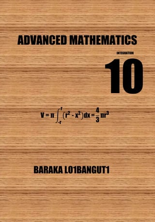
  • 1. Integration 1 | I n t e g r a t i o n ADVANCED MATHEMATICS INTEGRATION 10 BARAKA LO1BANGUT1 V = π ∫ (r2 - x2 )dx r -r = 4 3 πr3
  • 2. Integration 2 | I n t e g r a t i o n The author Name: Baraka Loibanguti Email: barakaloibanguti@gmail.com Tel: +255 621 842525 or +255 719 842525
  • 3. Integration 3 | I n t e g r a t i o n Read this! ▪ This book is not for sale. ▪ It is not permitted to reprint this book without prior written permission from the author. ▪ It is not permitted to post this book on a website or blog for the purpose of generating revenue or followers or for similar purposes. In doing so you will be violating the copyright of this book. ▪ This is the book for learners and teachers and its absolutely free.
  • 4. Integration 4 | I n t e g r a t i o n To myself and I
  • 5. Integration 5 | I n t e g r a t i o n INTEGRATION Integration is process of reversing differentiation. Previously, we learned differentiation of different relations. Here we are going to find out the relation/function whenever the derivative is given. The required relation/function is called anti – derivative or definite integrals. The origin of integral calculus can be traced back to the ancient Greeks. They were motivated by the need to measure the length of curves, the area of a surface, or the volume of a solid. Archimedes used techniques very similar to actual integration to determine the length of a segment of a curve. Democritus 410 B.C. had the insight to consider that a cone was made up of infinitely many planes cross sections parallel to the base. The theory of integration received very little stimulus after Archimedes’ remarkable achievements. It was not until the beginning of the 17th century that the interest in Archimedes’ ideas began to develop. Johann Kepler 1571 – 1630 A.D. was the first among European mathematicians to develop the ideas of infinitesimals in connection with integration. The use of the term ‘‘integral’’ is due to the Swiss mathematician Johann Bernoulli 1667 – 1748. In the present chapter, we shall study integration of real-valued functions of a single variable according to the concepts put forth by the German mathematician Georg Friedrich Riemann 1826 – 1866. He was the first to establish a rigorous analytical foundation for integration, based on the older geometric approach. Suppose we are given the function 3 4 3 2 − + = x x y , it is the derivative 4 6 + = x dx dy . The question is can do reverse to find y? It is possible to get y , the rule that guide integration is  + + = + A n x dx x n n 1 1 where A is a constant of integration and 1 −  n . So for the derivative 4 6 + = x dx dy multiply both sides dx Chapter 10 BARAKA LO1BANGUT1
  • 6. Integration 6 | I n t e g r a t i o n ( )dx x dx dy dx 4 6 + =  ( )dx x dy 4 6 + = Put the integral both sides, as ( )   + = dx x dy 4 6    + = dx xdx dy 4 3 thus   + = dx dx x y 4 3 therefore A x x y + + = 4 2 3 2 Indefinite integrals The indefinite integrals: These are integrals of the form  dx x f ) ( thus if ( )     =  dx x g dx x f dx x g x f ) ( ) ( ) ( ) ( Evaluate the integral ( )  + + dx x x 7 4 2 2 3 Solution From ( )  + + dx x x 7 4 2 2 3 ( )     + + = + + dx dx x dx x dx x x 7 4 2 7 4 2 2 3 2 3    + + dx dx x dx x 7 4 2 2 3 thus A x x x + +         +         = 7 3 4 4 2 3 4 ( )  + + + = + +  A x x x dx x x 7 3 4 2 7 4 2 3 4 2 3 Evaluate ( )  − dx x 3 2 Solution From ( )    − = − dx xdx dx x 3 3 3 2   − dx xdx 3 2 thus ( )  + − = − A x x dx x 3 3 2 2 Example 1 Example 2
  • 7. Integration 7 | I n t e g r a t i o n Evaluate        − + − dx x x x x 1 6 5 3 3 2 Solution ( )    − = − xdx dx x dx x x 5 3 5 3 2 2 thus A x x +         −         = 2 5 3 3 2 3 ( )  + − = −  A x x dx x x 2 5 5 3 2 3 2 Evaluate ( )  + − dx x x 3 5 3 2 Solution From ( )     + − = + − dx x xdx dx dx x x 3 3 5 3 2 5 3 2 A x x x +         +         − = 4 5 2 3 2 4 2 Therefore ( ) A x x x dx x x + + − = + −  4 5 2 3 2 5 3 2 4 2 3 Evaluate ( )  − dx x x 2 3 3 Solution Given ( )  − dx x x 2 3 3 thus ( )    − = − dx x dx x dx x x 2 3 2 3 3 3 Example 3 Example 4 Example 5 ( )  + − = −  A x x dx x x 3 4 2 3 4 3
  • 8. Integration 8 | I n t e g r a t i o n EXERCISE 1 1. ( )  + − dx x x 5 2 2 3 2. ( )( )  − − dx x x x 2 2 2 3 3. ( )  + − dx x x 2 5 4 3 4.        + + − dx x x x 12 5 3 3 4 3 5. ( )  − + − dx x x x 3 4 2 10 3 4 6.        + − dx x x x 2 1 3 6 1 2 3 7. ( )  − dx x x 4 3 2 8.        − dx x x 2 3 1 9. ( )  − + − dx x x x x 2 3 4 2 10.        + + dx x x x 3 1 11.        − dx x x 5 3 1 2 12.        − dx x x x 3 4 5 Substitution / Change of variable Integrals of the form  dx x f x f ) ( ' ) ( are easily evaluated by letting ) ( ' ) ( x f dx du x f u =  = hence ) ( ' x f du dx = Evaluate the integral ( )( )  − + + dx x x x 2 3 3 2 2 Solution From ( )( )  − + + dx x x x 2 3 3 2 2 Let 2 3 2 − + = x x u then 3 2 + = x dx du Make dx the subject and substitute ( ) 3 2 + = x du dx then ( ) ( )  + + 3 2 3 2 x du u x Example 6
  • 9. Integration 9 | I n t e g r a t i o n  +         = A u udu 2 2 But 2 3 2 − + = x x u ( )( ) ( )  + − + = − + + A x x dx x x x 2 2 2 2 3 2 1 2 3 3 2 Evaluate ( )( )  − − dx x x x 12 2 6 2 2 Solution From ( )( )  − − dx x x x 12 2 6 2 2 , Let x x u 12 2 2 − = and 12 4 − = x dx du ( ) 6 2 2 − = x du dx and ( ) ( )  − − 6 2 2 6 2 x du u x A u udu +         =  2 2 1 2 1 2 But x x u 12 2 2 − = ( )( ) ( )  + − = − −  A x x dx x x x 2 2 2 12 2 4 1 12 2 6 2 Evaluate ( ) ( )  + + dx x x x 5 5 1 3 3 2 Solution Let x x u x x u 5 5 5 5 3 2 3 + =  + = 5 15 2 2 + = x dx du u Substituting ( ) 1 3 5 2 2 + = x udu dx and ( ) ( )  + + 1 3 5 2 1 3 2 2 x udu u x A u du u + =  3 2 15 2 5 2 But ( ) x x u 5 5 3 + = ( ) ( )  +       + = + + A x x dx x x x 3 3 3 2 5 5 15 1 5 5 1 3 Therefore, ( ) ( ) ( ) ( )  + + + = + + A x x x x dx x x x 5 5 5 5 15 1 5 5 1 3 3 3 3 2 Example 7 Example 8
  • 10. Integration 10 | I n t e g r a t i o n Evaluate ( )( )  − + + dx x x x 5 2 1 2 7 1 7 Solution Given ( )( )  − + + dx x x x 5 2 1 2 7 1 7 Let 1 2 7 2 − + = x x u therefore ( ) 1 7 2 + = x du dx thus ( ) ( )  + + 1 7 2 1 7 5 x du u x  + = A u du u 6 5 12 1 2 1 But 1 2 7 2 − + = x x u Therefore, ( )( ) ( ) A x x dx x x x + − + = − + +  6 2 5 2 1 2 7 12 1 1 2 7 1 7 Evaluate ( )( )  − − dx x x x 9 2 4 3 3 2 Solution ( )( )  − − dx x x x 9 2 4 3 3 2 Let x x u 4 3 2 − = then 4 6 − = x dx du ( ) x du du 3 2 2 − − = then ( ) ( )  − − − x du u x 3 2 2 3 2 9 , But x x u 4 3 2 − = ( )  + − − = − A x x du u 10 2 9 4 3 20 1 2 1 ( )( ) ( ) A x x dx x x x + − − = − −  10 2 9 2 4 3 20 1 4 3 3 2 EXERCISE 2 Evaluate the following 1. ( )( )  + − − dx x x x 2 3 1 6 2 2. ( )  + − − dx x x x 3 2 3 4 4 1 2 3.  dx x x 3 cos 3 sin 4. xdx x cos sin7  5.  xdx 3 cos 6.  xdx x 3 cos 5 sin 7.  xdx x 3 sin cos 8.  xdx x 4 cos 4 sin2 Example 9 Example 10
  • 11. Integration 11 | I n t e g r a t i o n 9. ( )  + dx x x 4 2 2 3 10. ( )  + dx x 4 1 2 11.  dx x x 2 tan 12. ( )  + dx x 1 3 cos 13.  x x x d tan sec 3 14. ( )( )  − − dx x x x 5 3 2 2 1 15. dx x x  2 3 cos sin 16. dx x x  cos sin 17. dx x  5 sin 18.  xdx x 2 2 sec tan 19.  − dx x a x 2 2 20.  + dx x x 2 1 Integration of natural logarithm From, ( ) x x dx d 1 = ln ( ) dx x x d 1 = ln ( )   = dx x x d 1 ln  = dx x x 1 ln  + =  A x x dx ln thus  + = + b ax A a dx b ax ln 1 1 Integral of the form ( ) ( )  dx x f x f' Suppose you have ( ) ( )  dx x f x f' Let ( ) ( )dx x f du x f u ' =  =  + = A u u du ln But ( ) x f u = ( ) ( ) ( ) A x f dx x f x f + =  ln ' Evaluate  + 1 2x dx Example 11
  • 12. Integration 12 | I n t e g r a t i o n Solution From  + 1 2x dx Let 1 2 + = x u 2 = dx du 2 du dx =        2 1 du u thus  + = A u u du ln 2 1 2 1 , But 1 2 + = x u  + + = +  A x x dx 1 2 ln 2 1 1 2 Evaluate  + dx x x 9 3 2 Solution  + dx x x 9 3 2 Let 9 3 2 + = x u x dx du 6 = x du dx 6 = Substituting              x du u x 6  + + = A x u du 9 3 ln 6 1 6 1 2 But 9 3 2 + = x u  + + = +  A x dx x x 9 3 ln 6 1 9 3 2 2 Evaluate  − + dx x x x 1 3 2 Solution  − + dx x x x 1 3 2 simplifying            − + dx x x x x x 2 1 2 1 2 1 2 1 3 ( )    − − + dx x dx x dx x 5 . 0 5 . 0 5 . 1 3 Example 12 Example 13
  • 13. Integration 13 | I n t e g r a t i o n A x x x + + + = 2 1 2 3 2 5 2 2 2 5 A x x x dx x x x + + + =         − +  2 1 2 3 2 5 2 2 2 5 2 1 3 Evaluate  + dx x x 2 sin cos Solution From  + dx x x 2 sin cos Let 2 sin + = x u xdx du x dx du cos cos =  =  + = A u u du ln But 2 sin + = x u  + + = +  A x dx x x 2 sin ln 2 sin cos Find          + − − − dx e e e e x x x x 2 2 2 2 Solution Let x x e e u 2 2 − + = thus ( ) x x e e dx du 2 2 2 − − = ( )dx e e du x x 2 2 2 − − =   + = = A u u du u du ln 2 1 2 1 2 But x x e e u 2 2 − + =  + + =         + −  − − − A e e dx e e e e x x x x x x 2 2 2 2 2 2 ln 2 1 Example 14 Example 15
  • 14. Integration 14 | I n t e g r a t i o n Find  − + + dx x x x 2 3 3 2 2 Solution Let 2 3 2 − + = x x u then 3 2 3 2 + =  + = x du dx x dx du        + + 3 2 3 2 x du u x A u u du + =  ln , But 2 3 2 − + = x x u  + − + = − + +  A x x dx x x x 2 3 ln 2 3 3 2 2 2 Find  + − − dx x x x 7 5 3 5 3 2 Solution From  + − − dx x x x 7 10 3 5 3 2 Let 7 10 3 2 + − = x x u 10 6 − = x dx du ( ) 5 3 2 − = x du dx ( )   + = = − − A u u du x du u x ln 2 1 2 1 5 3 2 5 3 But 7 10 3 2 + − = x x u Therefore,  + + − = + − − A x x dx x x x 7 10 3 ln 2 1 7 10 3 5 3 2 2 Example 16 Example 17
  • 15. Integration 15 | I n t e g r a t i o n Evaluate  + − dx x x x 3 2 2 Solution Separate the integrals as  + − dx x x x 3 2 2 thus    + − x dx dx xdx 3 2 A x x x x x x + + − = + −  ln 3 2 2 3 2 2 2 Find  dx x x sin ln cot Solution  dx x x sin ln cot Let x u sin ln = x dx du cot = x du dx cot =        x du u x cot cot thus  + = A u u du ln but x u sin ln = A x dx x x + =  sin ln ln sin ln cot EXERCISE 3 Evaluate the following integrals. 1.        + dx x x cos 5 sin 2.  + − dx x x x x sin cos sin cos 3.        + dx x x 3 sin 1 3 cos 4.        − + + dx x x x 1 3 3 2 2 Example 18 Example 19
  • 16. Integration 16 | I n t e g r a t i o n 5.          dx x x tan 3 sec2 6.  + dx x 3 2 1 7. ( )  + dx x x 4 3 2 8 8.          + dx x x 8 3 2 9.  + dx x x sin cos 1 10.  − dx x x 3 11.  − + dx x x 3 2 12.  − + dx x x 2 4 3 2 13.  − − dx x x 2 1 3 14.  − dx x x 2 2 1 15.  − 2 2 1 x x dx 16.  −1 2 2 x x dx 17. dx x x  − 4 4 18.  + dy y y 20 9 3 Standard integrals 1. A n x dx x n n + + = +  1 1 2.  + − = A x xdx cos sin 3.  + = A x xdx sin cos 4. A x x xdx + = − =  sec ln cos ln tan 5.  + = A x xdx sin ln cot 6.  + + = A x x xdx tan sec ln sec 7.  + − = A x xdx cot cosec 8.  + = A x xdx x sec tan sec 9.  + = A x xdx tan sec2 9. A x xdx + − =  cot cosec2 10.  + = A e dx e x x 11.  + = A a a dx a x x ln , 0  a 12.  + = − − A x x dx ) ( cos 1 2 1 13.  + = + − A x x dx ) ( tan 1 2 1
  • 17. Integration 17 | I n t e g r a t i o n 14.  + = − − A x x x dx ) ( sec 1 2 1 15.  + = − − A x x dx ) ( tanh 1 2 1 16.  + = A x xdx sinh cosh 17.  + = A x xdx cosh sinh 18.  + = A x xdx cosh ln tanh 19. ( )  + = + − A x dx x 1 2 1 1 sinh 20. A x x xdx + − =  cot cosec ln cosec  dx x f ) ( sin INTEGRAL OF TRIGONOMETRIC RATIOS OF THE FORM or  dx x f ) ( cos or  dx x f ) ( tan Integrate  xdx 3 sin Solution From  xdx 3 sin Let x u 3 = , 3 du dx =        3 sin du u thus  + − = A u udu cos 3 1 sin 3 1 But x u 3 =  + − =  A x xdx 3 cos 3 1 3 sin Find ( )  + dx x x 2 tan 5 cos Solution ( )  + dx x x 2 tan 5 cos thus A x x xdx xdx + − = +   2 cos ln 2 1 5 sin 5 1 2 tan 5 cos Integrate  xdx x 5 cos 4 sin Solution Example 20 Example 21 Example 22
  • 18. Integration 18 | I n t e g r a t i o n From  xdx x 5 cos 4 sin Recall: ( ) ( ) B A B A B A sin cos 2 sin sin = − − + ( )   − = dx x x xdx x sin 9 sin 2 1 5 cos 4 sin 2 2 1 A x x xdx x + + − =  cos 2 1 9 cos 18 1 5 cos 4 sin Evaluate the integral dx x  7 cos Solution   = xdx x xdx cos cos cos 6 7 thus ( )  xdx x cos cos 3 2 ( )  − xdx x cos sin 1 3 2 Let x u sin = thus xdx du cos = substituting ( )  − du u 3 2 1 then ( )  − + − du u u u 6 4 2 3 3 1 ( ) A u u u u u + − + − = −  7 5 3 3 2 7 1 5 3 1 But x u sin = Therefore A x x x xdx + − + − =  7 5 3 7 sin 7 1 sin 5 3 sin sin cos INTEGRATION BY PART Refer product rule of differentiation ( ) dx du v dx dv u uv dx d + = Then vdu udv uv d + = ) ( Integrating both sides ( )    + = vdu udv uv d thus   + = vdu udv uv Therefore   − = vdu uv udv This is the formula of integrating by part To get the function u consider the word ILATE where, I – Inverse of trigonometric functions L – Logarithmic functions Example 23
  • 19. Integration 19 | I n t e g r a t i o n A – Algebraic functions T – Trigonometric functions (common and natural logarithm) E – Exponential functions The function that comes first is u any other function is dv. Evaluate  xdx x cos Solution Consider ILATE, therefore, Algebra comes before Trigonometric We let x u =  dx du= and xdx dv cos =   = xdx dv cos  x v sin =   − = xdx x x xdx x sin sin cos thus  + + = A x x x xdx x cos sin cos Evaluate  dx e x x 2 Solution Let 2 x u = xdx du 2 =  and   = dx e dv x x e v =    − = dx xe e x dx e x x x x 2 2 2 But  dx xex need by part integration dx e xe dx xe x x x   − = A e xe dx xe x x x + − =  thus for ( ) A e xe e x dx e x x x x x + − − =  2 2 2 Therefore, A e xe e x dx e x x x x x + + − =  2 2 2 2 Find  xdx ex cos Solution Let xdx du x u sin cos − =  = and dx e dv x = thus x x e v dx e dv =  =   Example 24 Example 25 Example 26
  • 20. Integration 20 | I n t e g r a t i o n Substituting   + = xdx e x e dx x e x x x sin cos cos dx x e x e xdx e x x x   − = cos sin sin dx x e x e x e dx x e x x x x   − + = cos sin cos cos A x e x e xdx e x x x + + =  sin cos cos 2 ( ) A x x e xdx e x x + + =  sin cos 2 1 cos Evaluate dx x x  ln 4 Solution From dx x x  ln 4 , Let dx x du x u 1 =  =ln and dx x dv 4 = 5 4 5 1 x v dx x dv =  =   thus         − = dx x x x x dx x x 1 5 1 ln 5 1 ln 5 5 4 A x x x dx x x + − =  5 5 4 25 1 ln 5 1 ln The tabular method or tic – tac – toe method So far we saw the process of evaluating integrals by using by part technique, but what will happen when you have the integral like  dx e x x 4 ? This cause a repetition of a by part method. To avoid repetition of by part process in integration, we introduce this method to simplify the repeating of the by part integration process. Suppose we want to evaluate  dx e x x 4 if we use by part method we will repeat the process 4 – times. To deal with this, we introduce the so called tabular method or tic – tac – toe method. Integrate  dx e x x 4 Solution Example 27 Example 28
  • 21. Integration 21 | I n t e g r a t i o n From  dx e x x 4 Let 4 x u = and dx e dv x = Consider the table below:- u sign dv 4 x + x e 3 4x – x e 2 12x + x e x 24 – x e 24 + x e 0 x e x e We multiply by following an arrow direction and the appropriate sign to connect each product is shown. Therefore, ( ) A e x x x x dx e x x x + + − + − =  24 24 12 4 2 3 4 4 Integrate ( )dx x  ln Solution dx x ln Let dx x du x u 1 =  =ln and x v dx dv =  =   − = dx x x dx x ln ln therefore A x x x dx x + − =  ln ln Integrate  − dx x) ( tan 1 Solution  − dx x) ( tan 1 , Let 2 1 1 x dx du x u + =  = − tan and x v dx dv =  = ( )   + − = − − 2 1 1 1 tan tan x xdx x x dx x therefore, ( ) ( )  + + − = − − A x x x dx x 2 1 1 1 ln 2 1 tan tan Example 29 Example 30
  • 22. Integration 22 | I n t e g r a t i o n EXERCISE 4 Evaluate the following integrals by using by part method 1.  xdx x sin 2.  xdx x cos 3 3.  − xdx 3 sin 1 4.  xdx x sin 4 5.  xdx ln 6.  − − dx x x x 2 1 1 sin 7.  dx e x x 3 8.  xdx 2 sin 9.  xdx x 3 sin 10.          − dx x x 2 1 sin 11. ( )  dx x e x sin 2 12.          + − − − − − dx x x x x 1 1 1 1 cos sin cos sin 13. ( )  + xdx x ln 2 2 14. ( )  + dx x x 2 1 ln 15.  + − dx x x x 2 1 2 1 tan 16.  dx e x x 3 2 17.  xdx x ln 2 18.  − xdx e x cos 19. ( )  dx x x 2 3 ln 20. ( )  − − dx x x x 2 3 2 1 2 1 sin
  • 23. Integration 23 | I n t e g r a t i o n Integration by partial fractions Case 1: When the denominator of the rational function contain linear factors, thus; ( )( ) q kx Z d cx B b ax A q kx d cx b ax x f + + + + + + = + + + + + ... ) ( ... ) ( where A, B, Z, a, b, c, d, k, q are constants. Integrate ( )( )  + − + dx x x x 1 2 2 3 Solution From ( )( )  + − + dx x x x 1 2 2 3 Decompose the rational function into small rational fractions ( )( ) 1 2 2 1 2 2 3 + + − = + − + x B x A x x x Find the values of A and B ( )( ) 1 2 2 1 2 2 3 + + − = + − + x B x A x x x By comparison; ( ) ( ) 2 1 2 3 − + + = + x B x A x When 2 = x then 1 = A and when 2 1 − = x then 1 − = B ( )( ) ( ) 1 2 1 2 1 1 2 2 3 + − − = + − + x x x x x ( )( ) ( )    + − − = + − + dx x dx x dx x x x 1 2 1 2 1 1 2 2 3 Therefore ( )( ) A x x dx x x x + + − − = + − +  1 2 ln 2 1 2 ln 1 2 2 3 Evaluate ( )( )  + + − dx x x x 1 2 1 3 4 Solution From ( )( )  + + − dx x x x 1 2 1 3 4 Example 31 Example 32
  • 24. Integration 24 | I n t e g r a t i o n Let ( )( ) 1 2 1 3 1 2 1 3 4 + + + = + + − x B x A x x x then ( ) ( ) 1 3 1 2 4 + + + = − x B x A x Compare the coefficients,    − = + = + 4 1 3 2 B A B A Solve for A and B, using a calculator, 13 − = A and 9 = B ( )( ) 1 2 9 1 3 13 1 2 1 3 4 2 + + + − = + + − x x x x x x ( )( )    + + + − = + + − dx x dx x dx x x x x 1 2 9 1 3 13 1 2 1 3 4 2 therefore ( )( )  + + + + − = + + − A x x dx x x x x 1 2 ln 2 9 1 3 ln 3 13 1 2 1 3 4 2 Solve  − + dx x x 4 3 2 Solution From  − + dx x x 4 3 2 let ( )( ) 2 2 3 4 3 2 + − + = − + x x x x x Writing into partial fractions as ( )( ) 2 2 2 2 3 + + − = + − + x B x A x x x Thus ( ) ( ) 2 2 3 − + + = + x B x A x , when 2 = x then 4 5 = A and when 2 − = x then 4 1 − = B thus, ( )( ) ( ) ( ) 2 4 1 2 4 5 2 2 3 + − − = + − + x x x x x    + − − = − + dx x dx x dx x x 2 1 4 1 2 1 4 5 4 3 2 therefore A x x dx x x + + + − = − +  2 ln 4 1 2 ln 4 5 4 3 2 Find  − − − dx x x x 2 5 3 7 2 Example 33 Example 34
  • 25. Integration 25 | I n t e g r a t i o n Solution Partialize 2 5 3 7 2 − − − x x x by factorize the denominator (if possible) ( )( ) 2 1 3 2 5 3 2 − + = − − x x x x ( )( ) 2 1 3 7 2 5 3 7 2 − + − = − − − x x x x x x ( )( ) 2 1 3 2 1 3 7 − + + = − + − x B x A x x x thus B Bx A Ax x + + − = − 3 2 7 Compare coefficients and solve for A and B    − = + − = + 7 2 1 3 B A B A 7 22 = A and 7 5 − = B thus ( )( ) ( ) ( ) 2 7 5 1 3 7 22 2 1 3 7 − − + = − + − x x x x x dx x dx x dx x x x    − − + = − − − 2 1 7 5 1 3 1 7 22 2 5 3 7 2 A x x dx x x x + − − + = − − −  2 ln 7 5 1 3 ln 21 22 2 5 3 7 2 EXERCISE 5 By partial fraction, integrate the following 1. ( )( )  + − − dx x x x 2 3 2 1 2 2. ( )( )  + + dx x x x 2 1 3. ( )( )  − − + dx x x x 2 3 2 2 4.  − 2 2 8 x dx 5. ( )( )  − + dx x x x 3 3 2 1 2 6. ( )( )  − − dx x x x sin 2 sin 1 cos 7. ( ) ( )   − = − 1 1 4 4 3 4 x x dx x x x dx 8. ( )( )( )  − + − dx x x x x 3 1 2 9. ( )( )  + − 1 1 x x x dx 10.  + dx x x 2 sin sin 1
  • 26. Integration 26 | I n t e g r a t i o n Case 2: When the denominator contain quadratic factor(s) ( )( ) ( ) q px E d cx D Cx b ax B Ax q px d cx b ax x f + + + + + + + + = + + + + + ... ... ) ( 2 2 2 2 where A, B, C, D, E, a, b, c, d, p, q are constants. Evaluate ( )( )  + − + dx x x x 2 3 2 2 Solution Partialize ( )( ) 2 3 2 3 2 2 2 + + + − = + − + x C Bx x A x x x ( ) ( )( ) 3 2 2 2 − + + + = + x C Bx x A x C Cx Bx Bx A Ax x 3 3 2 2 2 2 − + − + + = + Compare the coefficients      = + = − = + − 0 2 3 2 1 3 B A C A C B Then, 11 5 = A , 11 5 − = B and 11 4 − = C thus ( )( ) 2 3 2 3 2 2 11 4 11 5 11 5 2 + + − − = + − + x x x x x x Therefore ( )( )    + + − − = + − + dx x x dx x dx x x x 2 4 5 11 1 3 1 11 5 2 3 2 2 2 ( )( )  +         − + − = + − + − A x x x dx x x x 2 tan 11 2 2 2 3 ln 11 5 2 3 2 1 2 2 Example 35 Example 36
  • 27. Integration 27 | I n t e g r a t i o n Evaluate ( )  + + dx x x x 1 3 2 Solution Partialize ( ) 1 1 3 2 2 2 + + + = + + x C Bx x A x x x ( ) ( ) C Bx x x A x + + + = + 1 3 2 2 Cx Bx A Ax x + + + = + 2 2 2 3 then        = − = = = + 0 2 3 1 C B A B A ( )    + − = + + dx x x dx x dx x x x 1 2 3 1 3 2 2 2 ( )  + + − = + + A x x dx x x x 1 ln ln 3 1 3 2 2 2 ( )  + + = + + A x x dx x x x 1 ln 1 3 2 3 2 2 Evaluate  − + − + − dx x x x x x 9 18 2 3 4 2 3 2 Solution ( )( ) 1 2 9 3 4 9 18 2 3 4 2 2 2 3 2 − + + − = − + − + − x x x x x x x x x Partialize ( )( ) 1 2 9 1 2 9 3 4 2 2 2 − + + + = − + + − x C x B Ax x x x x ( )( ) ( ) 9 1 2 3 4 2 2 + + − + = + − x C x B Ax x x C Cx B Bx Ax Ax x x 9 2 2 3 4 2 2 2 + + − + − = + − Example 37
  • 28. Integration 28 | I n t e g r a t i o n Compare the coefficients      = + − − = + − = + 3 9 4 2 1 2 C B B A C A Then, 37 16 = A , 37 66 − = B and 37 5 = C   − + + − dx x dx x x 1 2 1 37 5 9 66 16 37 1 2    − + + − + dx x dx x dx x x 1 2 1 37 5 9 1 37 66 9 37 16 2 2 A x x x + − +       − + = − 1 2 ln 74 5 3 tan 37 22 9 ln 37 8 1 2 EXERCISE 6 Evaluate the following integrals 1. ( )( )  + + dx x x x 3 1 2 2. ( )  +1 6 x x dx 3.          − + − dx x x x x 1 2 3 4.  −1 4 x dx 5. ( )( )  − + − dx x x x 4 1 3 2 6. ( )  + dx x x 1 1 2 7. ( )( )  − + + dx x x x 2 2 5 2 8. ( )( )  − + dx x x x 1 3 1 2 9. ( )( )  − + 4 2 1 2 x x dx 10. ( )  + 2 2 x x dx
  • 29. Integration 29 | I n t e g r a t i o n Case 3: When the denominator contains the repeated root(s). ( ) ( ) ( ) ( ) ( ) q px D b ax C b ax B b ax A q px b ax x f r n n n + + + + + + + + = + + − − ... ... ) ( 1 where A, B, C, D, a, b, p, q are constants and n is a positive integer, where r is less than or equal to n. Evaluate ( )  + + dx x x x 2 2 3 1 Solution Partialize ( ) ( )2 2 2 2 3 2 3 1 + + + + = + + x C x B x A x x x ( ) ( )2 2 2 2 3 2 3 1 + + + + = + + x C x B x A x x x ( ) ( ) Cx x Bx x A x 3 2 3 2 1 2 + + + + = + When 0 = x then 4 1 = A , when 2 − = x then 6 1 = C and when 1 = x then 12 1 − = B ( ) ( )2 2 2 6 1 ) 2 ( 12 1 12 1 2 3 1 + + + − = + + x x x x x x ( ) ( )     + + + − = + + dx x dx x dx x dx x x x 2 2 2 1 6 1 2 1 12 1 1 12 1 2 3 1 Therefore, ( ) ( ) A x x x dx x x x + + − + − = + +  2 6 1 2 ln 12 1 ln 12 1 2 3 1 2 Evaluate ( )( )  − + − dx x x x 2 1 2 5 7 3 Solution Partialize ( )( ) ( )2 2 1 2 1 2 5 1 2 5 7 3 − + − + + = − + − x C x B x A x x x ( )( ) ( )2 2 1 2 1 2 5 1 2 5 7 3 − + − + + = − + − x C x B x A x x x ( ) ( )( ) ( ) 5 1 2 5 1 2 7 3 2 + + − + + − = − x C x x B x A x Example 38 Example 39
  • 30. Integration 30 | I n t e g r a t i o n      − = − = + − = − = + + = − = + − 1 when 10 4 12 9 1 when 4 6 6 0 when 7 5 5 x C B A x C B A x C B A thus 11 2 − = A , 11 4 = B and 1 − = C ( )( ) ( ) ( ) ( )2 2 1 2 1 1 2 11 4 5 11 2 1 2 5 7 3 − − − + + − = − + − x x x x x x Then ( ) ( ) ( )    − − − + + − dx x dx x dx x 2 1 2 1 1 2 1 11 4 5 1 11 2 A x x x +       − + − + + − = 1 2 1 2 1 1 2 ln 11 2 5 ln 11 2 Therefore ( )( ) A x x x x x x + − + + − = − + −  2 4 1 5 1 2 ln 11 2 1 2 5 7 3 2 EXERCISE 7 Evaluate the following integrals 1. ( )  +1 2 x x dx 2. ( )  + 2 1 x x dx 3. ( )( ) dx x x x  + + + 2 3 1 2 4. ( ) ( ) dx x x x  − + 1 2 1 3 2 5. ( )( ) dx x x x  − − + 3 1 2 3 6. ( )( ) dx x x x x  − + + + 2 2 1 3 3 2 3 7. ( )  − − dx x x 3 2 1 3 8. ( ) ( )  + − + − dx x x x x 1 5 3 1 3 2 2 2 9. ( ) ( )  + − dx x x x 2 2 1 1 4 10. ( )( )( )  − + − + dx x x x x 1 3 1 2 4 2 Case 4: When the denominator has no real factors or cannot be factorized easily k n r n n n dx cx bx ax x f − − − + + + 2 ) ( Find (a)  + + dx x x 2 2 4 2 (b)  + + 3 11 2 2 x x dx Solution Example 40
  • 31. Integration 31 | I n t e g r a t i o n (a)  + + dx x x 2 2 4 2 Consider ( ) 1 1 2 2 2 2 + + = + + x x x therefore, ( ) 1 1 4 2 2 4 2 2 + + = + + x x x ( )   + + = + + dx x dx x x 1 1 4 2 2 4 2 2 thus ( ) ( )   + + = + + dx x dx x 1 1 1 4 1 1 4 2 2 Let  tan 1 = + x Hence  d dx 2 sec = thus  + = + A d     4 1 tan sec 4 2 2 Therefore, ( )  + + = + + − A x dx x x 1 tan 4 2 2 4 1 2 (b)  + + 3 11 2 2 x x dx The expression 8 97 4 11 2 3 11 2 2 2 −       + = + + x x x therefore,   −       + = + + 8 97 4 11 2 3 11 2 2 2 x dx x x dx               + − − =       + − − 2 2 4 11 97 4 1 97 8 4 11 97 16 1 97 8 x dx x dx (See the hyperbolic substitution section) Let       + = 4 11 97 4 tanh x  then 4 11 tanh 4 97 + = x  hence dx d =   2 sech 4 97 Substituting    − = − −     d d 4 97 97 8 tanh 1 sech 4 97 97 8 2 2 C + −  97 2 replacing  , then C x +       + − − 97 11 4 tanh 97 2 1
  • 32. Integration 32 | I n t e g r a t i o n Therefore,  +       + − = + + − A x x x dx 97 11 4 tanh 97 2 3 11 2 1 2 EXERCISE 8 Evaluate the following 1.  + − 3 2 2 x x dx 2.  + + 1 7 5 2 x x dx 3.  +8 2 2 x dx 4.  + + 1 2 2 2 x x dx 5.  + − 1 2 2 x x dx 6.  + − 5 2 2 x x dx 7.  + + 11 4 2 2 x x dx 8.  + − 7 8 4 2 x x dx 9. dx x x  − + 2 3 2 2 10. dx x x  + − 2 3 3 5 2 Case 5: The use of ( ) B D dx d A N + = , where N is Numerator, D is denominator, A and B are constants, ) ( ) ( x g x f then B dx dg A x f + = ) ( Evaluate  + + − dx x x x 5 3 3 2 2 Solution From 5 3 3 2 2 + + − x x x Let ( ) B D dx d A N + = then ( ) B x A x + + = − 3 2 3 2 B A Ax x + + = − 3 2 3 2 hence 1 = A and 6 − = B 6 3 2 3 2 − + = − x x 5 3 6 3 2 5 3 3 2 2 2 + + − + = + + − x x x x x x Example 41
  • 33. Integration 33 | I n t e g r a t i o n 5 3 6 5 3 3 2 5 3 6 3 2 2 2 2 + + − + + + = + + − + x x x x x x x x    + + − + + + = + + − + dx x x x x x dx x x x 5 3 6 5 3 3 2 5 3 6 3 2 2 2 2 A x x x dx x x x +         + − + + = + + − −  11 3 2 tan 11 12 5 3 ln 5 3 3 2 1 2 2 Evaluate  + − − + dx x x x x 8 6 3 3 2 2 Solution The rational function involved in this integral is an improper rational function. So divide first to lower the numerator degree. Use long division method, 1 11 9 8 6 3 3 8 6 2 2 2 − + − − + + − x x x x x x x 8 6 11 9 1 2 + − − + x x x   + − − + dx x x x dx 8 6 11 9 2 Now Partialize, ( )( ) 4 2 11 9 8 6 11 9 2 − − − = + − − x x x x x x ( )( ) 4 2 4 2 11 9 − + − = − − − x B x A x x x ( ) ( ) 2 4 11 9 − + − = − x B x A x When 4 = x , 2 25 = B and when 2 = x , 2 7 − = A Example 42
  • 34. Integration 34 | I n t e g r a t i o n    − − − + 2 2 7 3 2 25 x dx x dx dx Therefore, ( ) ( ) A x x x dx x x x x + − − − + = + − − +  2 ln 2 7 4 ln 2 25 8 6 3 3 2 2 Evaluate  + + dx x x 5 2 2 4 Solution From  + + dx x x 2 5 2 4 Dividing by long division 2 9 4 2 5 2 2 5 0 2 2 2 2 2 4 2 4 2 − − − + − + − + + + x x x x x x x x 2 9 2 2 5 2 2 4 + + − = + + x x x x ( )    + + − = + + dx x dx x dx x x 2 9 2 2 5 2 2 2 4  +         + − = + + − A x x x dx x x 2 tan 2 9 2 3 2 5 1 3 2 4 EXERCISE 9 Evaluate the following integrals 1.  + + − dx x x x 2 3 2 1 2 2 2.  + + + dx x x x 1 4 2 Example 43
  • 35. Integration 35 | I n t e g r a t i o n 3.  + + + dx x x x 2 2 2 3 2 4.  − + + dx x x x 7 4 5 2 2 5.  + + dx x x 4 5 2 2 6.  + + dx x x 6 2 3 2 2 7. ( )  + + dx x x x 4 2 2 8.  + − + dx x x x 1 2 3 2 9.  + + − dx x x x 4 3 3 5 2 10.  − − + dx x x x 3 2 1 2 11.  + − − dx x x x 3 1 2 12.  + + − dx x x x 1 9 3 2 2 INTEGRATION OF TRIGONOMETRIC FUNCTIONS Case 6: The use of ( ) BD D dx d N + = (for trigonometric) where N is Numerator, D is denominator and A and B are constants Integrals of the form  + + dx x b c x b c x b c x b c 3 4 3 3 1 2 1 1 cos sin cos sin Evaluate dx x x x  − sin 2 cos sin Solution From dx x x x  − sin 2 cos sin Let ( ) BD D dx d N + = ( ) ( ) x x B x x dx d A x sin 2 cos sin 2 cos sin − + − = x B x B x A x A x sin 2 cos cos 2 sin sin − + − − = Compare    = + − = − − 0 2 1 2 B A B A Solve for A and B, 5 1 − = A and 5 2 − = B Example 44
  • 36. Integration 36 | I n t e g r a t i o n ( ) ( )    − − − − + = − dx x x x x dx x x x x dx x x x sin 2 cos sin 2 cos 5 2 sin 2 cos cos 2 sin 5 1 sin 2 cos sin Consider  − + dx x x x x sin 2 cos cos 2 sin 5 1 , Let x x u sin 2 cos − = ( )dx x x du cos 2 sin + − =  − = u u du ln 5 1 5 1 , But x x u sin 2 cos − = x x dx x x x x sin 2 cos ln 5 1 sin 2 cos cos 2 sin 5 1 − − = − +  Also consider x dx dx x x x x 5 2 5 2 sin 2 cos sin 2 cos 5 2 − = − = − −   Therefore, A x x x dx x x x + − − − = −  5 2 sin 2 cos ln 5 1 sin 2 cos sin Evaluate dx x x x  + sin cos 3 cos Solution From dx x x x  + sin cos 3 cos ( ) ( ) x x B x x dx d A x sin cos 3 sin cos 3 cos + + + = x B x B x A x A x sin cos 3 sin 3 cos cos + + − = Compare coefficients    = + − = + 0 3 1 3 B A B A Solve for A and B then 10 1 = A and 10 3 = B    + + + + − = + dx x x x x dx x x x x dx x x x sin cos 3 sin cos 3 10 3 sin cos 3 sin 3 cos 10 1 sin cos 3 cos  + + + = + A x x x dx x x x 10 3 sin cos 3 ln 10 1 sin cos 3 cos Example 45
  • 37. Integration 37 | I n t e g r a t i o n EXERCISE 10 Evaluate the following integrals 1.  + dx x x x 2 sin 2 cos 2 sin 2.  − + dx x x x x cos 5 sin 7 cos sin 2 3.  + + dx x x x x cos 4 sin 3 cos 3 sin 2 4.  + dx x x x cos 4 sin 3 cos 3 5.  dx x x cos sin 5 6. dx x x  + 5 cos 2 sin 4 7.  + dx x x x sin cos sin 8.  + dx x x x sin 4 cos cos 3 9.  + − dx x x x x sin cos sin cos 10.  dx x x cos tan Integrals of the form (a)  + x b a dx cos (b)  + x b a dx sin (c)  + x b x a dx sin cos Use of t formula Refer, 2 2 1 1 cos t t x + − = and 2 1 2 sin t t x + = where       = 2 tan x t Solve  + x dx cos 5 3 Solution  + x dx cos 5 3 Let       = 2 tan x t then       = 2 sec 2 1 2 x dx dt Thus dx x dt =       2 sec 2 2 Example 46
  • 38. Integration 38 | I n t e g r a t i o n But 2 2 1 1 cos t t x + − =          + − + + 2 2 2 1 1 5 3 1 2 t t t dt then ( ) ( )   − = − + + 2 2 2 2 8 2 1 5 1 3 2 t dt t t dt ( )   − = − 2 2 2 1 4 1 4 t dt t dt , Let  tanh 2 = t thus  d dt 2 sech 2 =  + = − A d se     2 1 tanh 1 ch 2 4 1 2 2 But       = − 2 tanh 1 t  and       = 2 tan x t A x x dx +               = + −  2 tan 2 1 tanh cos 5 3 1 Solve  − x dx cos 3 5 Solution From  − x dx cos 3 5 Let       = 2 tan x t then       = 2 sec 2 2 x dt dx therefore 2 1 2 t dt dx + =   + =         + − − + 2 2 2 2 8 2 2 1 1 3 5 1 2 t dt t t t dt thus ( )   + = + 2 2 2 1 8 2 2 t dt t dt Example 47
  • 39. Integration 39 | I n t e g r a t i o n    d dt t 2 sec 2 1 tan 2 =  = therefore ( )   + = + = + A d t dt     2 1 tan 1 sec 2 1 2 1 2 2 2 But ( ) t 2 tan 1 − =  and       = 2 tan x t thus A x x dx +               = − −  2 tan 2 tan 2 1 cos 3 5 1 Integrate  + x dx sin 1 Solution From  + x dx sin 1 , Let       = 2 tan x t then       = 2 sec 2 1 2 x dx dt thus 2 2 1 2 2 sec 2 t dt x dt dx + =       = substituting   + + = + + + dt t t dt t t t 2 2 2 2 1 2 1 2 1 1 2 ( ) dt t dt t t   + = + + 2 2 1 2 2 1 2 Let 1 + = t u then dt du=  + − = A u u du 2 2 2 but 1 + = t u ( )  + + − = + A t t dt 1 2 1 2 2 but       = 2 tan x t  + +       − = + A x x dx 1 2 tan 2 sin 1 Evaluate  +6 sin 4 cos 3 x x dx Solution Example 48 Example 49
  • 40. Integration 40 | I n t e g r a t i o n From  +6 sin 4 cos 3 x x dx , Let dx x dt x t       =        = 2 sec 2 1 2 tan 2 then  +       + +         + −       + 6 1 2 4 1 1 3 2 tan 1 2 2 2 2 2 t t t t x dt  + + + + − + 2 2 2 2 1 6 6 8 3 3 1 2 t t t t t dt  + + 9 8 3 2 2 t t dt  + + 3 3 8 3 2 2 t t dt  +       + 9 11 3 4 3 2 2 t dt A t +         + − 11 4 3 tan 11 2 1 But       = 2 tan x t ( ) A x +         + − 11 4 tan 3 tan 11 2 2 1 Evaluate ( )  + 2 cos sin 2 x x dx Solution From ( )  + 2 cos sin 2 x x dx Divide by x cos ( )  + 2 1 tan 2 sec x xdx thus, ( ) 1 tan 2 2 1 + − x Example 50
  • 41. Integration 41 | I n t e g r a t i o n EXERCISE 11 Evaluate the following 1.  + − 5 sin 4 cos 3 x x dx 2.  + x dx sin 5 4 3.  − x x dx cos sin 1 4.  + − 13 sin 5 cos 12 x x dx 5.  + + 3 cos sin 2 x x dx 6.  + x dx tan 3 2 7.  + dx x x x sin 3 cos 2 sin 8.  + + dx x x x x cos sin 2 cos sin 9.  + + dx x x x sin cos 1 cos 10.  + dx x 2 sin 2 1 R– FORMULA IN INTEGRATION ( )       sin sin cos cos cos r r r  =  or ( )       sin cos cos sin sin r r r  =  Evaluate  + x x dx sin 4 cos 3 Solution  + x x dx sin 4 cos 3 Let ( )  + = + x r x x sin sin 4 cos 3   sin cos cos sin sin 4 cos 3 x r x r x x + = + x x r cos 3 sin cos =  3 sin =  r (1) x x r sin 4 cos sin =  4 cos =  r (2) Divide equation (1) by equation (2)       = − 4 3 tan 1  Square equation (1) and (2) and sum then 5 4 3 2 2 = + = r Example 51
  • 42. Integration 42 | I n t e g r a t i o n               + = + − 4 3 tan sin 5 sin 4 cos 3 1 x x x                + − 4 3 tan sin 5 1 x dx                + − dx x 4 3 tan cosec 5 1 1 A x x +               + −               + − − 4 3 tan cot 4 3 tan cosec ln 5 1 1 1 EXERCISE 12 Evaluate the following 1.  − x x dx sin 12 cos 5 2.  + x x dx sin cos 3.  + x x dx sin 7 cos 24 4. ( )  − x x dx cos sin 2 5.  + 3 tan sec2 x xdx 6.  + dx x x 4 cot cos 7.  − + dx x x x x sin cos cos 2 sin 8.  + dx x sin 3 4 9.  + dx x x 2 cos 3 2 sin 1 10.  + dx x x 4 tan sec Integral of the form  xdx x n m sin cos Evaluate  xdx 2 sin Solution Example 52
  • 43. Integration 43 | I n t e g r a t i o n Given  xdx 2 sin from x x x 2 2 sin cos 2 cos − = thus ( ) x x 2 cos 1 2 1 sin2 − = ( )   − = dx x dx x 2 cos 1 2 1 sin2 therefore A x xdx + − =  2 sin 4 1 2 1 sin2 Integrate dx x x  sin cos3 Solution Let x du dx x u sin cos − =  = A u du u x du x u + − = − = −   4 3 3 4 1 sin sin But x u cos = then A x xdx x + − =  4 3 cos 4 1 sin cos Evaluate dx x x  2 3 sin cos Solution   = xdx x x dx x x 2 2 2 3 sin cos cos sin cos ( )   − = xdx x x xdx x x 2 2 2 2 sin sin 1 cos sin cos cos Let xdx du x u cos sin =  = ( ) A u u du u u + − = −  5 3 2 2 5 1 3 1 1 But x u sin = A x x dx x x + − =  5 3 2 3 sin 5 1 sin 3 1 sin cos Example 53 Example 54
  • 44. Integration 44 | I n t e g r a t i o n EXERCISE 13 Evaluate the following integrals 1. dx x x  2 5 cos sin 2. dx x x  4 3 cos sin 3. dx x  7 sin 4. xdx x 5 8 cos sin  5. Show that  + + + = A x x x x xdx tan sec ln 2 1 tan sec 2 1 sec3 6.  xdx x 7 5 sin cos 7.  xdx 11 cos 8. dx x x  tan sec4 9.  xdx x 2 7 sin cos 10. Show that 4 1 16 π sin 2 0 2 2 π + =  dx x x 11.  xdx x 7 3 cos sin 12.  xdx 4 cos Integrals of the form  + dx x b x a 2 2 sin cos 1 Integrate  + x x dx 2 2 sin 5 cos 3 Solution From  + x x dx 2 2 sin 5 cos 3 Divide throughout by x 2 cos  + dx x x 2 2 tan 5 3 sec Let x u tan = xdx du 2 sec =    + = + 2 2 3 5 1 3 1 5 3 u du u du Let  tan 3 5 = u  d du 2 sec 3 5 = therefore  d du 2 sec 5 3 = Example 55
  • 45. Integration 45 | I n t e g r a t i o n   = + =     d d 5 3 3 tan 1 sec 5 3 3 1 2 2 But         = − u 3 5 tan 1  A u +         − 3 5 5 3 3 1 tan But x u tan = A x +         − tan 3 15 tan 15 15 1 Therefore, A x x x dx +         = + −  tan 3 15 tan 15 15 sin 5 cos 3 1 2 2 Solve  − x dx 2 cos 1 Solution From  − x dx 2 cos 1 x x x 2 2 sin cos 2 cos − =    = = xdx x dx x dx 2 2 2 cosec 2 1 sin 2 1 sin 2 A x xdx x dx + − = = −   2 2 2 cot 2 1 cosec 2 1 cos 1  + − = − A x x dx 2 2 cot 2 1 cos 1 Evaluate  + dx x x 2 sin 4 cos Solution From  + dx x x 2 sin 4 cos Let x u sin = thus xdx du cos = Example 56 Example 57
  • 46. Integration 46 | I n t e g r a t i o n         + = + 2 2 2 1 4 1 4 u du u du A x u u du +       =       = + − −  sin 2 1 tan 2 1 2 tan 2 1 4 1 1 2 Therefore,  +       = + − A x dx x x sin 2 1 tan 2 1 sin 4 cos 1 2 Evaluate  + dx x x 2 cos 1 sin Solution From  + dx x x 2 cos 1 sin   + = + dx x x x dx x x x 2 2 2 tan 2 tan sec sin cos 2 sin  + dx x x x 2 sec 1 tan sec Let x u sec = xdx x du tan sec =  ( )  + = + − A u u du 1 2 tan 1 But x u sec = ( ) A x dx x x + = + −  sec tan cos 1 sin 1 2 Example 58
  • 47. Integration 47 | I n t e g r a t i o n EXERCISE 14 Evaluate the following 1.  + x x dx 2 2 sin 4 cos 2.  +3 2 cos x dx 3. dx x x  + 2 2 sin cos 9 1 4. dx x x  + sin cos 2 1 5. dx x x  − cos 3 sin 1 2 6.  − dx x x x sin cos sin 7.  + dx x x x cos sin 1 tan 8.  + dx x 2 cos 2 1 9.  − dx x x sec cos 4 2 10.  − + dx x x x x sin cos sin cos Integrals of the form ( ) dx r qx px b ax  + + + 2 Use ( ) B r qx px dx d A b ax + + + = + 2 if substitution technique is not working. Evaluate ( )  + + + dx x x x 1 2 2 2 2 Solution Let ( ) B x x dx d A x + + + = + 1 2 2 2 2 ( ) B x A x + + = + 2 4 2    = = + 1 4 2 2 A B A then 4 1 = A and 2 3 = B thus ( ) 2 3 2 4 4 1 2 + + = + x x ( )   + + + + + + dx x x dx x x x 1 2 2 2 3 1 2 2 2 4 4 1 2 2 Consider ( )  + + + dx x x x 1 2 2 2 4 4 1 2 , Let 1 2 2 2 + + = x x u  ( )dx x udu 2 4 2 + = thus  du u2 4 2         = 3 2 1 3 u Example 59
  • 48. Integration 48 | I n t e g r a t i o n But 1 2 2 2 + + = x x u thus 3 2 1 2 2 6 1       + + x x Consider ( )  + + dx x x 1 2 2 3 2        +       + dx x 2 2 2 1 2 1 2 2 3 dx x          +       +        1 2 1 2 2 1 2 2 3 2 dx x          +       + 1 2 1 2 4 2 3 2 , let 1 2 2 1 2 sinh + =       + = x x  thus   d dx 2 cosh =     d cosh sinh 8 2 3 2   d 2 cosh 8 2 3 thus ( )  +   d 1 2 cosh 16 2 3 A + +   16 2 3 2 sinh 32 2 3 But ( ) 1 2 sinh 1 + = − x  ( ) ( ) ( ) A x x + + + + − − 1 2 sinh 16 2 3 1 2 sinh 2 sinh 32 2 3 1 1 Combining the two solutions ( )  + + + dx x x x 1 2 2 1 2 2 ( ) ( ) ( ) A x x x x + + + + +       + + = − − 1 2 sinh 16 2 3 1 2 sinh 2 sinh 32 2 3 1 2 2 6 1 1 1 3 2 Evaluate  + − + dx x x x 1 1 2 4 2 Solution From  + − + dx x x x 1 1 2 4 2 Divide throughout by 2 x Example 60
  • 49. Integration 49 | I n t e g r a t i o n        + −       + dx x x x x x 2 2 2 2 2 1 1 1 1 complete the square              + − + − + dx x x x 2 2 1 1 1 1 2 2 2  +       − + + dx x x x 1 2 1 1 1 2 2 2 thus  +       − + dx x x x 1 1 1 1 2 2 and let dx x du x x u       + =  − = 2 1 1 1 ( ) A u u du + = + −  1 2 tan 1 but x x u 1 − = Therefore  +       − = + − + − A x x dx x x x 1 tan 1 1 1 2 4 2 EXERCISE 15 Evaluate the following integrals 1. ( )  − + dx x x 5 2 3 2 2. ( )  + + + dx x x x 1 1 2 3. ( ) ( )  − + + dx x x x 5 2 10 2 2 1 2 4.  − + − dx x x x 1 1 2 4 2 5. ( )  + + − dx x x x 8 4 2 5 2 6. ( )  + − − dx x x x 2 1 3 2 7. ( )  + − − dx x x x 3 5 2 5 7 2 8. ( )( )  − + − dx x x x 3 2 1 3 1 2 9. ( )( )  − − dx x x x 3 2 3 2 3 4 10.  − + dx x x 2 2 1 2 11.  + + − dx x x x 4 2 2 4 2 12. ( ) ( ) ( )  + + + = + + A x x dx x x 7 3 3 15 2 4 3 2 3
  • 50. Integration 50 | I n t e g r a t i o n SUBSTITUTION OF INVERSE OF TRIGONOMETRIC FUNCTIONS Integrals of the form dx x f  − 2 ) ( 1 1 or ( )  + dx x f 2 ) ( 1 1 Refer the derivatives of inverse of trigonometric functions 1. If ) ( sin 1 x y − = then 2 1 1 x dx dy − = 2. If ) ( cos 1 x y − = then 2 1 1 x dx dy − − = 3. If ) ( tan 1 x y − = then 2 1 1 x dx dy + = 4. If ) ( sec 1 x y − = then 1 1 2 − = x x dx dy 5. If ) ( csc 1 x y − = then 1 1 2 − − = x x dx dy 6. If ) ( cot 1 x y − = then 2 1 1 x dx dy + − = Evaluate dx x  − 2 9 4 1 Solution This integral resembles, cosine or sine inverse, any of the function can be used. Given dx x  − 2 9 4 1 , this can expressed as ( ) ( )   − = − dx x dx x 2 2 3 2 4 9 1 1 2 1 1 4 1 let x 2 3 sin =  , then dx d =   cos 3 2   + = = −  A d d      3 1 3 1 sin 1 cos 3 2 2 1 2 , but       = − x 2 3 sin 1  therefore A x x dx +       = −  − 2 3 sin 3 1 9 4 1 2 Example 61
  • 51. Integration 51 | I n t e g r a t i o n EXERCISE 16 Evaluate the following 1.  − 2 3 5 x dx 2.  − + dx x x 2 9 2 1 1 3.  + dx x2 49 4 1 4.  − + dx x x 2 6 1 5.  − − dx x x x 4 2 1 1 sin 6.  − + 2 3 3 x x dx 7.  + + dx x x 2 1 1 8. ( )  − − 2 1 2 4 2 x x dx 9.  − − dx e e e x x x 2 4 5 10.  − + dx x x 2 4 3 2 SUBSTITUTION OF INVERSE OF HYPERBOLIC FUNCTIONS Refer the derivatives of inverse of hyperbolic functions, for further studies of these integrals of these form, check the hyperbolic functions topic in book 2. 1. If ) ( cosh 1 x y − = then 1 1 2 − = x dx dy 2. If ) ( sinh 1 x y − = then 2 1 1 x dx dy + = 3. If ) ( tanh 1 x y − = then 2 1 1 x dx dy − = 4. If ) ( sech 1 x y − = then 2 1 1 x x dx dy − = 5. If ) ( cosech y -1 x = then 1 1 2 + = x x dx dy 6. If ) ( coth 1 x y − = then 1 1 2 − = x dx dy
  • 52. Integration 52 | I n t e g r a t i o n Integrate dx x x  − + 2 3 1 1 6 Solution From dx x x  − + 1 3 1 6 2 , thus   − + − 1 3 1 3 6 2 2 x dx dx x x INTEGRAL OF EXPONENTIAL AND LOGARITHMIC FUNCTIONS Suppose we have  dx ax , for all 0  a Let x a y = then a x y a y x ln ln ln ln =  = a dx dy y ln 1 = thus   =  = adx y dy adx y dy ln ln dx y a y  =ln but x a y = thus dx a a a x x  =ln Therefore A a a dx a x x + =  ln , where 0  a Integrate dx x x        2 3 ) ( Solution From dx x x        2 3 ) ( , let x dx dy x y 2 2 =  = ( )   = dy x dy x y y 3 2 1 2 3 , let 3 ln 2 1 = dx dy y thus   =  = ydx dy ydx dy 3 ln 2 1 3 ln 2 replacing y Therefore, A dx x x + =  9 ln 3 3 2 2 Example 63 Example 62
  • 53. Integration 53 | I n t e g r a t i o n Integrate ( )  + dx e x x 2 3 Solution ( )    + = + dx dx e dx e x x x x 2 3 2 3 thus ( ) A e dx e x x x x + + = +  2 ln 2 3 2 3 Integrate  − dx x 1 2 4 Solution Let ( ) 4 ln 1 2 ln 4 1 2 − =  = − x y y x dx y dy dx dy y 16 ln 4 ln 2 1 =  =    =  = ydx y ydx dy 16 ln 16 ln but 1 2 4 − = x y  − − = dx x x 1 2 1 2 4 16 ln 4 therefore A dx x x + = − −  16 ln 4 4 1 2 1 2 Integrate ( )  − + dx e x x x 2 3 10 Solution Using a general observation ( )  − + dx e x x x 2 3 10 Can be expressed as    − + dx e dx dx x x x 2 3 10 thus ( ) A e dx e x x x x x x + − + = − +  2 2 2 1 3 ln 3 10 ln 10 3 10 Example 64 Example 65 Example 66 Question Show that A dx x x + =  + + 9 ln 3 3 2 2 2 2
  • 54. Integration 54 | I n t e g r a t i o n Integrate  + + dx x x x x 5 2 5 ln 5 10 5 4 Solution From  + + dx x x x x 5 2 5 ln 5 10 5 4 , let x x u 5 2 5 + = thus 5 ln 5 10 4 x x dx du + = A u du u + =  ln 1 thus ( ) A x dx x x x x x + + = + +  5 2 ln 5 2 5 ln 5 10 5 5 4 DEFINITE INTEGRALS The fundamental theorem of calculus The integrals of the form ( ) ( ) ( ) a F b F dx x f b a − =  are called definite integrals. If b a = then  = − = − = b a a F a F b F b F dx x f 0 ) ( ) ( ) ( ) ( ) ( Evaluate the value of ( )  − + 2 1 3 3 2 dx x x Solution From ( ) 2 1 2 4 2 1 3 3 4 3 2 A x x x dx x x + − + = − +          +  − + −         +  − + = + − + A A A x x x 1 3 1 1 1 2 3 2 4 2 3 4 2 2 2 4 2 1 2 4 Therefore ( ) 5 3 2 2 1 3 = − +  dx x x By first expressing 3 5 2 17 4 4 2 2 − + − + x x x x into partial fractions, show that        − = − + − + 2 1 2 2 4 45 ln 2 3 5 2 17 4 4 dx x x x x Example 68 Example 69 Example 67
  • 55. Integration 55 | I n t e g r a t i o n Solution Use long division method first to simplify the function 3 5 2 17 4 4 2 2 − + − + x x x x 2 11 6 6 10 4 17 4 4 3 5 2 2 2 2 − − − + − − + − + x x x x x x x 3 5 2 11 6 2 3 5 2 17 4 4 2 2 2 − + + − = − + − + x x x x x x x Partial fractions ( )( ) 3 1 2 11 6 3 5 2 11 2 + − + = − + x x x x x ( )( ) 3 1 2 3 1 2 11 6 + + − = + − + x B x A x x x thus ( ) ( ) 1 2 3 11 6 − + + = + x B x A x When 3 − = x , 1 = B and when 2 1 = x , 4 = A ( )( ) ( ) ( ) 3 1 1 2 4 3 1 2 11 + + − = + − x x x x Now combine the solutions  − + − + 2 1 2 2 3 5 2 17 4 4 dx x x x x    + + − − 2 1 2 1 2 1 3 1 1 2 1 4 2 dx x dx x dx        − = 4 5 9 ln 2 Therefore       − = − + − +  4 45 ln 2 3 5 2 17 4 4 2 1 2 2 dx x x x x Hence shown Evaluate ( )  + 3 π tan sec 0 dx x x Solution From ( )  + 3 π 0 tan sec dx x x thus   + 3 π 3 π tan sec 0 0 xdx xdx Example 70
  • 56. Integration 56 | I n t e g r a t i o n 3 π sec ln tan sec ln 0 x x x + + = 2 3 1 ln 2 ln 3 2 ln + = + + = Therefore ( ) 2 3 1 ln tan sec 3 0 + = +   dx x x Express ( )2 3 1 2 − + x x in to partial fractions and hence show that ( ) 49 ln 6 3 1 2 10 4 2 + = − +  dx x x Solution From ( ) ( )2 2 3 3 3 1 2 − + − = − + x B x A x x and B A Ax x + − = + 3 1 2 Compare the coefficients 2 = A and 7 = B ( ) ( )2 2 3 7 3 2 3 1 2 − + − = − + x x x x ( ) ( )    − + − = − + 10 4 2 10 4 10 4 2 3 7 3 2 3 1 2 dx x dx x dx x x ( ) 10 4 10 4 2 3 7 3 ln 2 3 1 2 − − − = − +  x x dx x x ( ) ( ) ( ) 7 1 ln 2 1 7 ln 2 3 1 2 10 4 2 − − − = − +  dx x x ( ) 49 ln 6 3 1 2 10 4 2 + = − +  dx x x Hence shown Show that 4 π tan 1 2 π 0 = +  x dx Solution Example 71 Example 72
  • 57. Integration 57 | I n t e g r a t i o n Let  + = 2 π 0 tan 1 x dx In  + = 2 π 0 sin cos cos x x xdx In   + =       − +       −       − = 2 π 0 2 π 0 sin cos sin 2 sin 2 cos 2 cos x x xdx x x dx x In     + = 2 π 0 sin cos sin x x xdx In dx x x x dx x x x In   + + + = 2 π 0 2 π 0 sin cos cos cos sin sin 2  + + = 2 π 0 sin cos cos sin 2 dx x x x x In 2 π 0 2 x In = then 2 π 2 = n I therefore 4 π = n I , proved EXERCISE 17 Evaluate the following 1.        + + 8 1 3 4 3 dx x x 2. ( )( )  − + + 2 1 4 2 10 2 2 1 2 dx x x x 3.  − + + 5 1 2 5 12 3 2 dx x x x 4. ( ) − 2 π 2 π 2 sin dx x 5. ( )  + 4 1 2 3 1 dx x 6. ( )( )  + + + 2 1 3 2 1 dx x x x 7. ( )dx x x  3 π 0 cos 3 cos 8.        + 7 3 7 1 2 49 1 1 dx x 9. ( )  −       − 2 tan 4 π 1 2 sin 3 2 cos 4 3 dx x x 10. ( )dx x x  1 . 1 0 3 tan sec 11.        3 2 ln dx x x
  • 58. Integration 58 | I n t e g r a t i o n APPLICATIONS OF INTEGRATION There are several applications of integration. AREA UNDER THE CURVE:  = b a ydx Area Suppose we want to find the area under the curve ) (x f y = sketched below bounded from a x = to b x = with the curve. One way to estimate the area, A, (Figure 10.1) is to divide the area into rectangular strips, (Figure 10.2) the sum of the areas of strips is approximated to the area under the curve. The thinner the strips the better approximation, i.e. as the number of strips increase the better approximation of the area under the curve. Since each strip have the same width, δx the length of each strip is y, therefore, the area of one strip is given as x y A    , to get the area under the curve we sum the area of all strips from a x = to b x = , this can be written as  = = b a x A  Area , as the width of strips decrease, the number of rectangles increase, therefore, as 0 → x  , dx dA x A y x A x =       →  →      0 lim Then y dx dA = becomes  =  = ydx A ydx dA , the boundary limit of x is a x = to b x = . This defines the area under the curve as,  = b a ydx A . Procedures to find the area (a) Draw a sketch of the given region to visualize the nature of the curve and divide intervals appropriately to avoid getting negative or zero answer. (b) Write the defined integral(s) to represent the region A Figure 10.1 Figure 10.2 a a b b
  • 59. Integration 59 | I n t e g r a t i o n (c) Evaluate the defined integral. Determine the area under the curve 3 + − = x y from 0 = x to 2 = x Solution Sketch ( )  + − = 2 0 3 dx x A 2 0 2 3 2         + − = x x A thus 4 = A The area is four sq. units Find the area under the curve 4 2 + − = x y from 1 = x to 2 = x Solution  = b a ydx Area therefore ( )  + − = 2 1 2 4 dx x A 2 1 3 4 3 x x A + − =       + − −       + − = 4 3 1 8 3 8 A The area is 3 5 square units. Evaluate the area of the curve 2 3 2x x y + = from 1 − = x to 1 = x Solution ( ) − + = 1 1 2 3 2 dx x x A Example 70 Example 71 Example 72 4 2 + − = x y 3 + − = x y
  • 60. Integration 60 | I n t e g r a t i o n ( ) ( )   + + + = − 1 0 2 3 0 1 2 3 2 2 dx x x dx x x A 1 0 3 4 0 1 3 4 3 2 4 3 2 4         + +         + = − x x x x A 3 . 1 3 2 4 1 3 2 4 1 =       + +       − − = A The area is 1.3 square units. Determine the area of the curve 3 3 2 3 + − − = x x x y from 1 − = x to 3 = x Solution From the sketch, a part of the integral lies below the x – axis and the other part lie above, if we evaluate the integral direct from 1 − = x to 3 = x , the result will be zero, we divide the integral as follows ( ) ( )   − + − − + + − − = 0 1 2 3 3 0 2 3 3 3 3 3 dx x x x dx x x x A While dividing it, we should make sure the area obtained is always positive, this can be done by taking the absolute value of each integral above. 0 1 2 3 4 3 0 2 3 4 3 2 4 3 2 4 −         + − − +         + − − = x x x x x x x x A The area is 4.5 square units. Example 73 3 3 2 3 + − − = x x x y 2 3 2x x y + =
  • 61. Integration 61 | I n t e g r a t i o n Find the area of the curve x y sin 3 = from 0 = x to 2π = x Solution  = b a ydx A then ( )  = 2π 0 sin 3 dx x A ( ) ( )   + = 2π π π 0 sin 3 sin 3 dx x dx x A ( ) ( ) π 2 π π 0 cos 3 cos 3 x x A + = π cos 3 π 2 cos 3 0 cos 3 π cos 3 − + − = A A = 12 Square units. Find an approximate area of the shaded region below Solution ) sin( 3 x y = Example 74 2 4 x x y − = Example 75
  • 62. Integration 62 | I n t e g r a t i o n ( )  − = 4 0 2 4 dx x x A thus 4 0 3 2 3 2 x x A − = The area is 3 32 = A square units. ( )  − = b a dx y y A 2 1 AREA BETWEEN CURVES: (where a and b are abscissa at a point of intersection) If the area under the curve ) (x f y = is given by  = b a dx x f A ) ( 1 and the area under the curve ) (x g y = is given as Figure 10.3 a b ) (x f y = ) (x g y = A
  • 63. Integration 63 | I n t e g r a t i o n  = b a dx x g A ) ( 2 , then the area between the curves ) (x f y = and ) (x g y = from a x = to b x = (Where a and b are the values of x at the point of intersection of the curves) is given by    − = b a dx x g x f A ) ( ) ( , (Figure 10.3) Find the area between curves 2 4 x y − = and x x y 2 2 − = Solution First, find the points of intersection of the curves, 2 2 4 2 x x x − = − 0 4 2 2 2 = − − x x ( )( ) 0 2 1 = − + x x 1 − = x and 2 = x ( )  − = b a dx y y A 1 2 ( ) ( ) ( ) − − − − = 2 1 2 2 2 4 dx x x x A ( ) − + − = 2 1 2 2 2 4 dx x x A x x y 2 2 − = 2 4 x y − = Example 76
  • 64. Integration 64 | I n t e g r a t i o n 2 1 2 3 3 2 4 − + − = x x x A therefore the area is 9 square units Find the area enclosed by the curves 3 7 2 2 + + = x x y and 2 4 9 x x y − + = Solution The points of intersection of the curve ( )( ) 0 2 1 4 9 3 7 2 2 2 = + −  − + = + + x x x x x x thus 1 = x or 2 − = x ( )  − = b a dx y y A 1 2 ( ) ( ) ( ) − − + − + + = 1 2 2 2 4 9 3 7 2 dx x x x x A ( ) − − + = 1 2 2 6 3 3 dx x x A 1 2 2 3 6 2 3 − − + = x x x A 2 27 = A square units Find the area between curves 1 2 − = x y and x y − =1 Solution Point of intersections 1 1 2 − = + − x x 2 − = x and 1 = x ( )  − = b a dx y y A 1 2 ( ) ( ) ( ) − + − − = 2 1 2 1 1 dx x x A ( ) − − − = 2 1 2 2 dx x x A Example 77 2 4 9 x x y − + = 3 7 2 2 + + = x x y Example 78 1 2 − = x y x y − =1
  • 65. Integration 65 | I n t e g r a t i o n 2 1 2 3 2 2 3 − − − = x x x A Area is 4.5 square units Find the area of the curve x x x x y 6 3 6 3 2 3 4 + − − = with x – axis Solution The points of intersection x x x x y 6 3 6 3 2 3 4 + − − = ( )( )( ) 0 1 1 3 3 = + − − x x x x 0 = x , 3 = x , 1 = x and 1 − = x ( ) − + − − = 3 1 2 3 4 6 3 6 3 dx x x x x A 3 1 2 3 4 5 3 2 3 5 3 − + − − = x x x x A 5 2 22 = A sq. units Example 79 x x x x y 6 3 6 3 2 3 4 + − − =
  • 66. Integration 66 | I n t e g r a t i o n EXERCISE 18 1. Find the under the curve x x x f 4 ) ( 3 − = from 2 − = x to 2 = x . 2. Find the area enclosed by the x – axis and that part of the curve 2 3 2 ) ( x x x f + − = . 3. Sketch the graph of ( ) 2 ln x x y + = and hence calculate the area bounded with the x axis from 1 = x to 2 = x . 4. Find the area of the region bounded by the curve 1 2 3 2 + − = x x y , the line 0 1 = + x , 0 2 = − x and 0 = y 5. The area between the curve 9 3 2 2 = + y x and the y-axis from 3 − = y and 3 = y is rotated about the y-axis. Find the volume of the solid generated. 6. Find the area between the curve 1 + = x y and 2 3 x y − = 7. Find the area between the curves 2 y x = and 4 3 + = y x 8. Find the area bounded by the curve x y + =1 and 1 − = x y 9. Find the area between the coordinates axes and the curve 2 − = x y 10. Find the area under the curve 4 = y between the lines 0 = x and 5 = x 11. Find the area under the curve 3 1 = + x y from 0 = x to 40 = x 12. Find the area between curves 2 x y = and 2 2 + − = x y 13. Find the value of a if the area between the curve 2 2 + =ax y and 2 x y = from 1 = x to 2 = x is 10 square units. 14. Find the area between the curves x y 4 2 = and x y x 8 2 2 = + bounded with the x – axis. 15. Find the area under the curve 5 3 2 = + y y x from 0 = x to 3 = x
  • 67. Integration 67 | I n t e g r a t i o n VOLUME OF THE SOLID OF REVOLUTION Suppose the area enclosed by the line ax y = with x – axis and the line c x = is rotated through one revolution, the solid formed is called solid of revolution, which is cone in this case. Consider the figure below Volume of disc A, h πr V 2 = To get the volume of the figure from a x = to b x = is the summation of the approximated volume of the discs, given y r = and δx h = therefore volume,  = = = b x a x 2 δx πy V .   =         = = = → b a 2 b x a x 2 0 δx dx π δx π lim V y y Therefore the volume is given by  = b a dx y V 2 π A y δx b a Rotation
  • 68. Integration 68 | I n t e g r a t i o n The volume is given by  = b a dx y V 2 π , if the curve is revolved about x – axis or dy x V b a  = 2 π if the curve is revolved about y – axis. Note that, if the curve is symmetrical about the y – axis or x – axis and the same curve is made to revolve about the x – axis or y – axis, we revolve only the part of the curve lying one side of either the x – axis or y – axis. To get the volume generated by considering the revolution of both sides is given by dx y V b a  = 2 π 2 . Find the volume of the solid of revolution formed by rotating the area enclosed by the curve x x y + = 2 , the x – axis and the ordinates 1 = x and 2 = x through one revolution about the x – axis. Solution  = b a dx y V 2 π ( )  + = 2 1 2 2 π dx x x V ( )  + + = 2 1 2 3 4 2 π dx x x x V 2 1 3 4 5 3 1 2 1 5 1 π       + + = x x x V π 30 481 = V Therefore, the volume is 50.37 cubic units Example 80 x x y + = 2
  • 69. Integration 69 | I n t e g r a t i o n Find the volume of the solid formed when rectangular hyperbola 8 = xy rotated once through one revolution with positive x – axis from 2 = x and 5 = x Solution 8 = xy then x y 8 =        = 5 2 2 8 π dx x V dx x V        = 5 2 2 64 π 5 2 64 π       − = x V π 5 96 = V The volume is 60.32 cubic units Find the volume in the first quadrant bounded by curve 1 2 2 + = x y , the y – axis and the lines 2 = y and 5 = y . Solution 1 2 2 + = x y 2 1 − = y x          − = 5 2 2 2 1 π dy y V ( )  − = 5 2 1 2 π dy y V Example 81 Example 82 8 = xy 1 2 2 + = x y
  • 70. Integration 70 | I n t e g r a t i o n 5 2 2 2 2 π         − = y y V π 4 15 = V The volume is 11.78 cubic units EXERCISE 19 Evaluate the following 1. A bowl has a shape that can be generated by revolving the graph of 2 2 x y = between 0 = y and 5 = y about the y-axis. Find the volume of the bowl. 2. Find the volume of solid revolution when a curve 7 = xy is rotated about the x axis from 3 = x to 5 = x , leave your answer with π . 3. Calculate the volume generated when the curve 3 4 2 + = x y x is rotated once about x-axis from 1 = x to 2 = x . 4. Find the volume generated when the loop of the curve ( )2 2 5 4 y y x − = revolve about the y-axis. 5. Find the volume generated by the rotation of the curve 5 3 2 = + y y x about y – axis, from y = 0.5 to y=1.6 6. Find the volume generated by revolving the curve ) cos(x y = from π 2 3 − = x to π 2 3 = x along the x – axis once. 7. Find the volume generated by revolving the curve 4 + = x y from 1 = x to 2 = x about the x – axis once. 8. The curve 0 2 3 2 = − + x y is rotated about x – axis once, from 2 = x to 4 = x 9. The bowl in a shape of parabola open upward has the equation ( ) y x + = 3 2 2 is filled with water, find the volume of water contained in a bowl in cubic centimetres if the vertical height of the bowl is 8 units from the bottom and 4 cubic units = 15 cm3 . 10. Find the volume generated by revolving the curve π 4 4 5 = + x y along line 1 − = y from 0 = y to 4 = y .
  • 71. Integration 71 | I n t e g r a t i o n 11. Find the volume formed when the loop of the curve 2 3 3       − = x y y revolve about the y – axis. 12. Show that the volume formed by the curve 9 2 2 = + y x is a same as the volume of the sphere with radius 3 units. ARC LENGTH There is no simple formula to calculate length of the curve other than a circle. If the length of the portion of a curve is needed we use the method of summing small portions of the required curve to the end of the required portion. Suppose that the arc AB of the length δs is such an element, then the length s of the curve PB is given by  = = = b x a x s s δ The length of the curve AB, where A and B are close to each other, then By Pythagoras theorem ( ) ( ) ( )2 2 2 δy δx δs +  2 2 δx δy 1 δx δs       + =       b a P A B C δs δy δx c
  • 72. Integration 72 | I n t e g r a t i o n δx δx δy 1 δs 2       + =  = =       + = b x a x 2 δx δx δy 1 s As 0 δx → then dx dy δx δy →  = = →       + = b x a x 2 0 δx δx δx δy 1 lim s        + = b a 2 dx dx dy 1 s The length of an arc is given by the formula,        + = b a 2 dx dx dy 1 s Find the length of the portion of the curve 2 x y = between 0 = x and 1 = x Solution From x dx dy x y 2 2 =  = ( ) dx x s  + = 1 0 2 2 1 Use hyperbolic substitution Let  sinh 2 = x   d dx cosh 2 =  + = 2 1 2 cosh sinh 1 2 1    d s  = 2 1 2 cosh 2 1  d s Remember    2 2 sinh cosh 2 cosh + = and 1 sinh cosh 2 2 = −   1 cosh 2 2 cosh 2 − =   ( ) 1 2 cosh 2 1 cosh2 + =   Example 83
  • 73. Integration 73 | I n t e g r a t i o n  = 1 0 2 cosh 2 1  d s ( )  + = 1 0 1 2 cosh 4 1   d s       + =   2 sinh 2 1 4 1 s ( )    + = cosh sinh 4 1 s ( )      + + = − x x x s 2 sinh 4 1 2 4 1 1 2 ( ) 1 0 2 2 1 2 2 ln 4 1 2 4 1       + + + + = x x x x s ( ) 5 2 ln 5 2 4 1 + + = s ( ) 5 2 ln 4 1 5 2 1 + + = s The length is 1.48 unit length Find the length of the arc 2 3 x y = from 1 = x to 8 = x correct to 1 decimal place. Solution From 2 1 2 3 2 3 x dx dy x y =  =        + = b a dx dx dy s 2 1 ( )  + = 8 1 2 2 1 2 3 1 dx x s Example 84
  • 74. Integration 74 | I n t e g r a t i o n  + = 8 1 4 9 1 dx x s thus 22.803 The length is 22.8 units Find the length of the arc of x y sec ln = from 0 = x to 3 π = x Solution From x x x x dx dy x y tan sec tan sec sec ln = =  =  + = 3 π 0 2 tan 1 dx x s 3 π 0 3 π 0 tan sec ln sec x x xdx s + = =  32 . 1 3 2 ln  + = s units Find the length of an arc of the curve x e y x − = 2 from 3 = x to 10 = x Solution x e y x − = 2 then 1 2 2 − = x e dx dy ( )dx e s x  − + = 10 3 2 1 2 1  = 10 3 2 2 dx e s x , dx e s x  = 10 3 2 10 3 2 x e s = 3 10 2 2 e e s − = ( ) 1 2 7 3 − = e e s The length is 31121.72 units Find an approximate value of the length of the portion of the curve x x y 2 1 6 1 3 + = from 1 = x to 2 = x Solution Example 85 Example 86 Example 87
  • 75. Integration 75 | I n t e g r a t i o n From x x y 2 1 6 1 3 + = then 2 2 2 1 2 1 x x dx dy − =        − + = 2 1 2 2 2 2 1 2 1 1 dx x x s  + − + = 2 1 4 4 4 1 2 1 4 1 1 dx x x s        + = 2 1 2 2 2 2 1 2 1 dx x x s        + = 2 1 2 2 2 1 2 1 dx x x s 2 1 3 2 1 6 x x s − = The length is 1.417 unit correct to 4 significant figures. Find the length of the arc of the curve 2 2 2 a y x = + between the points where  cos a x = and  cos a x = Solution From 0 2 2 2 2 2 = +  = + dx dy y x a y x therefore y x dx dy − =        − + = b a dx y x s 2 1          + =   cos cos 2 2 2 a a dx y x y s thus          =   cos cos 2 2 a a dx y a s        =   cos cos a a dx y a s But 2 2 x a y − =          − =   cos cos 2 2 a a dx x a a s thus          − =   cos cos 2 2 a a dx x a a s Example 88
  • 76. Integration 76 | I n t e g r a t i o n Now let  cos a x =  d a dx sin − =   − − =     cos cos 2 2 2 2 sin sin a a d x a a a s  − =    cos cos a a d a s thus then  a s − = and       = − a x 1 cos    cos cos 1 cos a a a x a s       − = −               − −               − = − − a a a a a a s   cos cos cos cos 1 1   a a s + − = The length is ( )   − a units PARAMETRIC LENGTH OF THE CURVE For the parametric equations of the curve ( ) ( ) t f dt dx t f x ' =  = and ( ) ( ) t g dt dy t g y ' =  =        +       = b a dx dt dy dt dx s 2 2 The length of the curve given in parametric is given by        +       = b a dx dt dy dt dx s 2 2 Determine the length of the parametric curve given by the following parametric equations, t y sin 3 = and t x cos 3 = from 0 = t to π 2 = t Solution Example 89
  • 77. Integration 77 | I n t e g r a t i o n From t dt dy t y cos 3 sin 3 =  = and t dt dx t x sin 3 cos 3 − =  =        +       = π 2 0 2 2 dt dt dy dt dx s ( ) ( )  + − = π 2 0 2 2 cos 3 sin 3 dt t t s  = π 2 0 3 dt s therefore π 2 0 3t s = π 6 = s , the length of the arc is 18.85 unit length EXERCISE 20 1. Calculate the arc length of the curve 2 2 4 x y − = from 2 − = x to 2 = x 2. Calculate the arc length of the curve x x x f − = 2 ) ( from 1 = x to 2 = x 3. Show that the length of the curve x ey cos = from 0 = x to 4 π = x is ( ) 2 1 ln + = s 4. Show that the length of the curve x y cosh = from 0 = x to 1 = x is 1 2 1 ln 2 −         − e 5. Find the length of the curve 3 2 x y = from 0 = x to 1 = x correct to 4 significant figures. 6. Compute the length of the curve ( ) 1 2 2 − = x y form 1 = x to 5 = x 7. Find the length of the curve ( ) ) tan( ln x y = from 1 = x to 3 = x 8. Find the length of the curve u x 3 cos 2 = , u y 3 sin 2 = from π = u to π 2 = u 9. Find the length of the curve given parametrically as 2 3 2 + = t x , 3 5 2 − = t y form the point where 3 = t to 8 = t 10. Determine the length of the curve given as r r p 4 2 − = , 2 2 3 r r q − = from 4 = r to 10 = r
  • 78. Integration 78 | I n t e g r a t i o n MISCELLANEOUS EXERCISE Evaluate the following 1.  − − dx x e e x x 1 2.        + + dx x x 9 6 2 3.  + dx x 9 3 1 4. ( )  − dy y y 3 1 5. ( )dx x x  2 6.        dx x x 2 cos 7.        + − dx x x 5 4 1 2 2 8.  + − dx x x x x sin 4 cos 3 sin 2 cos 9.  − + − dx x x x 2 2 1 4 1 10. ( )  dx x x 2 ln 11. ( )  − dx x x 6 5 1 12.  − dx x 2 sin 5 1 1 13.  + dx x x 2 2 sin 9 cos 4 14.  + dx x x 2 cos sin 1 15.  xdx x sin 3 16.  dx e x x 5 17.  xdx x cos 5 18.  dy y y ln 1 19.  − dx x x 3 1 20.  xdx x x 2 sin 2 cos 21.  xdx x 5 6 sin cos 22. ( )dx x  −1 sin 23.  + + dx 1 cos 2 sin 1   24.  4 1 dx x e x 25. ( ) ( )  + − 1 1 2 2 x x dx 26. dx x x x  − + 20 2 2 3 27. x x x d tan 1 2  − 27. ( )  + dx x x 2 1 ln 28. ( )  + dx x x 4 ln 29.  + dx x x tan 2 1 sec2 30. dx e x x  − 31.        − 4 0 1 4 sin dx x
  • 79. Integration 79 | I n t e g r a t i o n 32. dx x x  + 3 1 3 2 1 33.  + + − 3 2 x x dx 34. Prove that ( ) ( ) 1 2 ln 4 2 ln 1 1 ln 2 1 1 0 − − = + +  dx x x x 35. Evaluate (a)  − − dx x x x 2 4 4 1 2 (b) ( )  + dx x x tan sec 36. Express 4 1 1 x − in partial fractions and hence show that e       + = − −  2 1 tan 3 1 3 ln 4 1 1 1 1 2 1 0 4 dx x 37. Evaluate ( )  + 3 1 2 1 1 dx x x express your answer in the form of b a ln where a and b are non-zero positive integers. 38. Prove that       + = +  3 4 ln 25 4 π 50 3 cos 4 sin 3 sin 2 π 0 dx x x x 39. By making the substitution y x − =π , or otherwise, prove that π 3 2 sin π 0 3 =  dx x x 40. Use the substitution x x − =π show that 4 π cos 1 sin 2 π 0 2 = +  dx x x x 41. Find the area enclosed by the curve x x x x f 2 3 ) ( 2 3 + − = and the x – axis between 0 = x and 2 = x 42. Find the area enclosed between the curve x x f 3 sin ) ( = and the x – axis between π − = x and π = x 43. Find the area enclosed between the curves x y 4 2 = and y x 4 2 = 44. Find the area between curves 1 2 2 = + y x and 3 3 2 2 = + y x 45. Find the area enclosed between curve 2 3 x x y + − = and the line 4 = y 46. Find the volume of the solid revolution formed when curve 3 2 − = x y from 1 = x to 3 = x 47. Find the length of the arc of the curve x y 3 sin 3 = between the points π = x and π 2 = x 48. Find the area of the surface formed by the rotation of the curve x y 8 2 = about the x – axis, from the origin to 2 = x
  • 80. Integration 80 | I n t e g r a t i o n 49. Find the volume of the solid revolution obtained by rotating the region bounded by the curve x y = 2 , 0  x , the x-axis and the line 0 = x and 2 = x respectively about the x-axis. 50. Find the volume of solid of revolution obtained by rotating the region bounded by the line x y 2 1 = , the x-axis and the line 0 = x and 4 = x respectively about the x-axis. 51. Find the volume of the sphere obtained by rotating the upper-half of the circle 2 2 2 a y x = + about the x-axis. 52. Show that the volume of the solid of revolution obtained by rotating the region bounded by the curve 3 x y = , the y-axis and the lines 0 = y and 2 = y about the y-axis is 5 π 4 63 = V cubic units. 53. Show that ( ) ( ) 1 1 0 − =  + a b b ax e a e dx e 54. Find the value of n so that ( ) 1 2 2 1 2 2 = −  dx x nx 55. Find the area of the region between the curve 2 4 x y − = from 0 = x to 3 = x and the x-axis. 56. Evaluate a) ( )  + dx x 1 3 ln b) ( )( )  − − + x x e e dx 2 2 1 1 57. (a) Find the following (i)  − dx x x 2 3 cos 3 cos 5 2 (ii) dx x x  + 2 9 (b) Show that       + = − +  3 5 ln 2 1 4 4 4 3 2 2 dx x x (c) Use partial fractions to find  − dx x x 2 1 2 58. (a) Find dx x x  ln and hence evaluate dx x x  2 1 ln (b) Find  − + dz z z 2 7 6 when 1 ) 3 ( = y
  • 81. Integration 81 | I n t e g r a t i o n 59. (a) Show that 2 1 2 cos π 0 4 1 =  dx x (b) Express ( )( )2 1 1 3 4 + + x x x in partial fractions (c) Hence show that ( )( ) 2 ln 1 1 1 3 4 1 0 2 − = + +  dx x x x 60. Find the value of ( )dx x x  π π 4 1 6 1 2 cos 3 sin 2 61. If n is a non-zero integer and m any constant not equal to n, show that ( ) ( ) ( ) ( ) n n m m dx nx mx n π sin 2 1 2 cos 2 cos 2 2 π 0 2 1 − − =  . 62. Evaluate ( ) ( )dx x x  π 5 . 0 0 4 4 cos cos 63. Show that (a) A x x dx x + − =  2 sin 4 1 2 1 sin2 (b) ( ) 4 π 16 1 sin 2 π 0 2 2 1 + =  dx x x 64. Show that 480 47 cos sin π 0 2 3 3 1 =     d 65. Integrate  − x x dx 2 2 sin 9 cos 4 66. Given that ( ) x y dx dy 2 sec 2 + = and that 4 π ) 0 ( = y , find an expression for y in terms of x. 67. (a) The curves x y sin 3 = and x y cos 4 = ( ) π 0 2 1   x intersect at the point A, and meet the x-axis at the origin O and the point ( ) 0 π, 2 1 B respectively. With a neat graphs prove that the area enclosed by the arcs OA, AB and the line OB is unit square units. (b) If N is a foot of the perpendicular from A to the axis of x, find by integration the volume obtained when the area enclosed by AN, NB and the arc AB is completely rotated about the x-axis, giving the answer correct to five significant figures.
  • 82. Integration 82 | I n t e g r a t i o n 68. Evaluate the following integrals (a) ( )  − + i i dx x x x 3 2 2 2 sinh 2 (b)        + 5 3 3 2 3 i dx x 69. Find the volume of solid of revolution formed by revolving the finite region bounded by the curve 1 2 − = x y and ( )2 1 − = x y about the y – axis. 70. Find the volume of the solid of revolution generated by rotating the region in the first quadrant of the curve ( )( )2 3 1 − − = x x y , 0 = y about y – axis. 71. Find the volume of the solid generated when the region bounded by the curve 3 3 3 + − = x x y , 0 = x , 0 = y and 2 = x is rotated about the y – axis. 72. Find the volume of the solid obtained by rotating the region enclosed by the curve 2 x y = and 2 4 x x y − = about the line 2 = x . 73. Consider the region enclosed by the curve x x x f + = 3 ) ( , 2 = x and the x – axis. Rotate this region about the y – axis and find the resulting volume. 74. Find the volume of the solid revolution generated when the region defined by the curve ( ) 1 2 2 + = x x y about the y – axis. 75. Find the volume of the solid generated by revolving the region bounded by 2 1 1 − + = x y , 0 = y , 2 = x and 6 = x about the y – axis. 76. For the region bounded by 3 1 + = x x y , 0 = y , 0 = x and 7 = x . Find the volume of the solid generated by revolving the region about the x – axis. 77. Evaluate (a) ( )  dx x x sin ln ) cos( (b)        + − dx x x 2 1 1 2 sin 78. Show that         + = − + − −  25 4 6 6 sin 6 1 1 1 1 2 dx x x 79. Find the area between the curves given in the figure below.
  • 83. Integration 83 | I n t e g r a t i o n 80. The slope of a curve at a point whose abscissa is x is 2 1 2 x + and the curve passes through the point 1 = x and 0 = y . Find the equation of the curve and the area bounded by it, with the x – axis and the abscissa 1 = x and 3 = x 81. Find the expression of ( )        + + dx x x dx dy 3 sin 3 2 82. Show that ( ) ( ) ( )  = x Af dx x f x f ln ' , hence show that if ( )  = dx x f x f x f ) ( ) ( ' ) ( ln 2 1 5 then ( )9 ) (x f A = 83. (a) Evaluate ( )  2 π 0 ) cos( ) sin( dx x x x (b) Find ( )  dx x x x 6 cos 4 cos 2 cos 84. Show that ( ) ( )  + − + − − = − A bx a b bx a b a dx bx a x 2 2 1 ln where a, b and A are real constants. 85. Find (a)  dx x xln 1 (b)  − dx x x 1 1 (c)  − dx x x 9 4 86. Find (a)  − + dx e x x2 1 (b)  + dx x x 2 cos 2 4 sin 87. Show that the volume represented by a solid of revolution of the curve 2 2 2 r y x = + from r x − = to r x = is a sphere.
  • 84. Integration 84 | I n t e g r a t i o n 88. Show that 2 2 π cos 1 π 0 2 = +  dx x x 89. If ( ) 5 . 4 4 3 2 2 = − + a dx x x find the possible value(s) of a 90. Show that        − − = − − x A dx x x x x 2 2 π cos 2 1 cos sin 2 1 cos sin 2 2 8 8 91. Find dx x x x  + − 8 4 1 3 1 tan 92. Show that A x x dx x x + − = + −  − 2 1 2 1 4 π 2 sin 1 2 sin 1 tan 93. Show that for all real values of m,  = + 2 π 0 4 π cos sin sin dx x x x m m m hence integrate  + 2 π 0 cos sin sin dx x x x . 94. (a) The diagram below shows the shaded region Q enclosed between the curve 2 2 1 x x y − = , the x-axis, and the line 5 . 0 = x . The area of this region is given by  − = 5 . 0 0 2 2 1 dx x x A , find the area Q (b) Find the exact volume generated when the region Q is rotated through four right angles about the x-axis. Q
  • 85. Integration 85 | I n t e g r a t i o n 95. Find (a)  + dx x x 10 4 1 (b) ( )  − dx x 3 sin cos 1 (c)  dx x x 2 2 sec cosec 96. (a) Show that  + − = − A x x dx x x sec 8 tan 5 cos sin 8 5 2 (b) Show that ( ) ( ) b a a b dx x x b a 1 1 2 2 tan tan 2 1 1 − − − − − = + −  97. (a) Verify that  + + − = + A x x x dx x x 2 2 tan 2 2 sec 2 2 sin 1 2 sin (b) The marginal cost of a firm with fixed cost of 30 is given by 2 4 50 5 ) ( x x x f − + = , find the cost function. (c) The slope of the curve is given by 4 9 2 3 2 3 2 + + + x x x x , if the curve passes through point ( ) 1 , 0 find the equation of the curve. (d) Find the area bounded by the curve ( ) 3 ln 2 + = x y with the x – axis from 4 − = x to 4 = x . 98. (a) Find  + − dx x x x cos 2 1 2 cos cos (b) Suppose ( )( ) b x x x f − + = 1 ) ( ' , 2 ) 0 ( = f and 3 ) 1 ( = f find ) (x f (c) Oil flows from the bottom of a storage tank at the rate of t t r 5 150 ) ( − = litres per minutes, where 30 0   t . Find the amount of oil that flows from the tank during the first 20 minutes. (d) A car accelerates along a straight line, so that its acceleration at time t is ( ) 2 2 3 ) ( − − = ms t t t a . Find the displacement of the car during the time period 3 2   t 99. (a) Use the concept of complex numbers or otherwise, find ( )  + dx x x 5 4 cos sin (b) Find  + + dx x x x x sin cos 3 sin 9 cos 2 (c) Find  + dx x x x 4 4 cos sin 2 sin (d) Determine the volume of the solid obtained by rotating the region bounded by 2 2 − = x y and x y = about line 4 = y . 100. (a) Find the area inside the curve 4 2 2 x x y − = (b) Using calculus show that the perimeter (arc length) of the circle with radius r is πr 2 .
  • 86. Integration 86 | I n t e g r a t i o n (c) The area defined by the inequalities 1 2 +  x y , 0  x , 2  y is rotated completely about the y-axis. Find the volume of the solid generated. 101. Integrate the following;- (a)  + dx x x 1 4 8 3 (b)  − dx x x 1 8 3 (c)  + − dx x x x 2 3 2 1 (d)  + + + − dx x x x x x 1 3 3 2 4 6 3 102. Integrate the following:- (a)  + − dx x x 2 1 1 ) ( tan (b)  + dx x x 1 ) ( arctan 2 2 (c)  + + dx x x 1 ) 1 ln( (d) ( )  − + + dx x x x 1 ) 1 ln( 2 103. Show that  +       − + + + + = − + − A x x x x x x dx x x x x 1 ln 1 2 1 2 1 2 2 3 4 3 5 104. Show that A x x x dx x x + − − = − −  1 2 2 sin 1 1 105. Show that       + = − + − +  45 4 ln 2 3 5 2 17 4 4 2 1 2 2 dx x x x x
  • 87. Integration 87 | I n t e g r a t i o n ADVANCED MATHEMATICS INTEGRATION BARAKA LO1BANGUT1