membahas tentang Lte in bullets, uplink link budgets

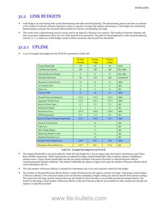
1. IN BULLETS
31.2 LINK BUDGETS
 Link budgets are used during both system dimensioning and radio network planning. The dimensioning process provides an estimate
of the number of network elements required to achieve a specific coverage and capacity performance. Link budgets are used during
dimensioning to estimate the maximum allowed path loss and the corresponding cell range
 The results from a dimensioning exercise can be used as an input for a business case analysis. The number of network elements and
their associated configuration allow the cost of the network to be quantified. The path loss based approach to radio network planning
(section 31.1.1) makes use of link budget results to define maximum allowed path loss thresholds
31.2.1 UPLINK
 A set of example link budgets for the PUSCH is presented in Table 343
PS Data
500 kbps
PS Data
1 Mbps
PS Data
2 Mbps
Channel Bandwidth 20 20 20 MHz
Total Resource Blocks 100 100 100 Res. Blks
Allocated Resource Blocks 8 27 25 Res. Blks
Allocated Subcarriers 96 324 300 Subcarriers
Maximum Transmit Power 23 22 22 dBm
UE Antenna Gain 0 0 0 dBi
Body Loss 0 0 0 dB
Transmit EIRP 23 22 22 dBm
Thermal Noise per Subcarrier -132.2 -132.2 -132.2 dBm
Aggregate Thermal Noise -112.4 -107.1 -107.4 dBm
Receiver Noise Figure 2.5 2.5 2.5 dB
Interference Margin 2 2 2 dB
Interference Floor -107.9 -102.6 -102.9 dBm
SINR Requirement 0.5 -2.0 0.9 dB
Received Signal Strength Requirement -107.4 -104.6 -102.1 dBm
eNode B Antenna Gain 18 dBi
Cable Loss 0 dB
Slow Fading Margin 9 dB
Shadowing Handover Gain 2.5 dB
Building Penetration Loss 18 dB
Isotropic Power Requirement -100.9 -98.1 -95.6 dBm
Maximum Allowed Path Loss 123.9 120.1 117.6 dB
Table 343 – Example link budgets for the PUSCH
 The channel Bandwidth is not used explicitly within the link budget but it has an impact upon the Signal to Interference plus Noise
Ratio (SINR) requirement. SINR requirements are reduced for larger channel bandwidths when frequency domain scheduling is
channel aware. Larger channel bandwidths provide the packet scheduler with greater flexibility to allocate Resource Blocks
experiencing good channel conditions. The channel bandwidth also places an upper limit upon the number of Resource Blocks which
can be allocated to the UE
 The total number of Resource Blocks is included for information and is not used explicitly within the link budget
 The number of allocated Resource Blocks defines a trade-off between the cell capacity and the cell range. Allocating a small number
of Resource Blocks to the connection leads to less air-interface redundancy (higher coding rate and less benefit from channel coding).
This means the cell range must be limited otherwise the eNode B will not be able to successfully decode the transport blocks. The
benefit of allocating a small number of Resource Blocks is that more Resource Blocks are available for other connections and the cell
capacity is typically increased
www.lte-bullets.com

2. LONG TERM EVOLUTION (LTE)
 The example presented in Table 343 allocates 8 Resource Blocks for a 500 kbps connection. Based upon Table 388, a connection with
8 Resource Blocks can use a transport block size of 552 bits to achieve 500 kbps. Table 395 indicates that QPSK is used as a
modulation scheme, which is appropriate for cell edge connections
 The set of 8 Resource Blocks is a relatively large allocation for a transport block size of 552 bits. A single Resource Block allocation
with the normal cyclic prefix can accommodate 2  72 = 144 modulation symbols after accounting for the uplink Demodulation
Reference Signal and the pairing of Resource Blocks in the time domain. This corresponds to a total allocated capacity of 2304 bits
after accounting for all 8 Resource Blocks and the QPSK modulation scheme. The coding rate is then defined by the ratio of 552 /
2304 = 0.24. This represents a low coding rate so the corresponding SINR requirement should be relatively small and the maximum
allowed path loss should be relatively large
 The example presented in Table 343 allocates 27 Resource Blocks for a 1 Mbps connection. Based upon Table 389, a connection with
27 Resource Blocks can use a transport block size of 1192 bits to achieve 1 Mbps. Table 395 indicates that QPSK is used as a
modulation scheme. The corresponding coding rate can be calculated as 1192 / 7776 = 0.15
 The example presented in Table 343 allocates 25 Resource Blocks for a 2 Mbps connection. Based upon Table 389, a connection with
25 Resource Blocks can use a transport block size of 2216 bits to achieve 2 Mbps. Table 395 indicates that QPSK is used as a
modulation scheme. The corresponding coding rate can be calculated as 2216 / 7200 = 0.31
 The number of allocated subcarriers is given by 12  the number of allocated Resource Blocks. The number of allocated subcarriers is
used when aggregating the total thermal noise received by the BTS, i.e. it defines the noise bandwidth
 The maximum transmit power of 23 dBm corresponds to the capability of UE power class 3 specified by 3GPP within TS 36.101. This
capability has a tolerance of  2 dB so 23 dBm could be optimistic for some devices. The maximum transmit power has been reduced
to 22 dBm for the 1 Mbps and 2 Mbps examples because 3GPP TS 36.101 specifies a 1 dB Maximum Power Reduction (MPR) when
more than 18 Resource Blocks are allocated from the 20 MHz channel bandwidth while using QPSK
 The terminal antenna gain can vary from one UE model to another. Datacards may have a higher antenna gain than handheld devices.
UE typically have an antenna gain in the order of 0 dBi
 Body loss is dependent upon the relative positions of the UE, the end-user and the serving cell. A figure of 3 dB is typically assumed
when the UE is held to one side of the end-user’s head. A figure of 0 dB is typically assumed when the UE is positioned away from
the body
 The first main result from the uplink link budget is the transmit Effective Isotropic Radiated Power (EIRP). This is defined using the
expression below:
Transmit EIRP = Maximum Transmit Power + UE Antenna Gain – Body Loss
 The thermal noise per subcarrier quantifies the noise power within the bandwidth of a single 15 kHz subcarrier. This is calculated
using 10  LOG(kTB), where k is the Boltzmann constant (1.38  10-23
), T is the temperature (290 Kelvin) and B is the bandwidth
(15000 Hz)
 The aggregate thermal noise quantifies the noise power within the total allocated bandwidth. It is given by the thermal noise per
subcarrier + 10  LOG(number of allocated subcarriers)
 The receiver noise figure assumption reflects the performance of the eNode B receiver subsystem. The noise figure belonging to the
eNode B cabinet should be used if the receiver subsystem does not include a Mast Head Amplifier (MHA). If an MHA is included, the
noise figure should be the composite noise figure of the MHA, cable/connectors and eNode B cabinet. The composite noise figure can
be calculated using Friis’ equation:













CableMHA
eNodeB
MHA
cable
MHA
GainGain
NF
Gain
NF
NFLOGComposite
11
10FigureNoise
 With the exception of the composite noise figure result, all of the variables within the preceding equation have linear units. The noise
figure of the cable and connectors is equal to their loss. For example, the noise figure is 2 dB in log units and 1.6 in linear units if the
cable and connector loss is 2 dB. The gain of the cable and connectors is equal to -1  their loss, i.e. -2 dB in log units and 0.6 in linear
units. Friis’ equation illustrates that when the MHA has a high gain, the noise figure of the receiver sub-system is dominated by the
noise figure of the MHA. This emphasises the importance of having a low noise, high gain amplifier for the MHA
 The interference margin is generated by co-channel interference from UE served by neighbouring cells. The interference margin is
likely to be greater in urban areas where the site density is relatively high. Heterogeneous network architectures can also lead to
increased co-channel interference. Inter-Cell Interference Coordination (ICIC) is intended to help manage levels of co-channel
interference
 The interference floor is defined using the expression below:
Interference Floor = Aggregate Thermal Noise + Receiver Noise Figure + Interference Margin
 The Signal to Interference plus Noise Ratio (SINR) requirement is defined by link level simulations which model the BTS receiver
performance when the allocated transport block size is transferred using the allocated number of Resource Blocks with a specific
www.lte-bullets.com

3. IN BULLETS
Block Error Rate (BLER). Link level simulations model a specific propagation channel so the SINR requirement is specific for that
channel. Propagation channel modelling includes fast fading (unless it is a static channel) so the resultant SINR includes the impact of
fast fading
 The SINR examples in Table 343 do not demonstrate an obvious trend between SINR requirement and bit rate requirement, i.e. the
500 kbps example has a higher SINR requirement than the 1 Mbps example, but a lower SINR requirement than the 2 Mbps example.
This results from the different Resource Block allocations and different coding rates. The SINR requirement increases as the coding
rate increases
 The second main result from the uplink link budget is the Received Signal Strength Requirement. This is defined using the expression
below:
Received Signal Strength Requirement = Interference Floor + SINR Requirement
 As expected, the Received Signal Strength Requirement increases as the bit rate requirement increases. The higher interference floors
associated with the larger Resource Block allocations increase the resultant Received Signal Strength Requirement
 The eNode B antenna gain should be representative of the antenna type planned for network deployment. In practice, networks may
include a range of antenna types. Antenna gains tend to decrease as the horizontal and vertical beamwidths increase and the antenna
becomes less directional
 The antenna gain figure can incorporate a polarisation loss of approximately 0.5 dB. Antenna gains are typically quoted from
measurements which have been recorded using a receiving antenna element which has exactly the same polarisation as the
transmitting antenna element. In practice, the two antenna elements have different polarisations and a polarisation loss is experienced.
Reflections change the polarision of a radio signal and this helps to reduce the loss because many signals with different polarisations
can reach the receiving antenna. Cross polar antennas also reduce the potential for polarisation loss because the maximum angular
offset is 45 compared to 90 for a vertically polarised antenna
 The cable loss variable within the uplink link budget is only applicable if it has not already been included as part of the receiver noise
figure. The uplink cable loss is included within the composite noise figure if an MHA has been assumed. Otherwise, the cable loss
should equal all cable and connector losses between the eNode B cabinet and antenna. The example presented in Table 343 assumes
an MHA is used so the cable loss is set to 0 dB
 The slow fading margin is calculated from an indoor location probability and an indoor standard deviation. The indoor location
probability is often specified as an average probability of experiencing indoor coverage across the cell area. This figure is translated to
an equivalent cell edge indoor coverage probability before combining with the standard deviation to generate the slow fading margin.
The indoor location probability at cell edge will be less than the average as a result of the higher UE transmit power requirement. The
indoor standard deviation represents a combination of the outdoor standard deviation associated with slow fading, and the standard
deviation generated by the variance of the building penetration loss
 The shadowing handover gain is generated by allowing the UE to handover onto the best server. When the UE is at cell edge and there
are multiple potential serving cells, the UE is able select the best cell to help avoid experiencing fades. The shadowing handover gain
is reduced when handovers have hysteresis to avoid ping-pongs between cells. The shadowing handover gain would reduce to 0 dB at
the edge of network coverage where there are no neighbouring cells to act as handover candidates. This may also be the case at some
indoor locations
 Including the building penetration loss as part of the link budget generates an outdoor maximum allowed path loss result which
includes sufficient margin to allow UE at the cell edge to establish and maintain connections from within buildings. The building
penetration loss may be replaced by a vehicle penetration loss if link budgets are generated for a section of motorway or a rural area
 The assumptions for building penetration loss typically depend upon the environment type, e.g. building penetration could be greater
within an urban environment than within a suburban environment. The building penetration loss usually represents the link budget
assumption with the greatest uncertainty. SINR figures and shadowing handover gains could have an uncertainty of  1 dB while
building penetration loss could have an uncertainty of  5 dB. This uncertainty is included within the link budget result by calculating
the slow fading margin from an indoor standard deviation which incorporates the variance of the building penetration loss. Building
penetration loss assumptions are relatively difficult to validate in the field due to the large variance between different buildings and the
geometry of those buildings with respect to the radio network plan
 The third main result from the uplink link budget is the Isotropic Power Requirement. This is defined using the expression below:
Isotropic Power Requirement = Received Signal Requirement – eNode B antenna Gain + Cable Loss +
Slow Fading Margin – Shadowing Handover Gain + Building Penetration Loss
 The Maximum Allowed Path Loss is then calculated as the difference between the transmit EIRP and the isotropic power requirement:
Maximum Allowed Path Loss = Transmit EIRP – Isotropic Power Requirement
 This maximum allowed path loss result can be compared with the equivalent downlink result to determine whether coverage is uplink
or downlink limited. This comparison requires an offset to account for the frequency difference between the uplink and downlink
frequency bands. Higher frequencies tend to experience greater path loss so coverage will tend to be downlink limited if both the
uplink and downlink link budgets generate equal maximum allowed path loss results. The frequency dependant term within a typical
Okumura-Hata path loss model is given by the equation below:
www.lte-bullets.com