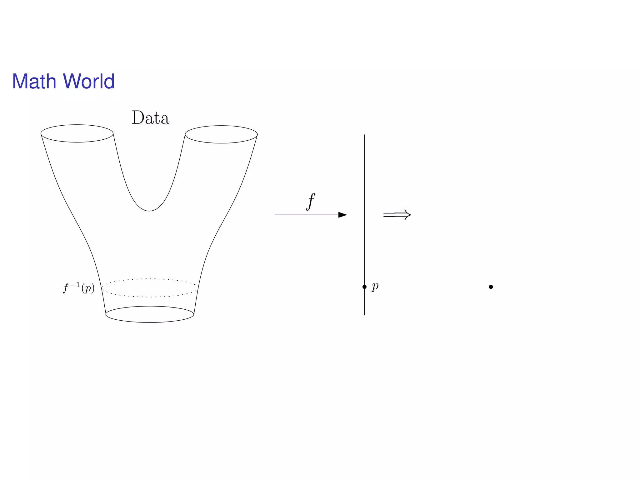
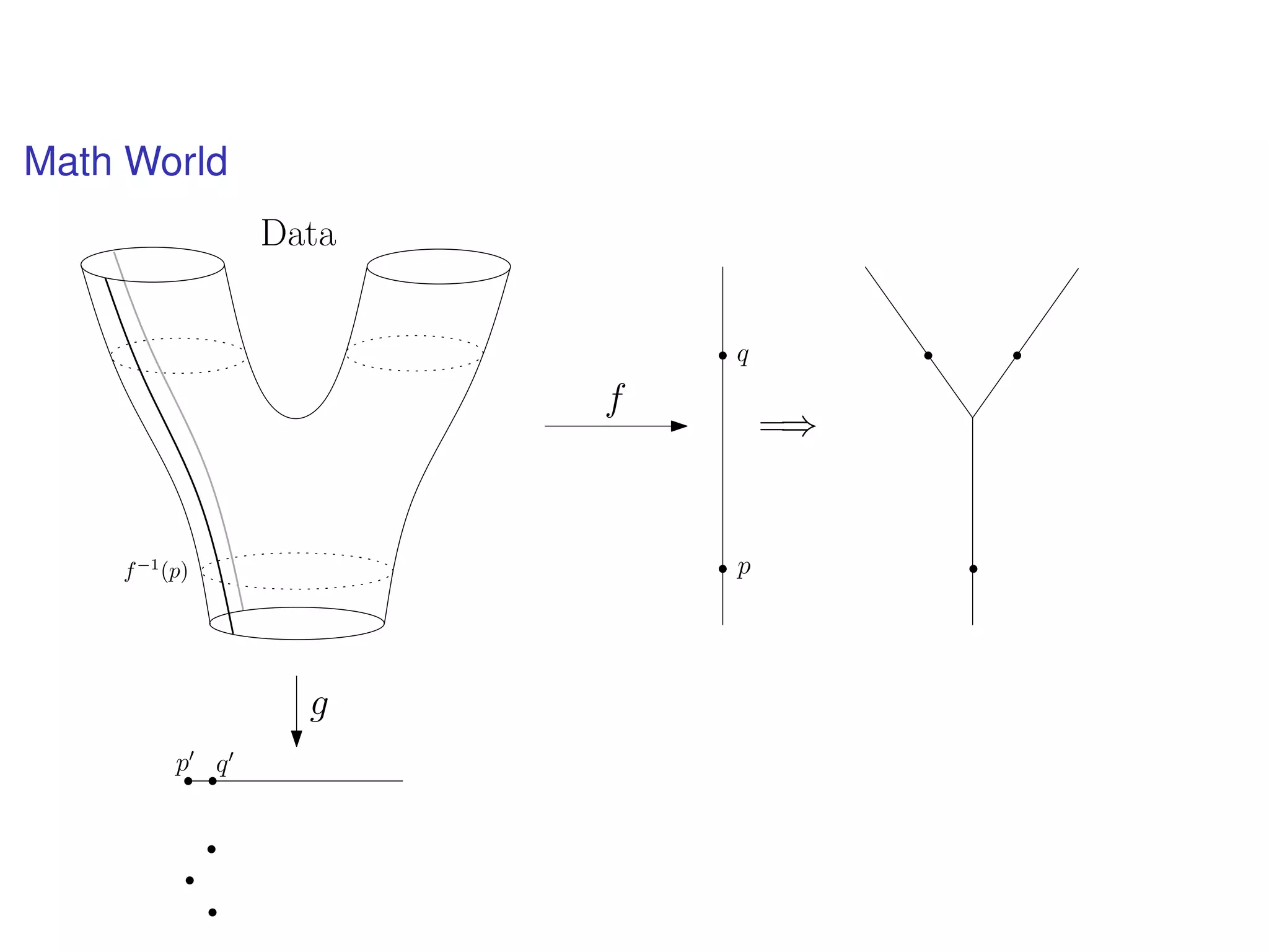
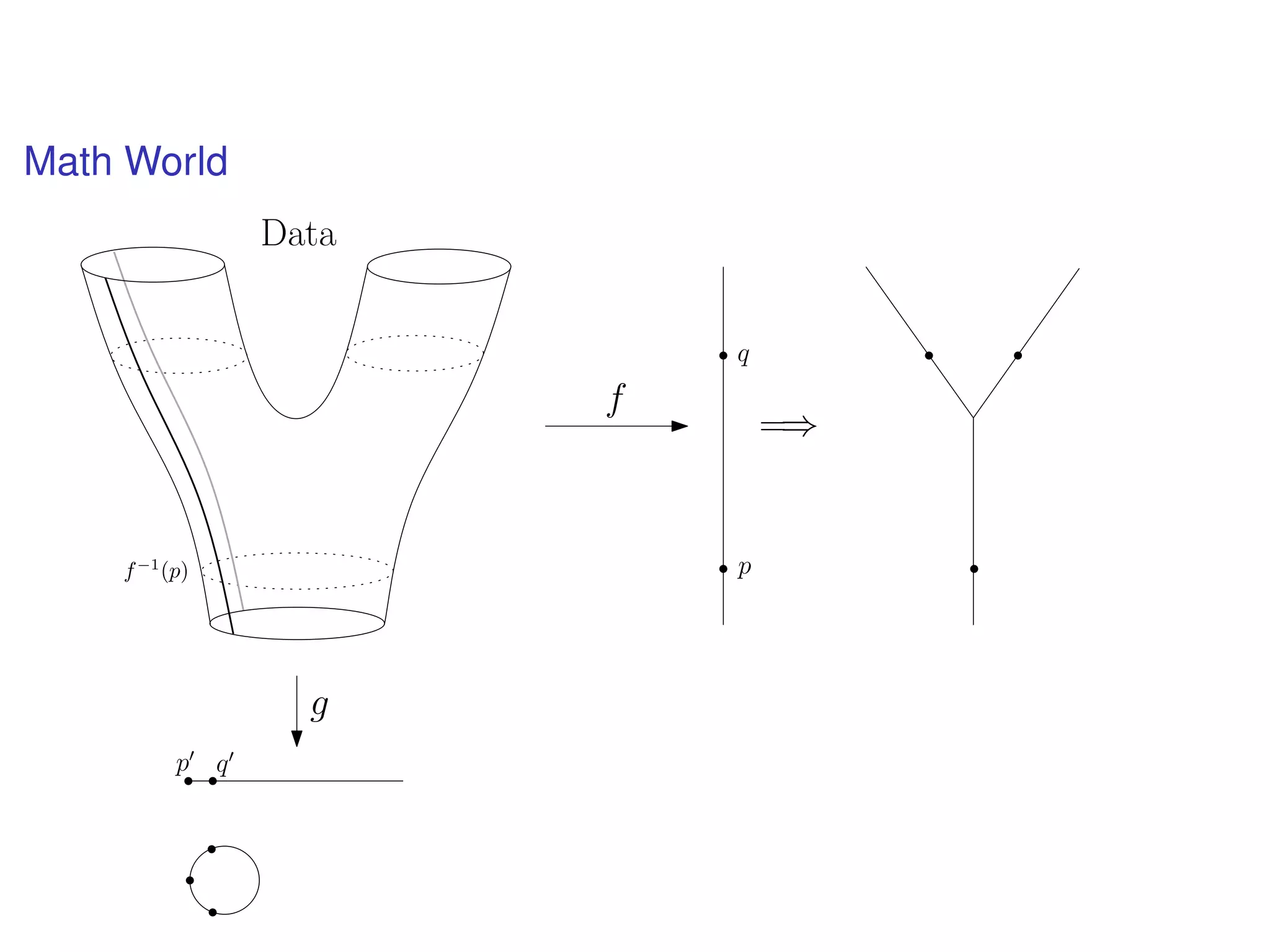
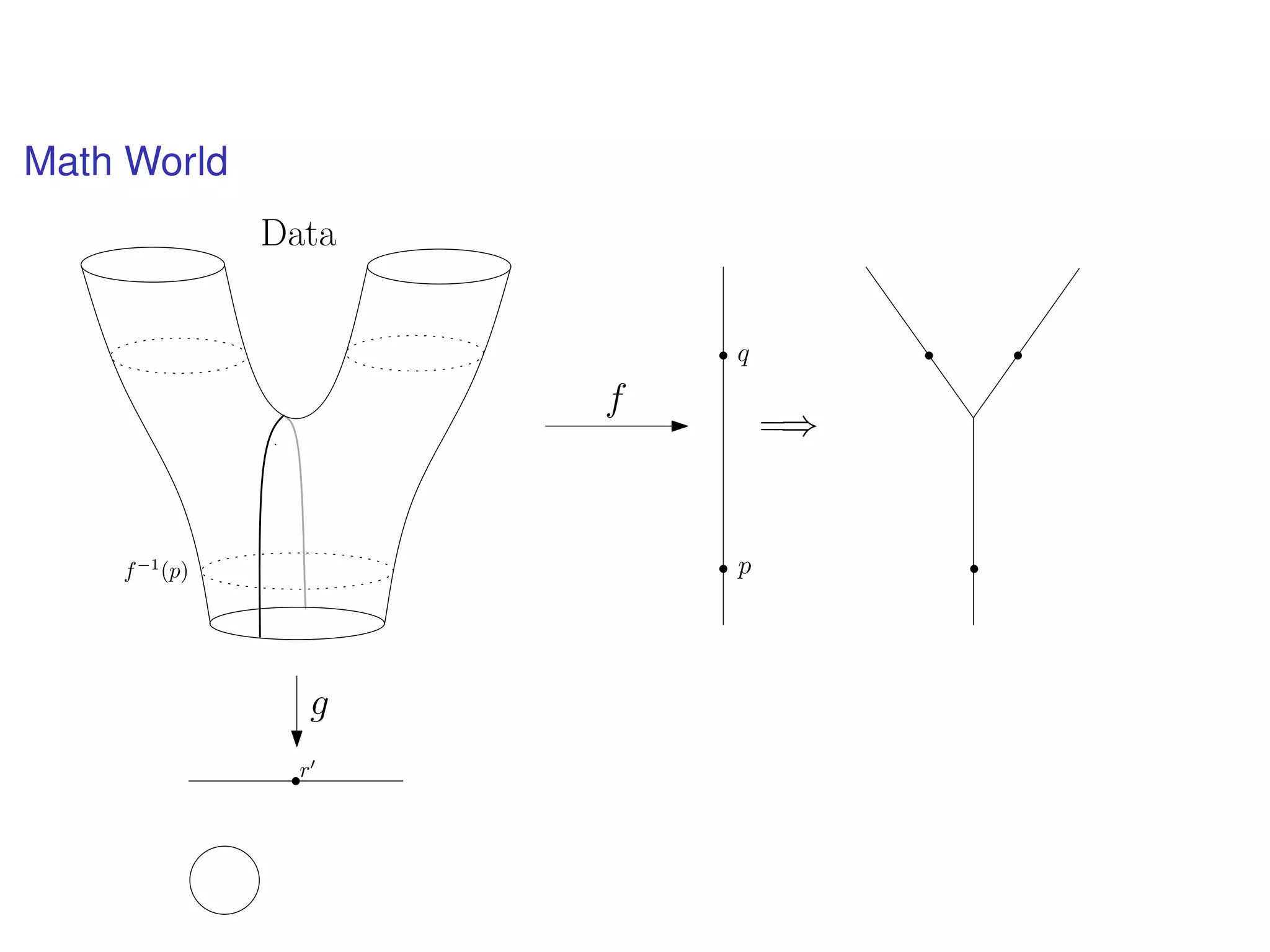
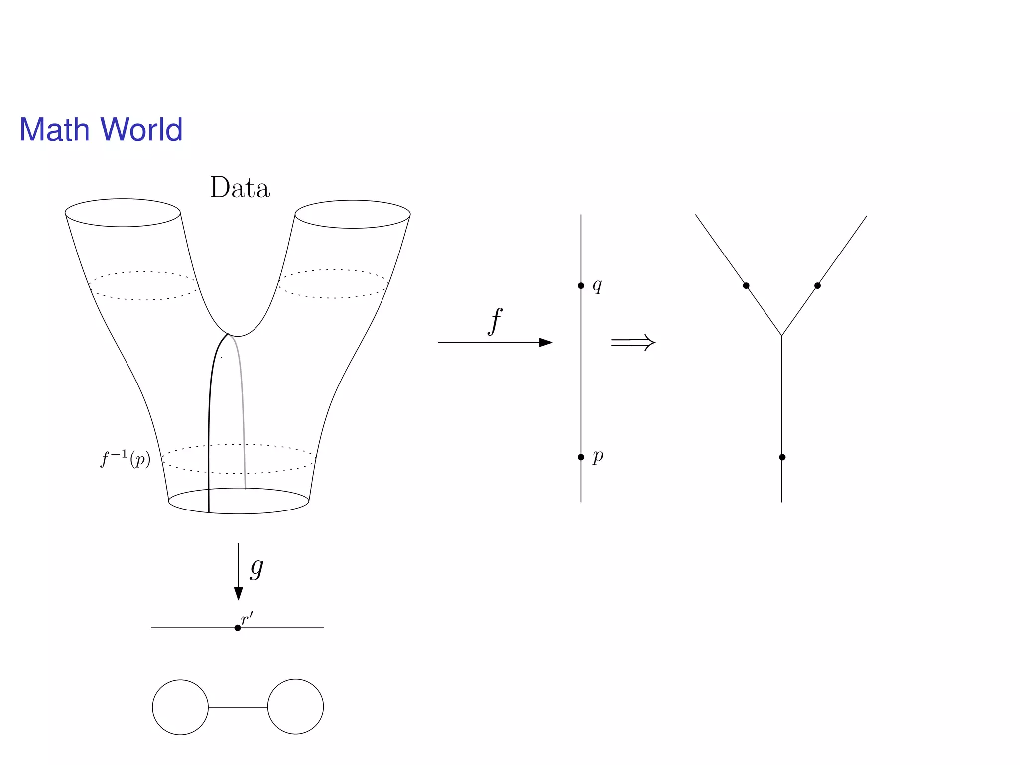
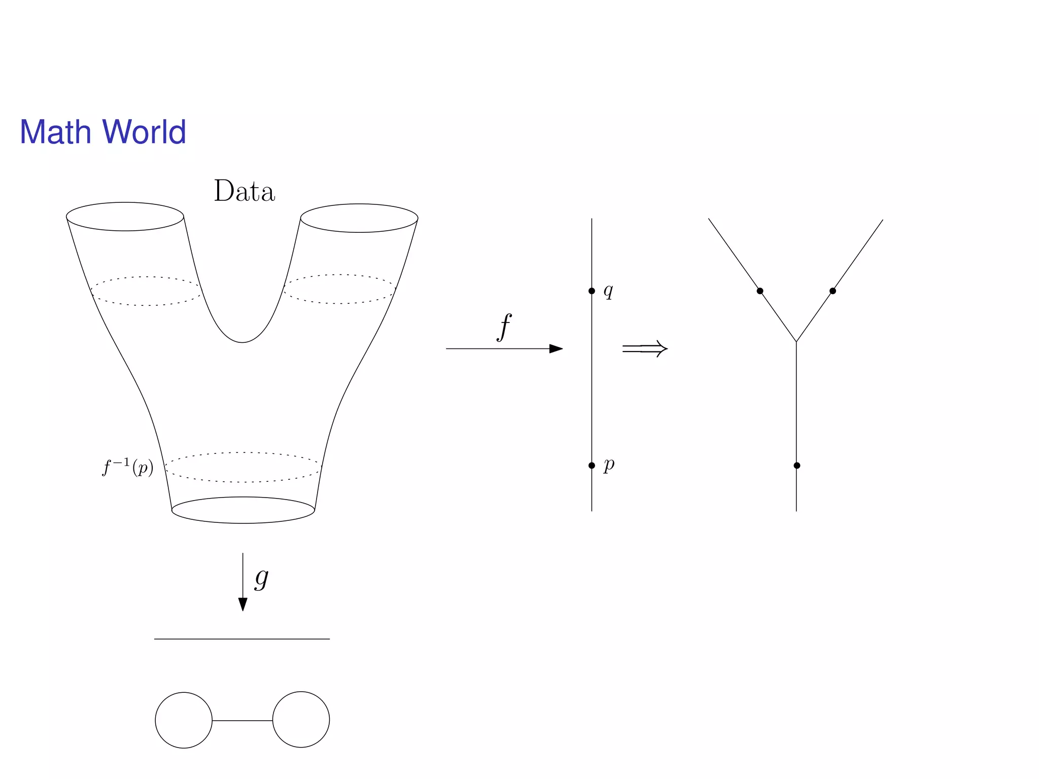
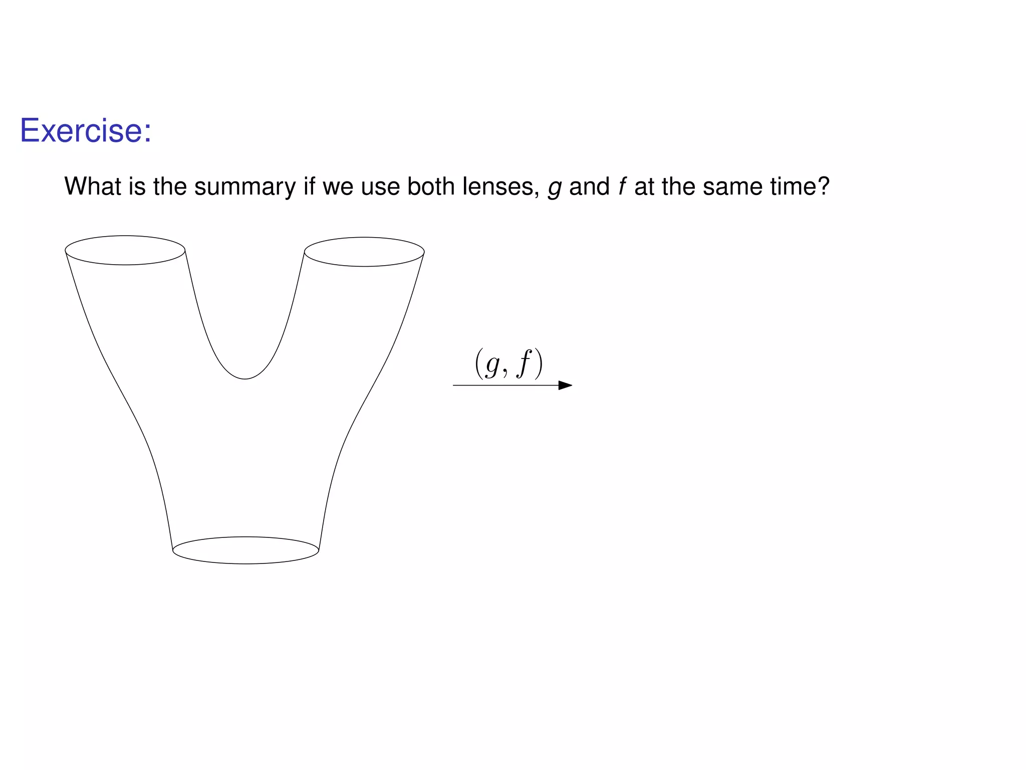
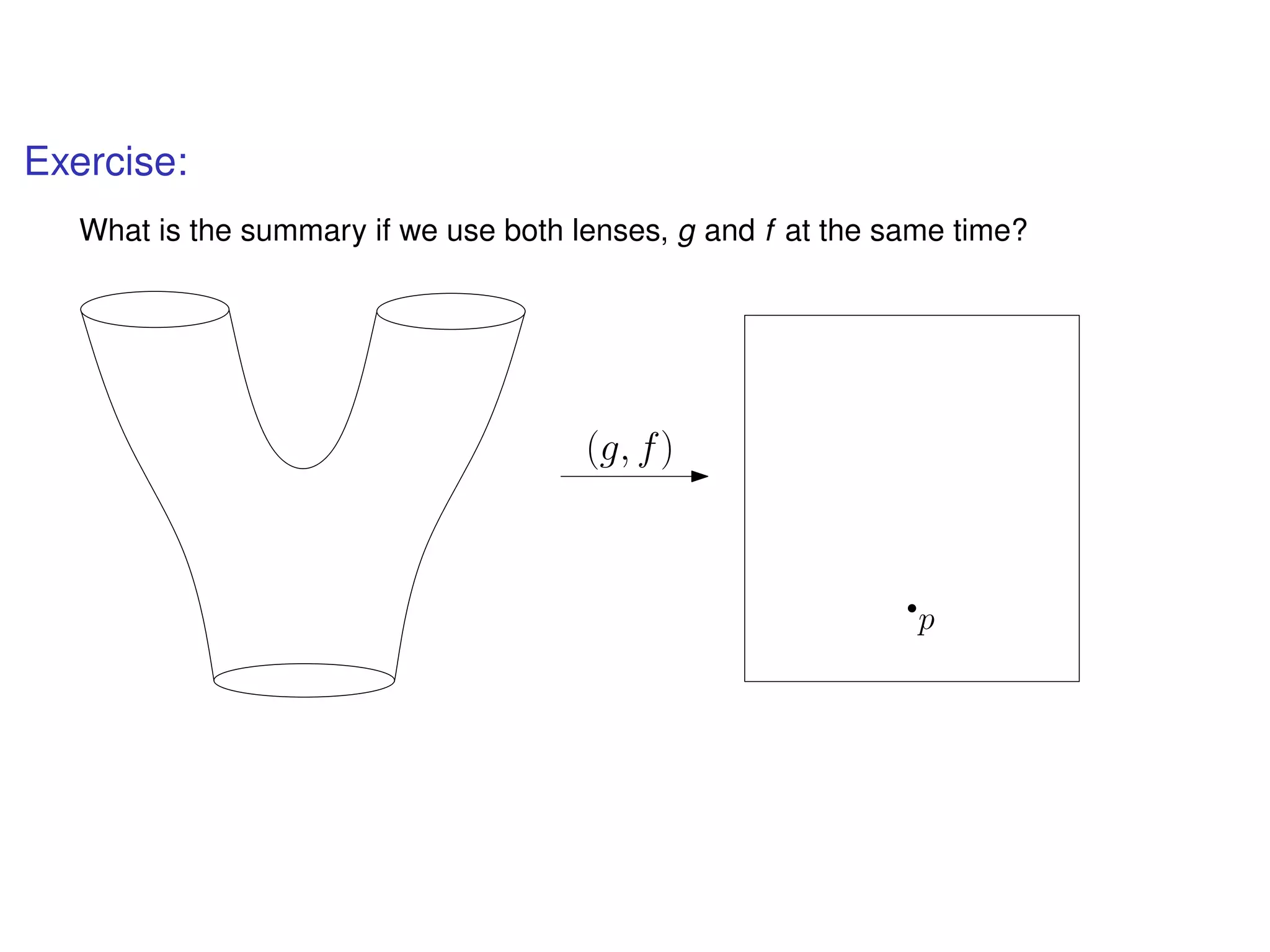
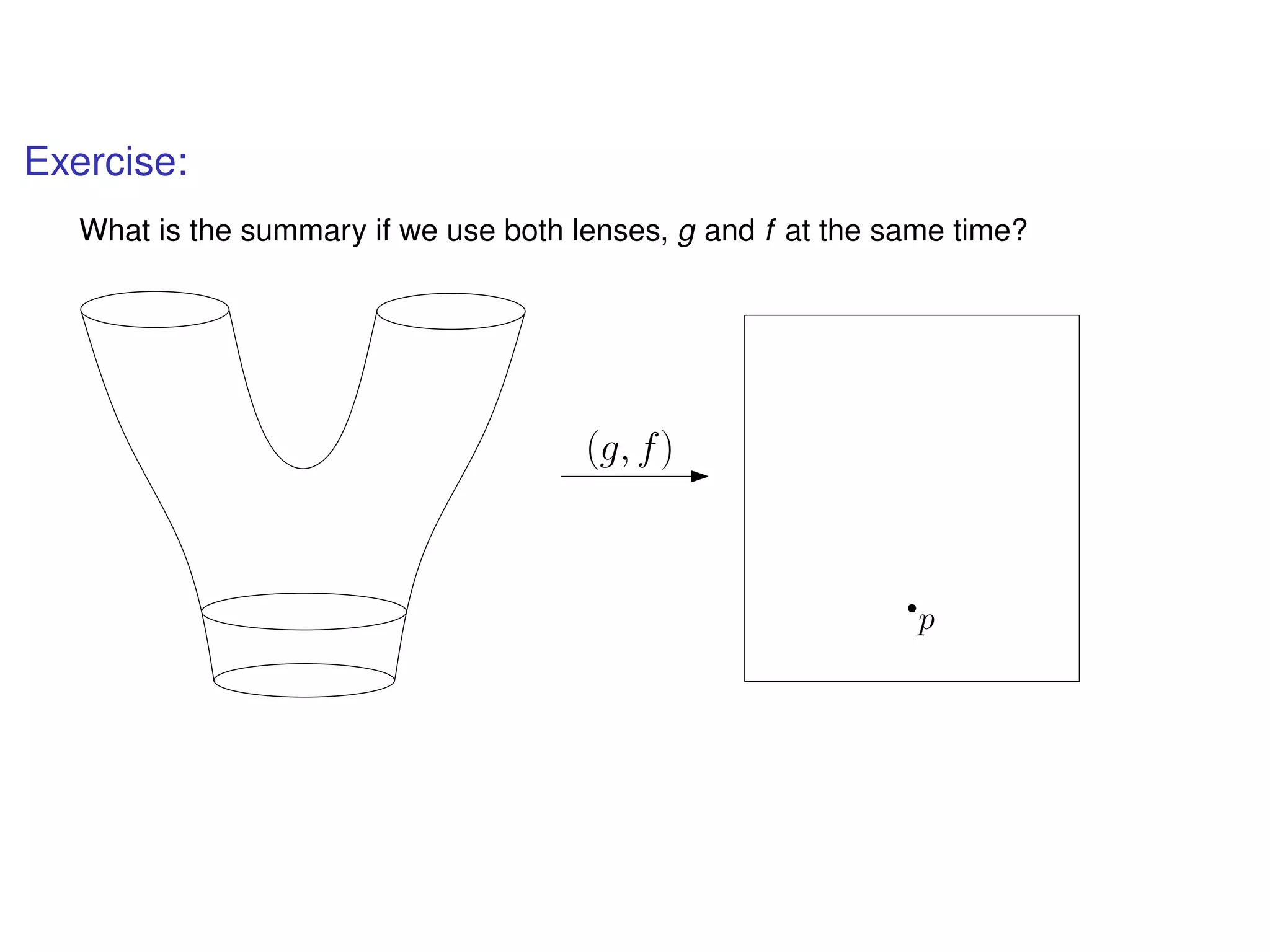
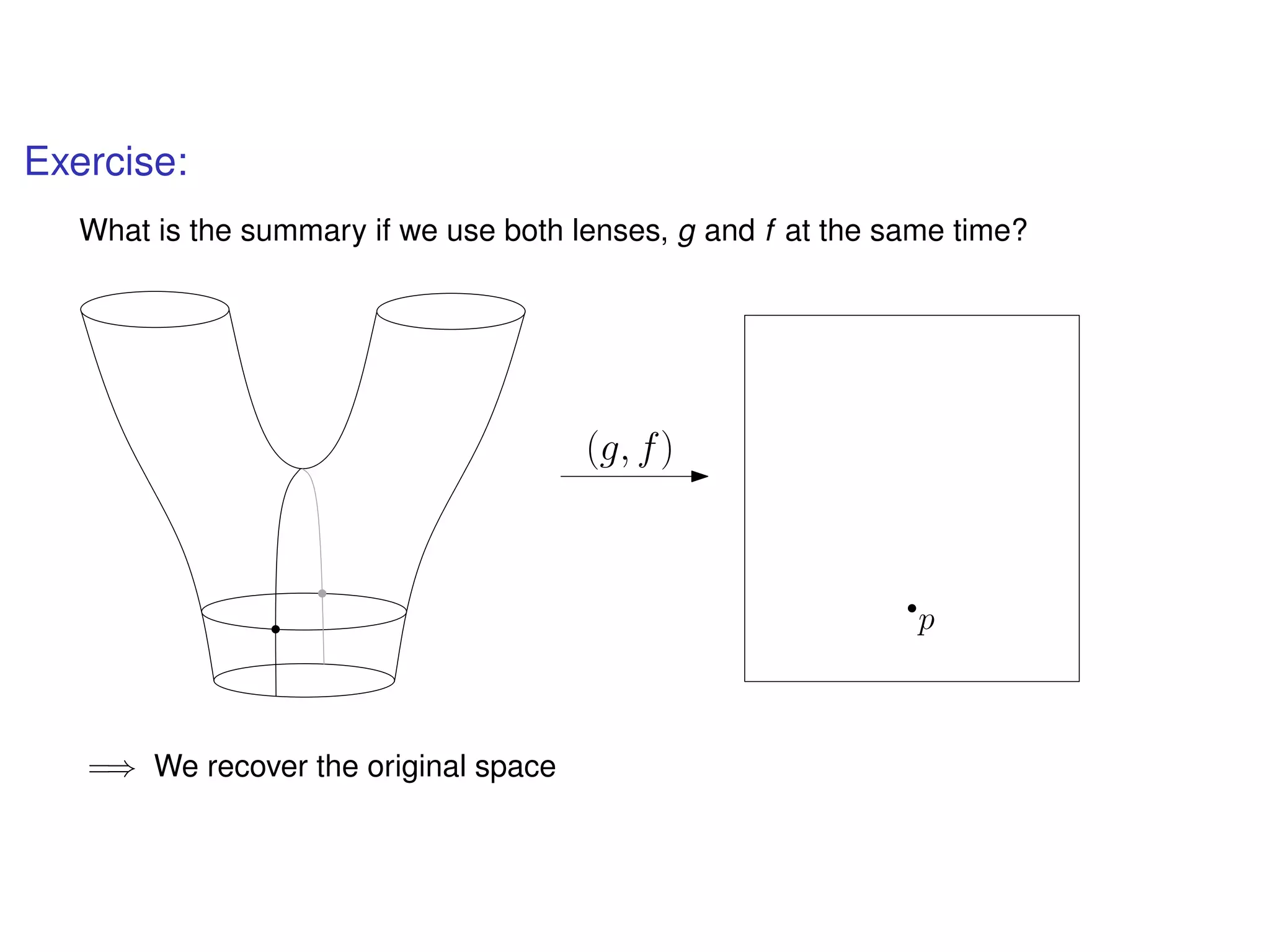
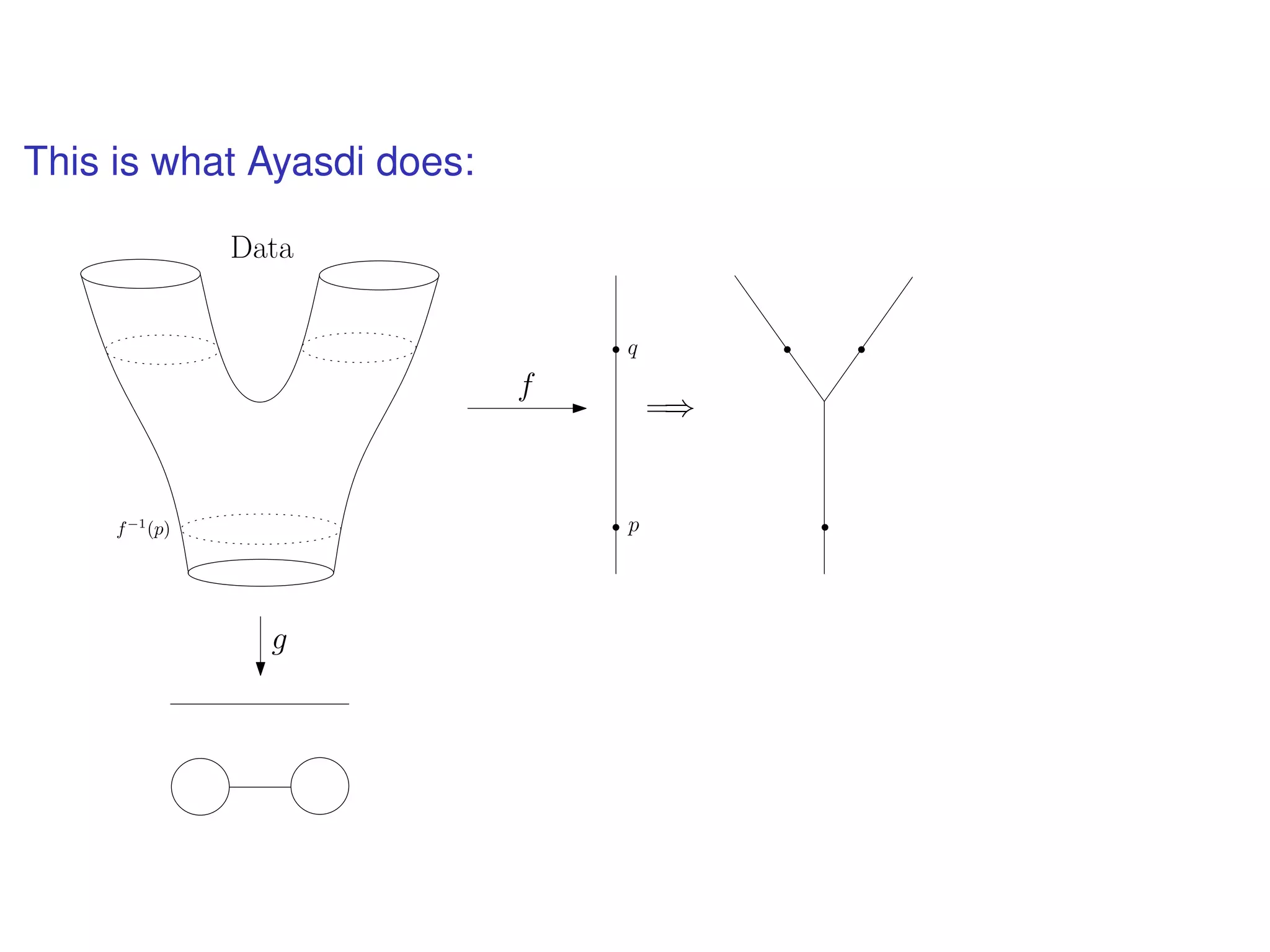
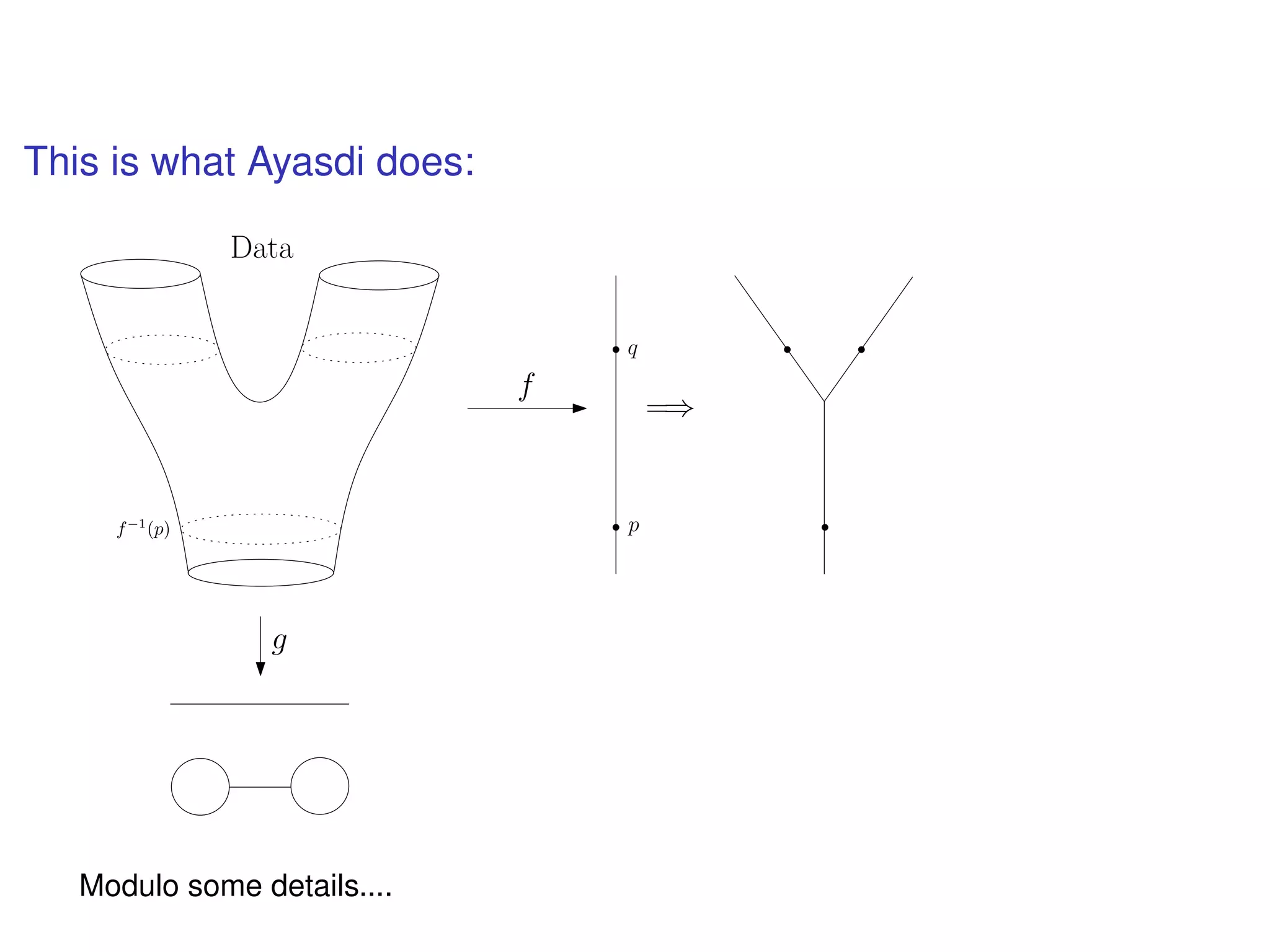
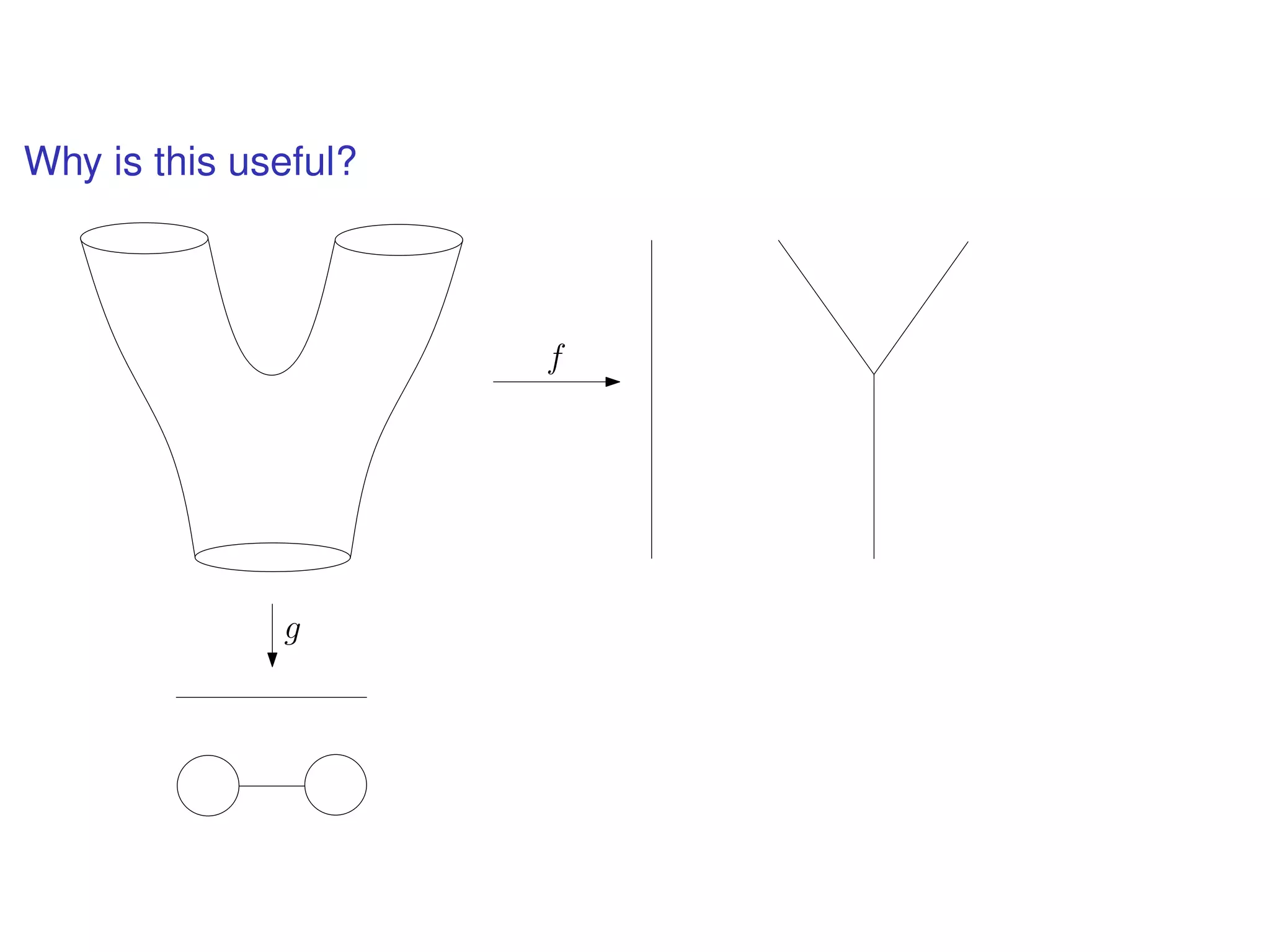
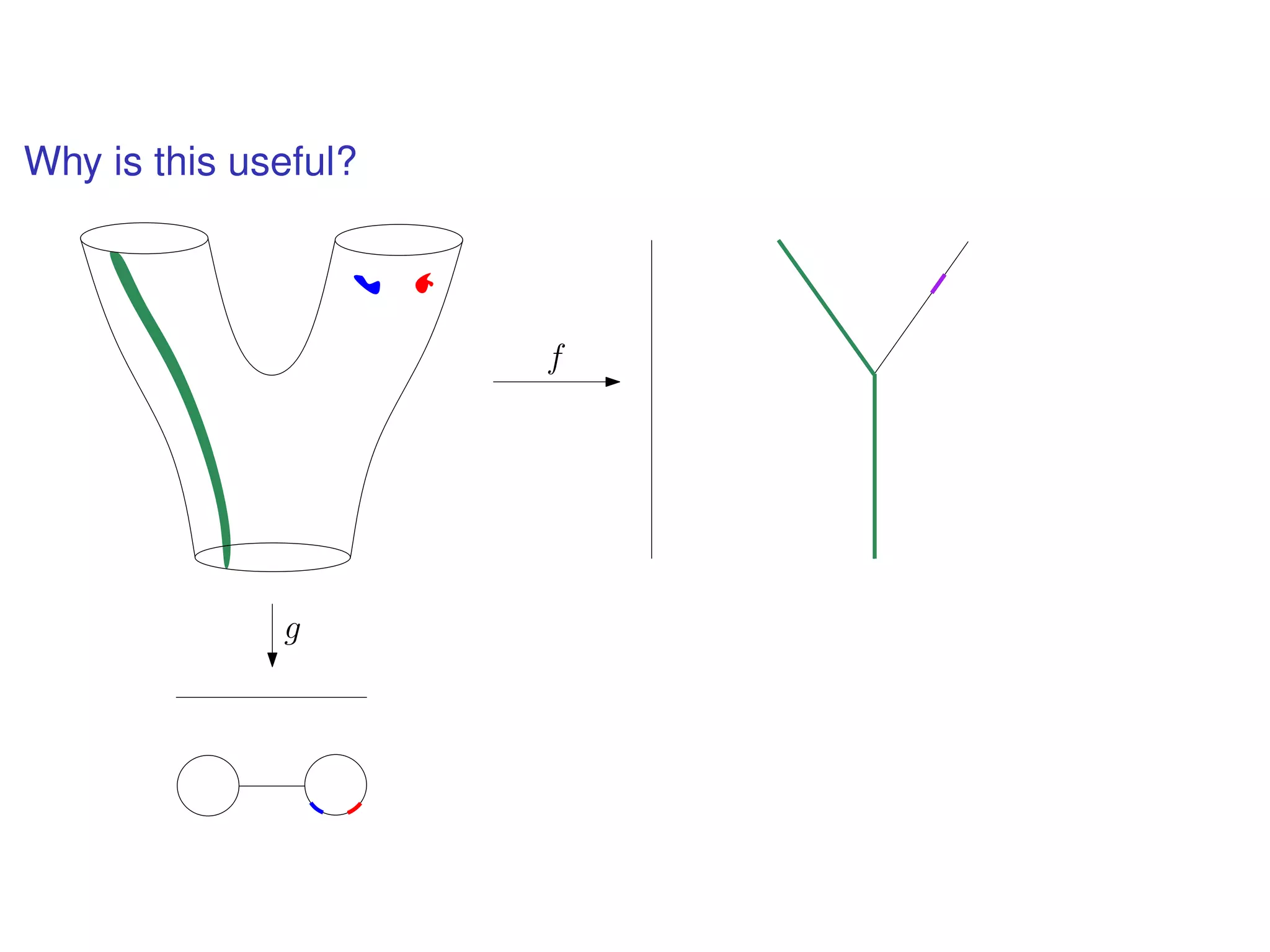
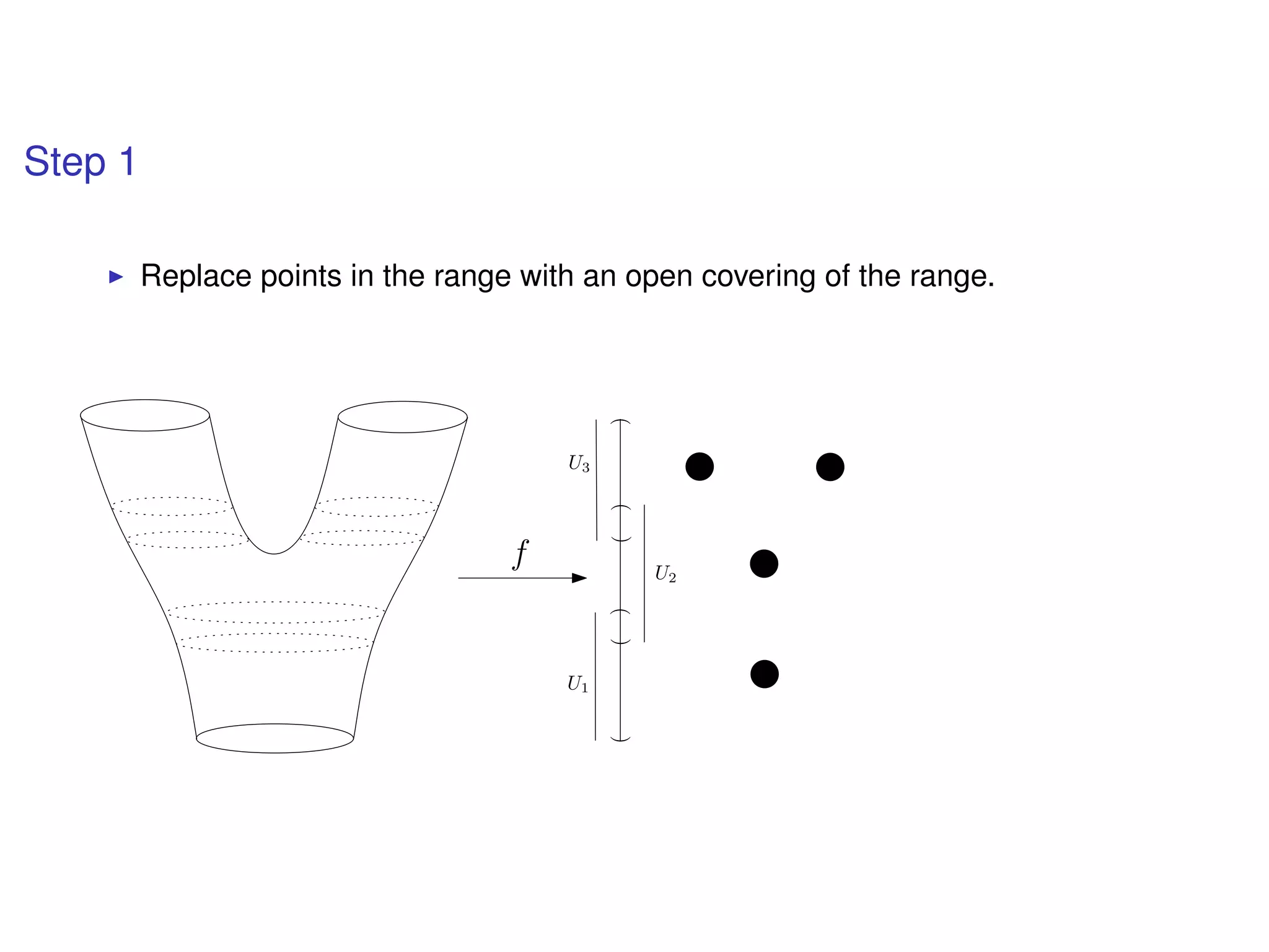
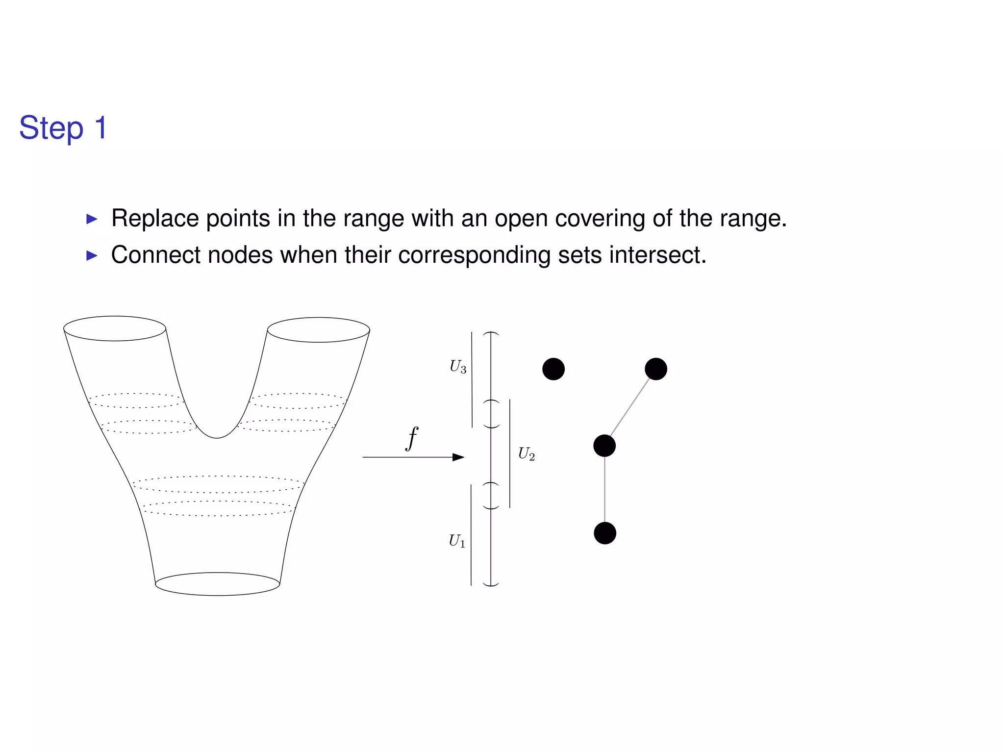
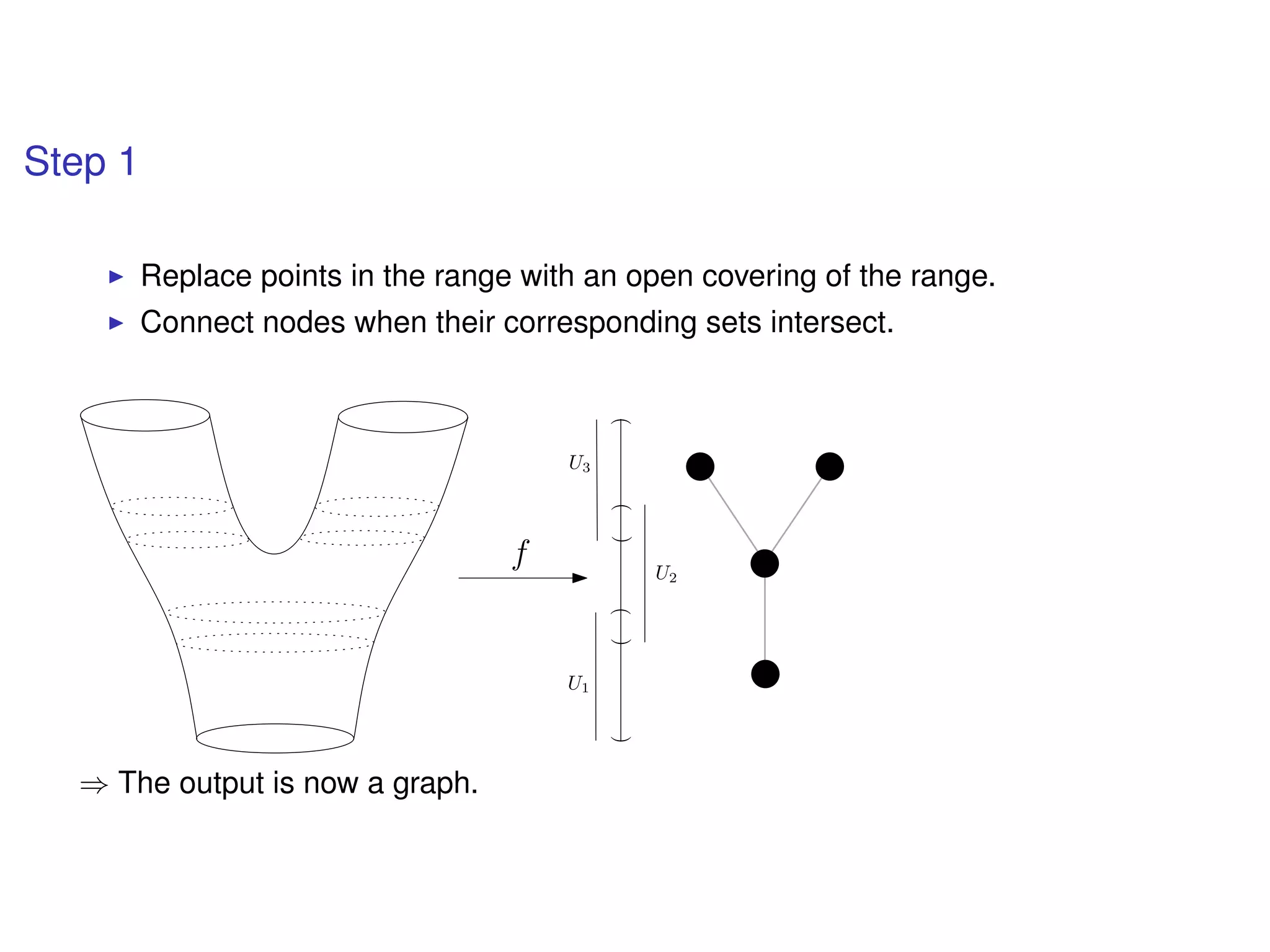
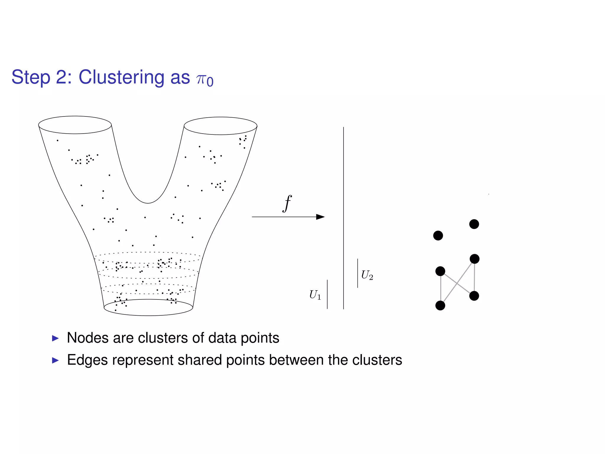
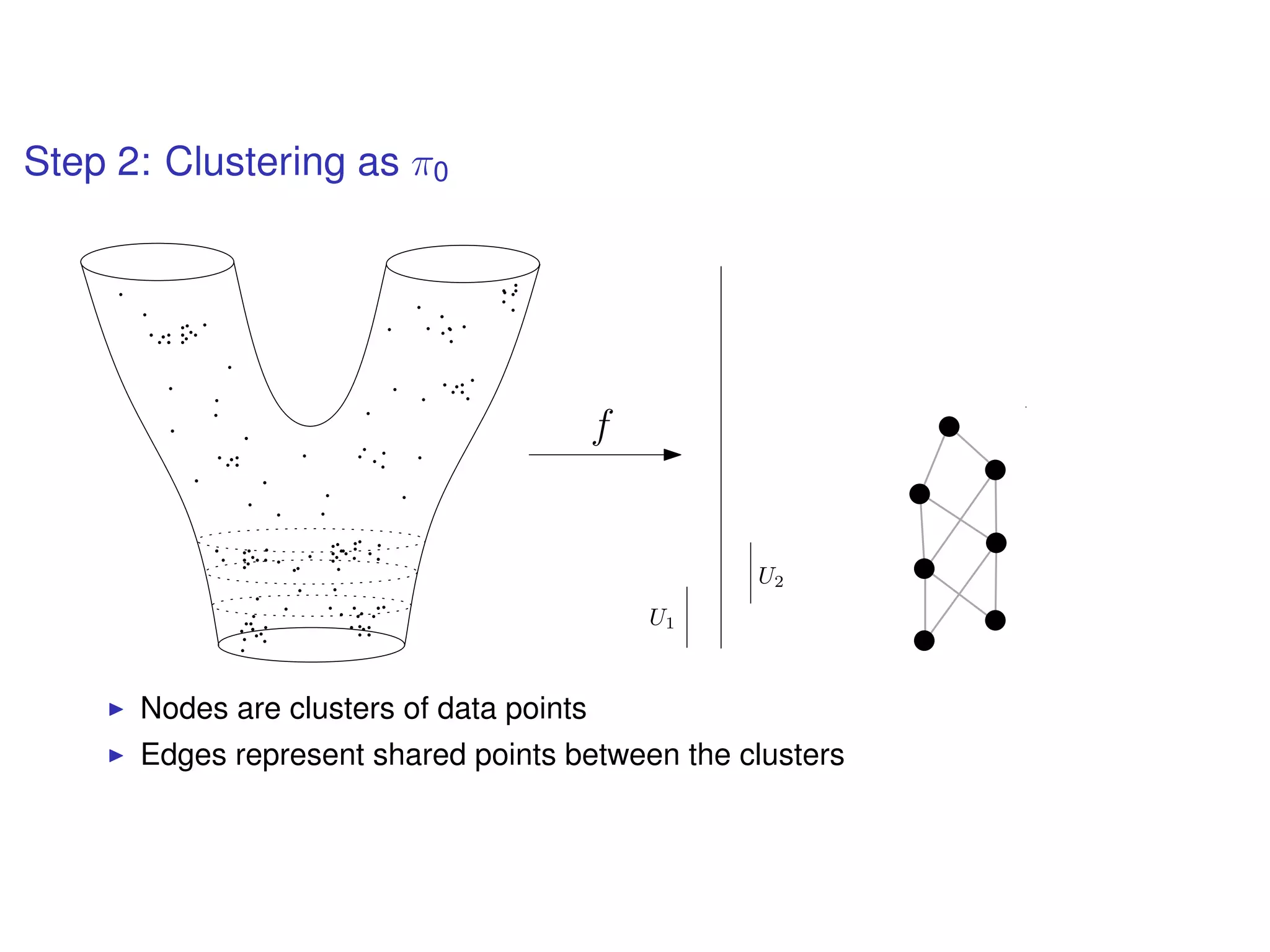
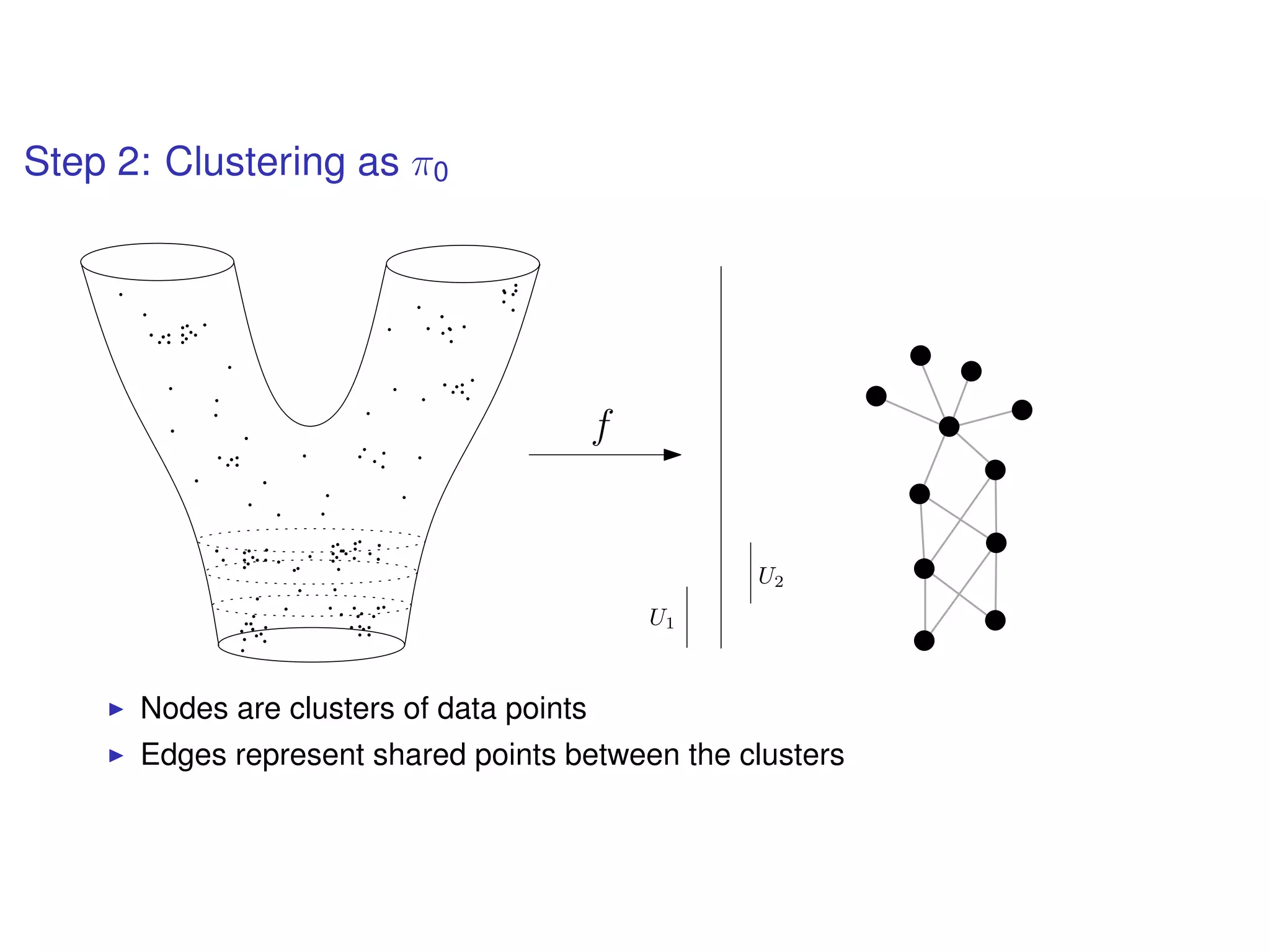
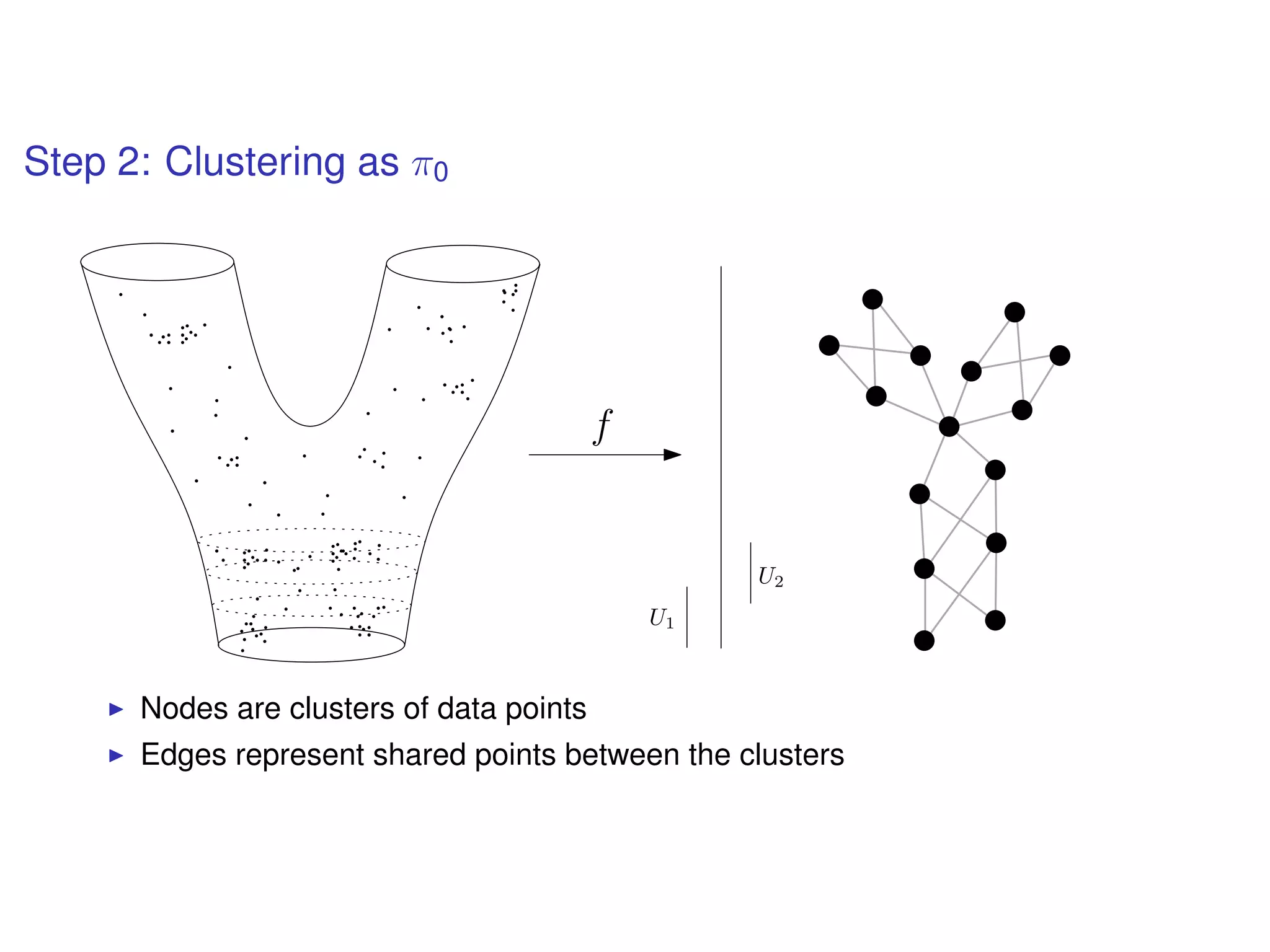
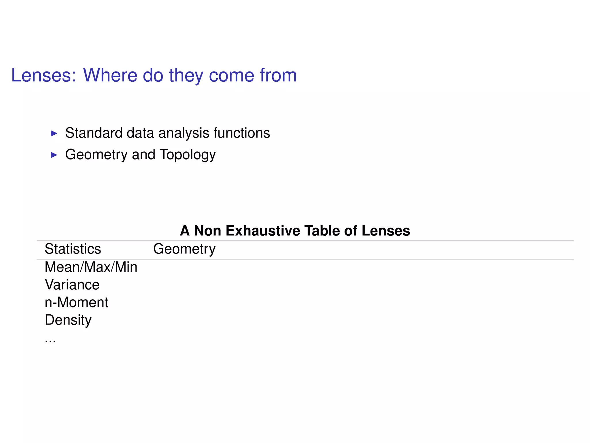
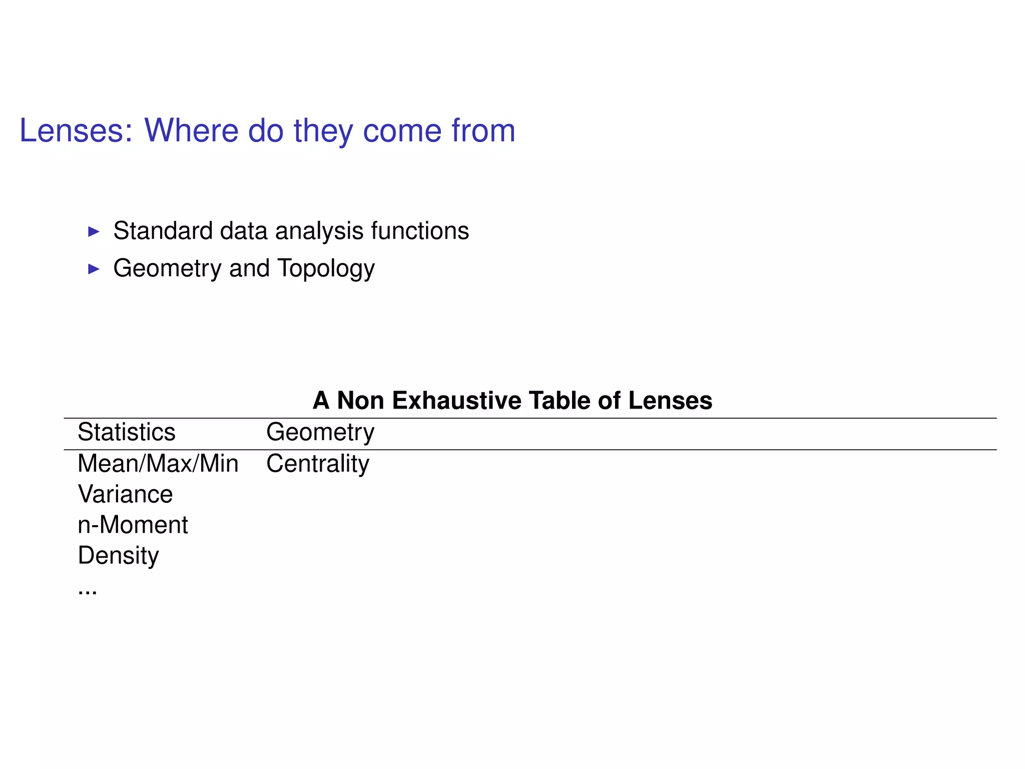
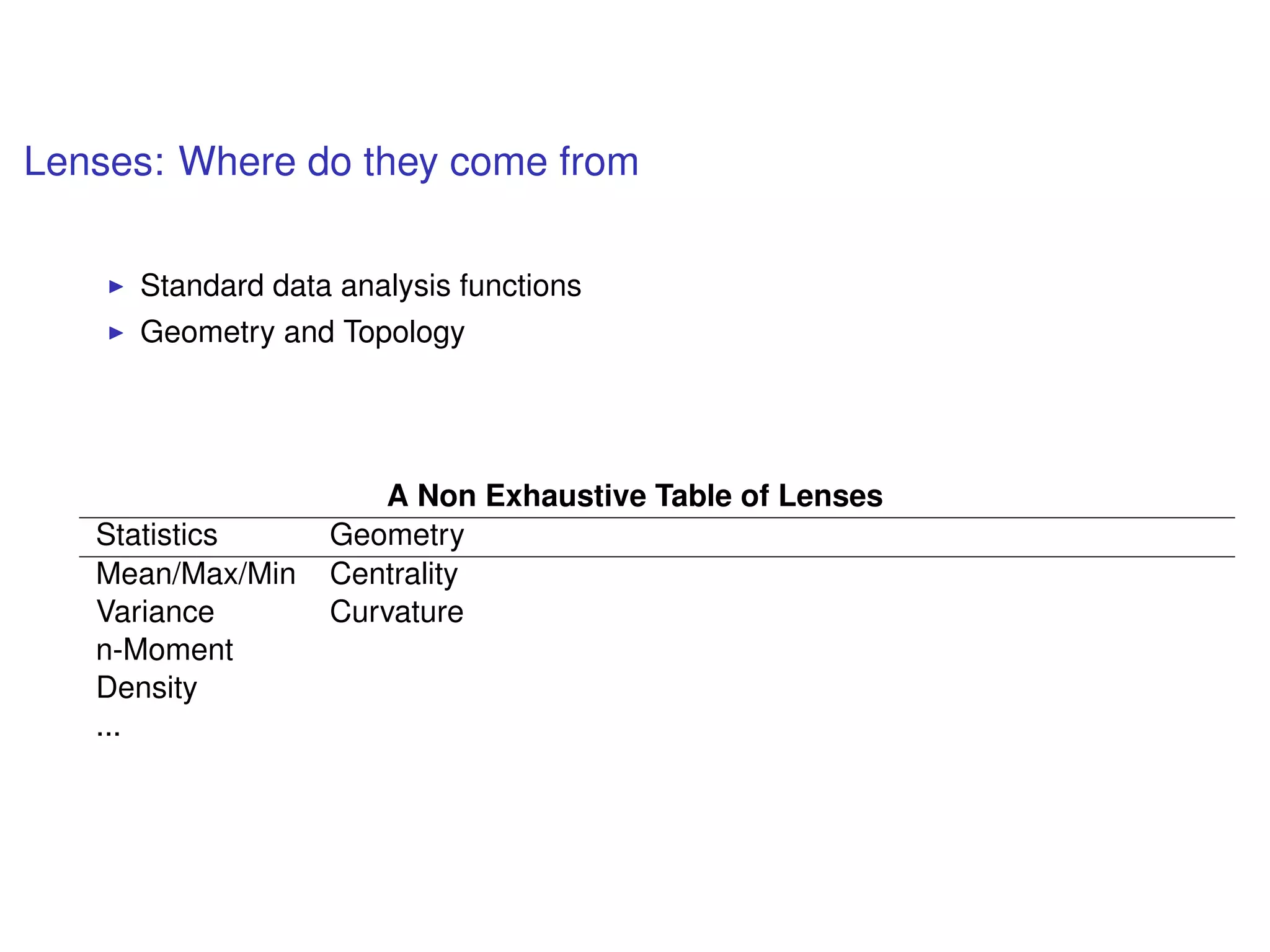
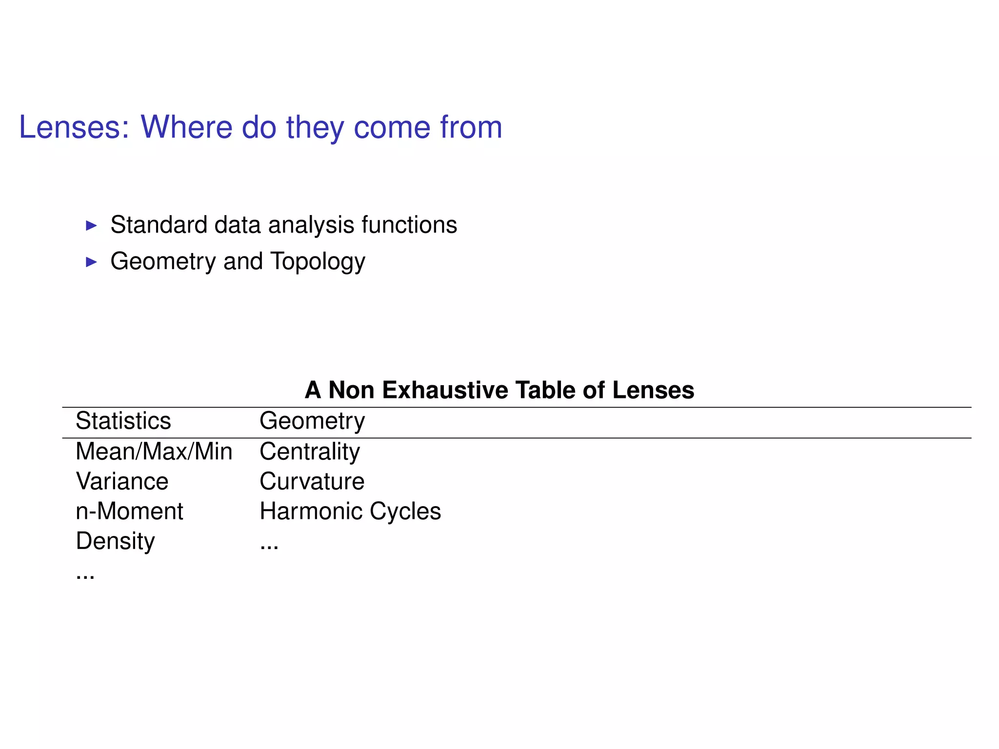
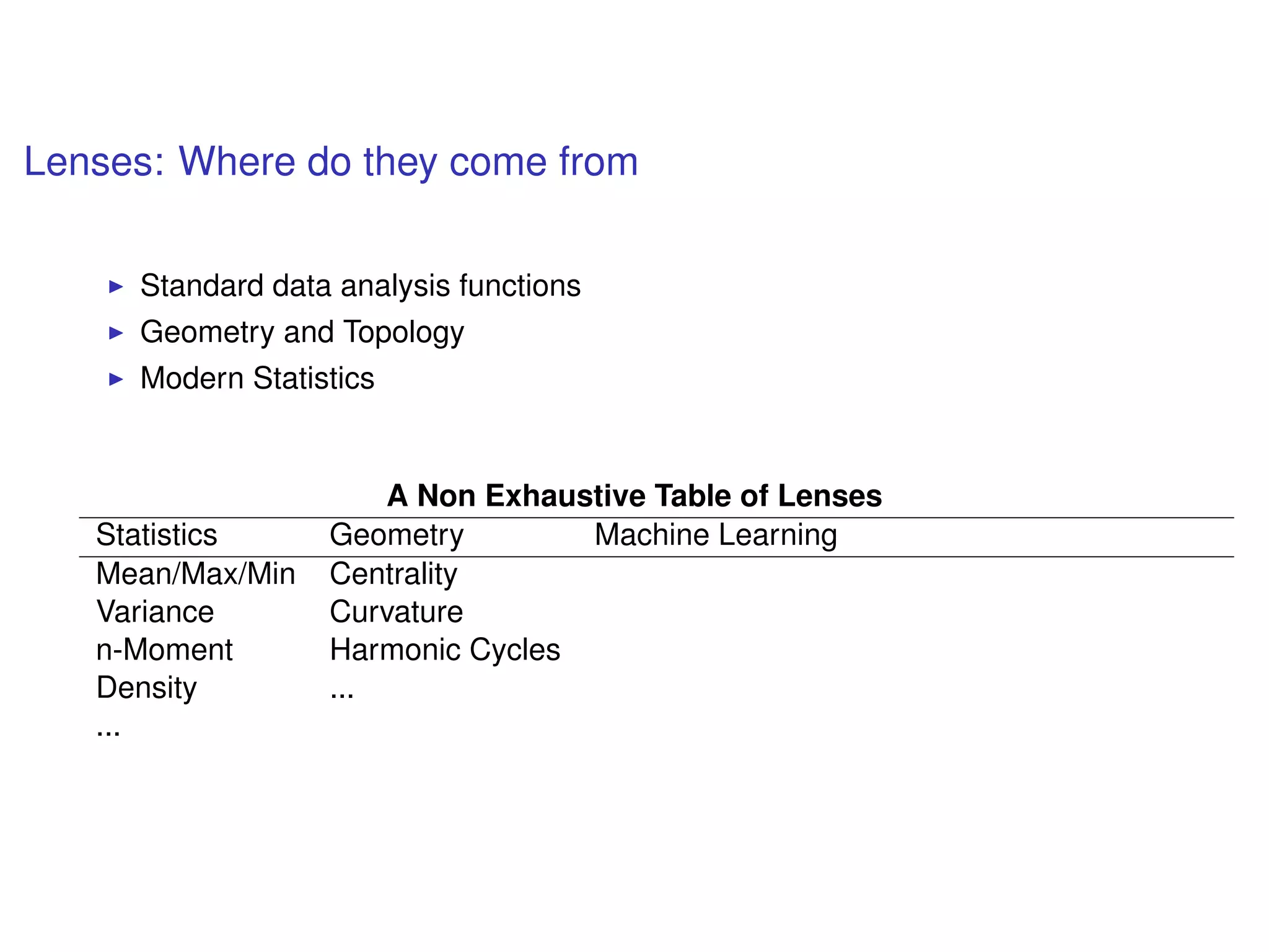
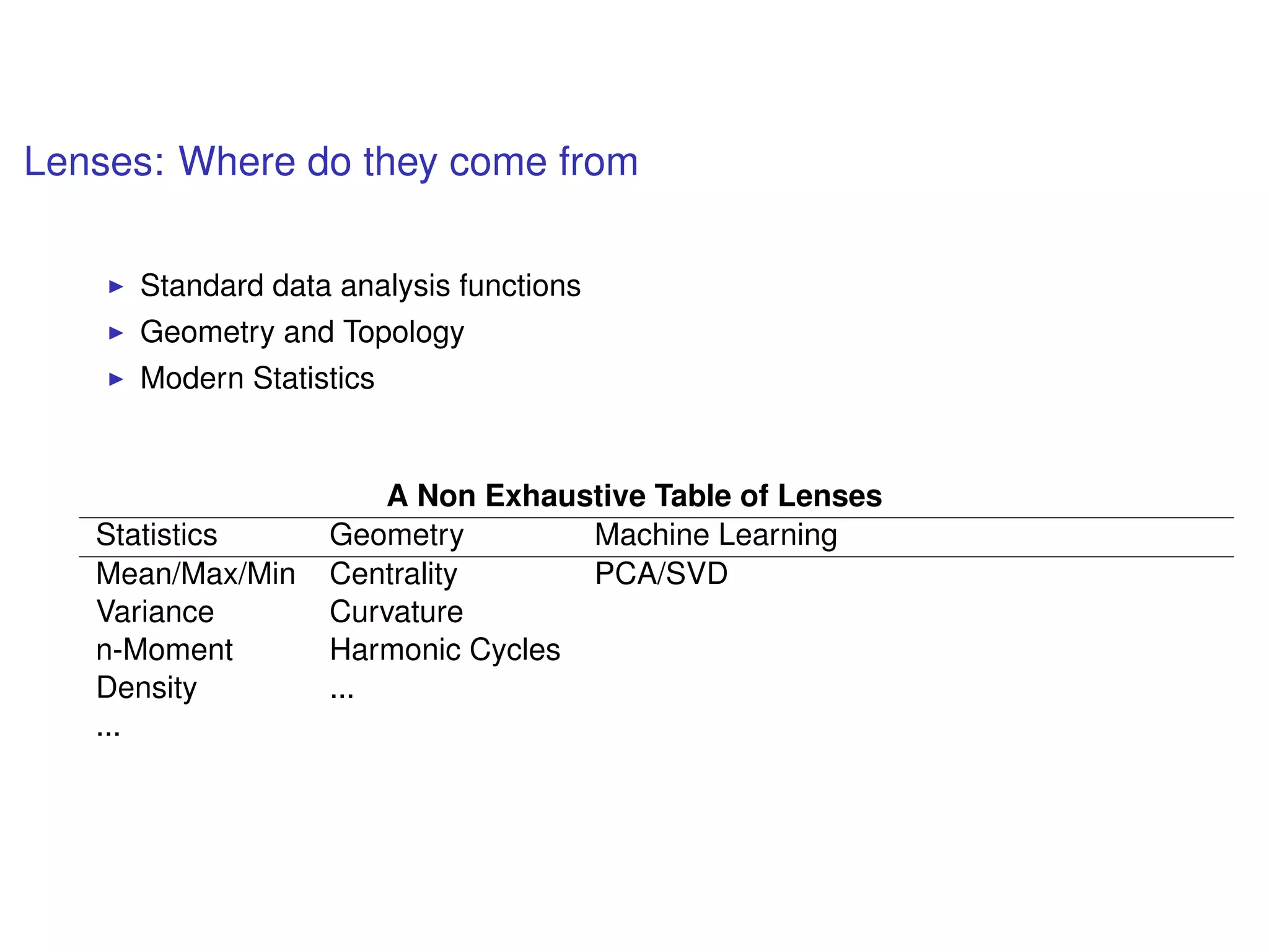
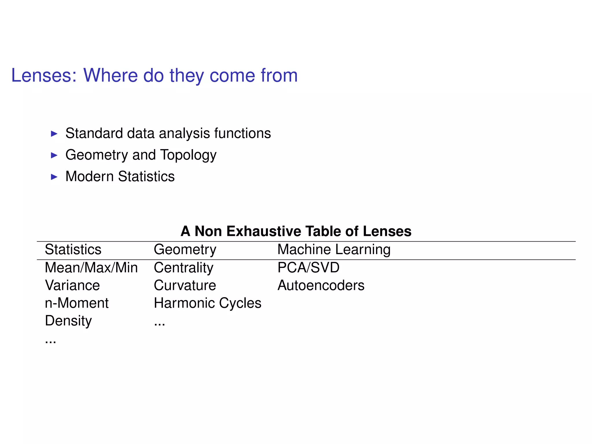
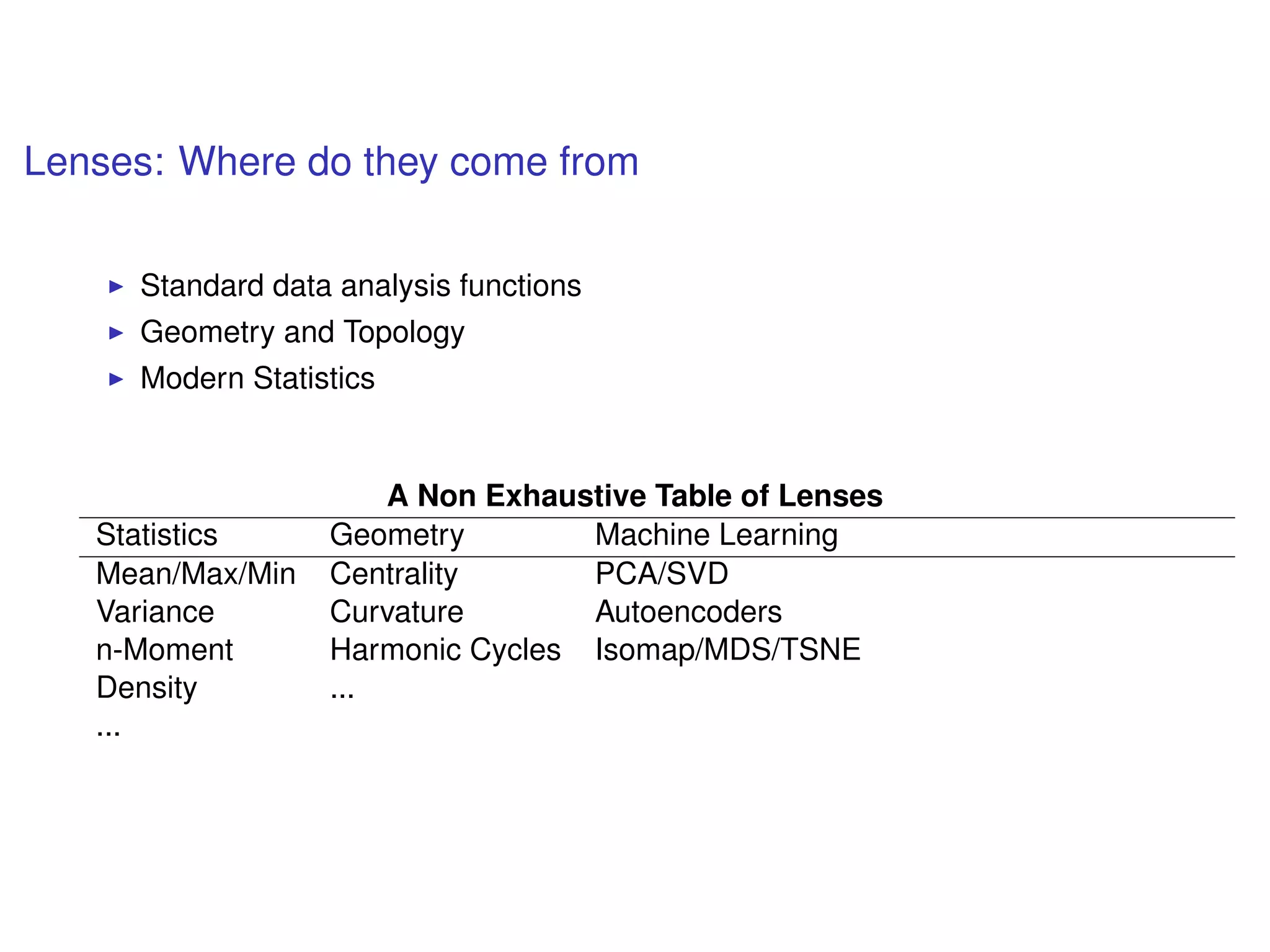
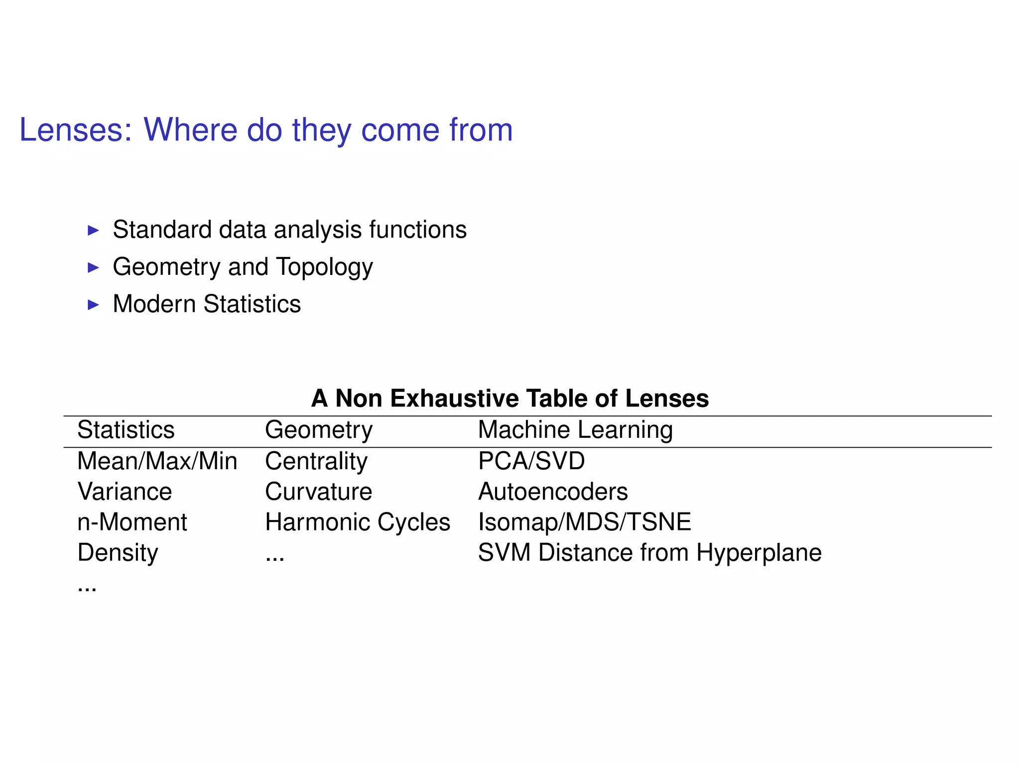
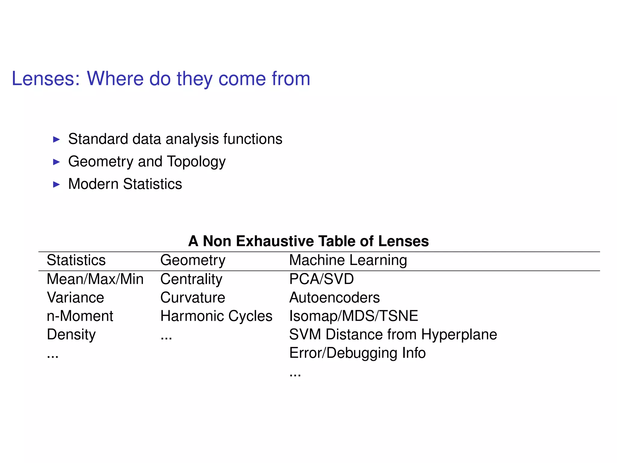
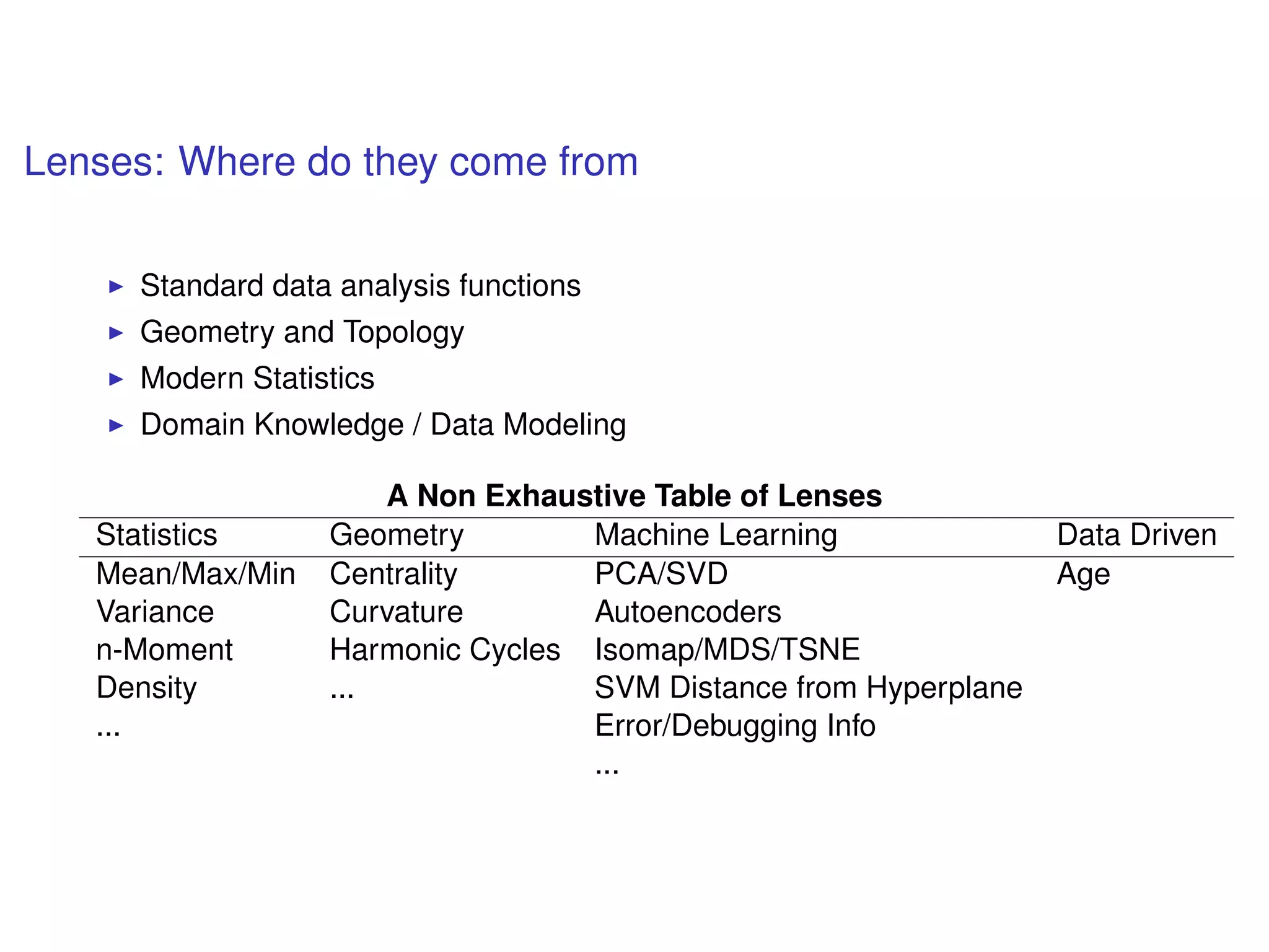
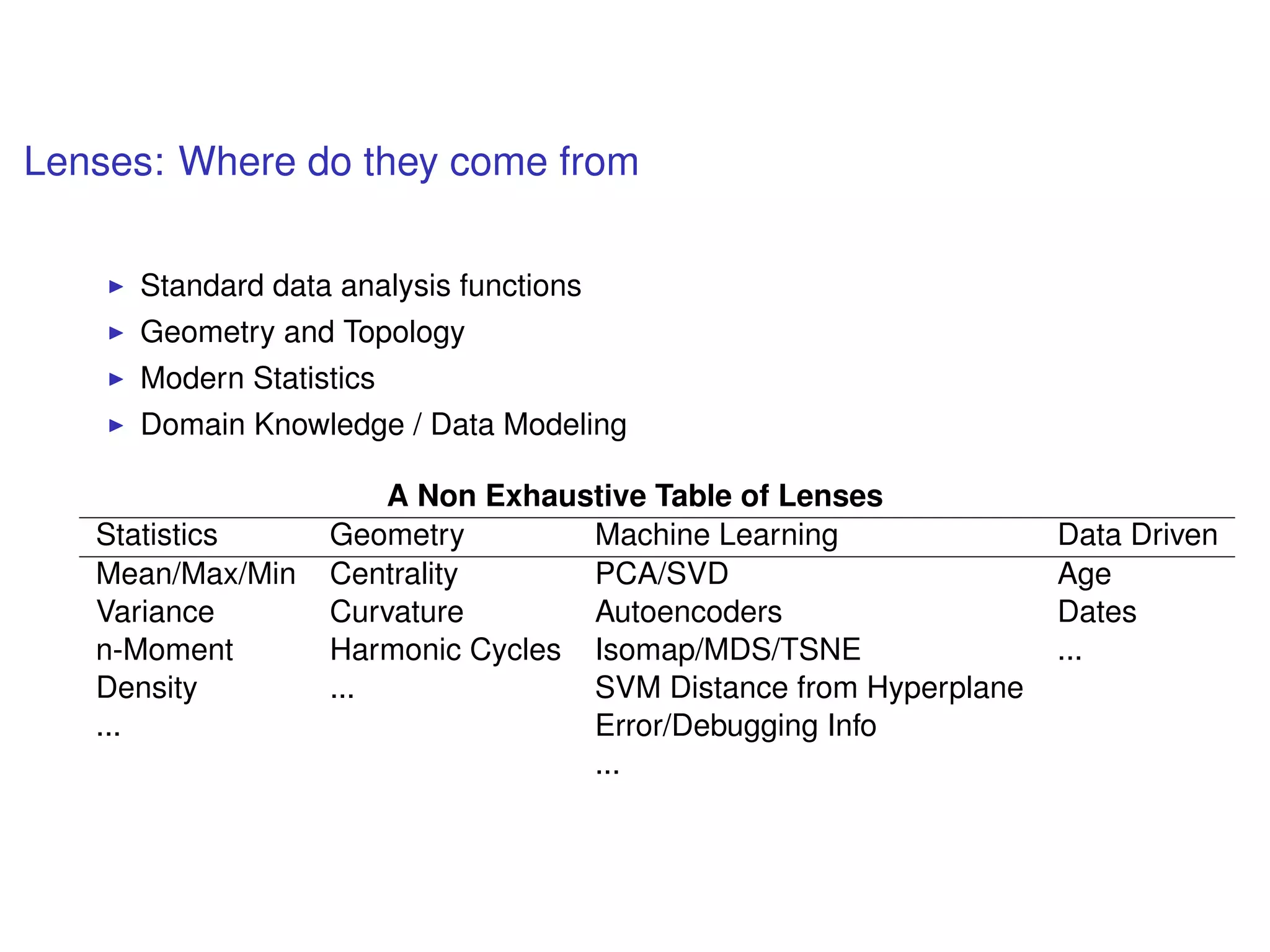
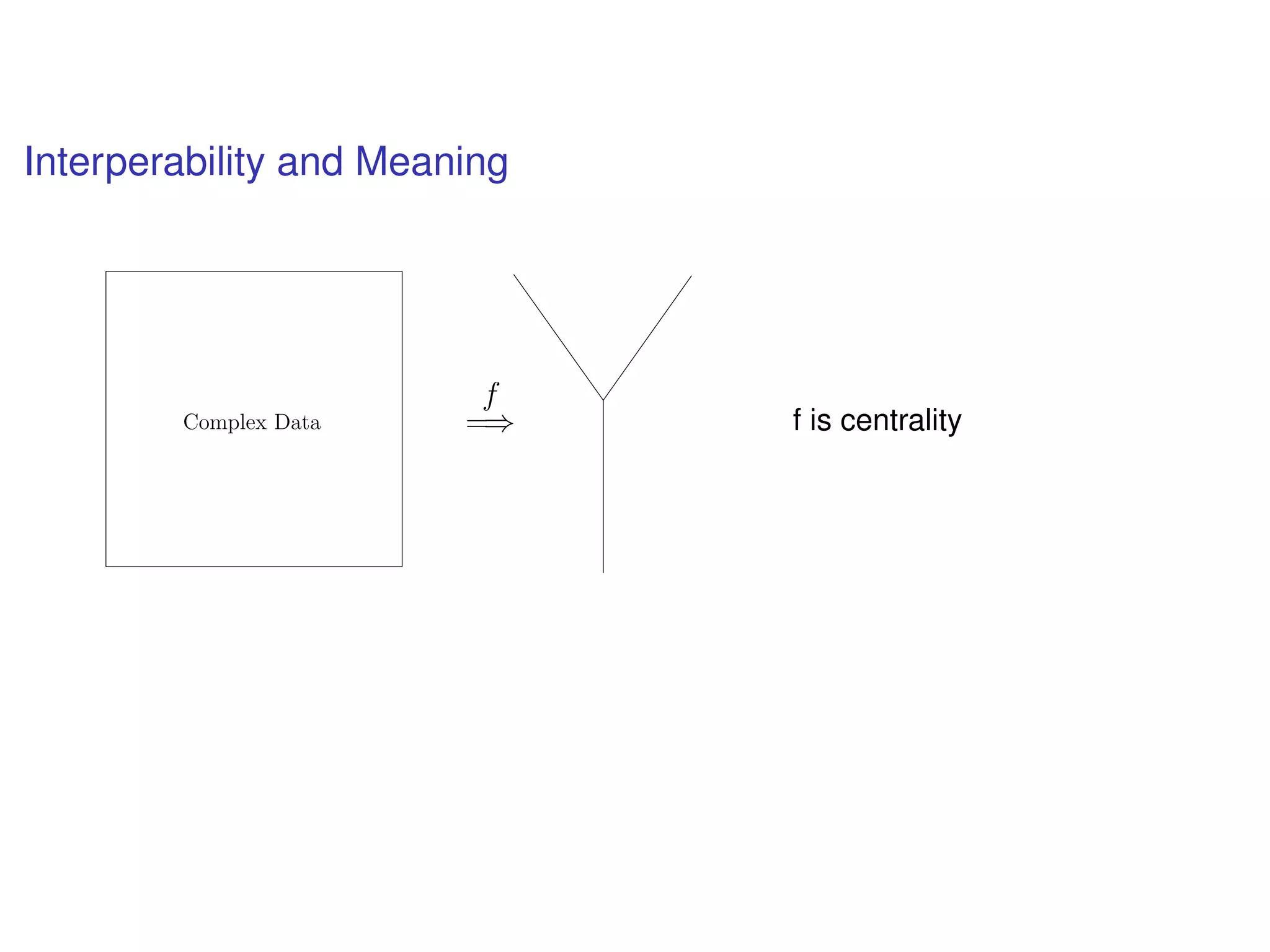
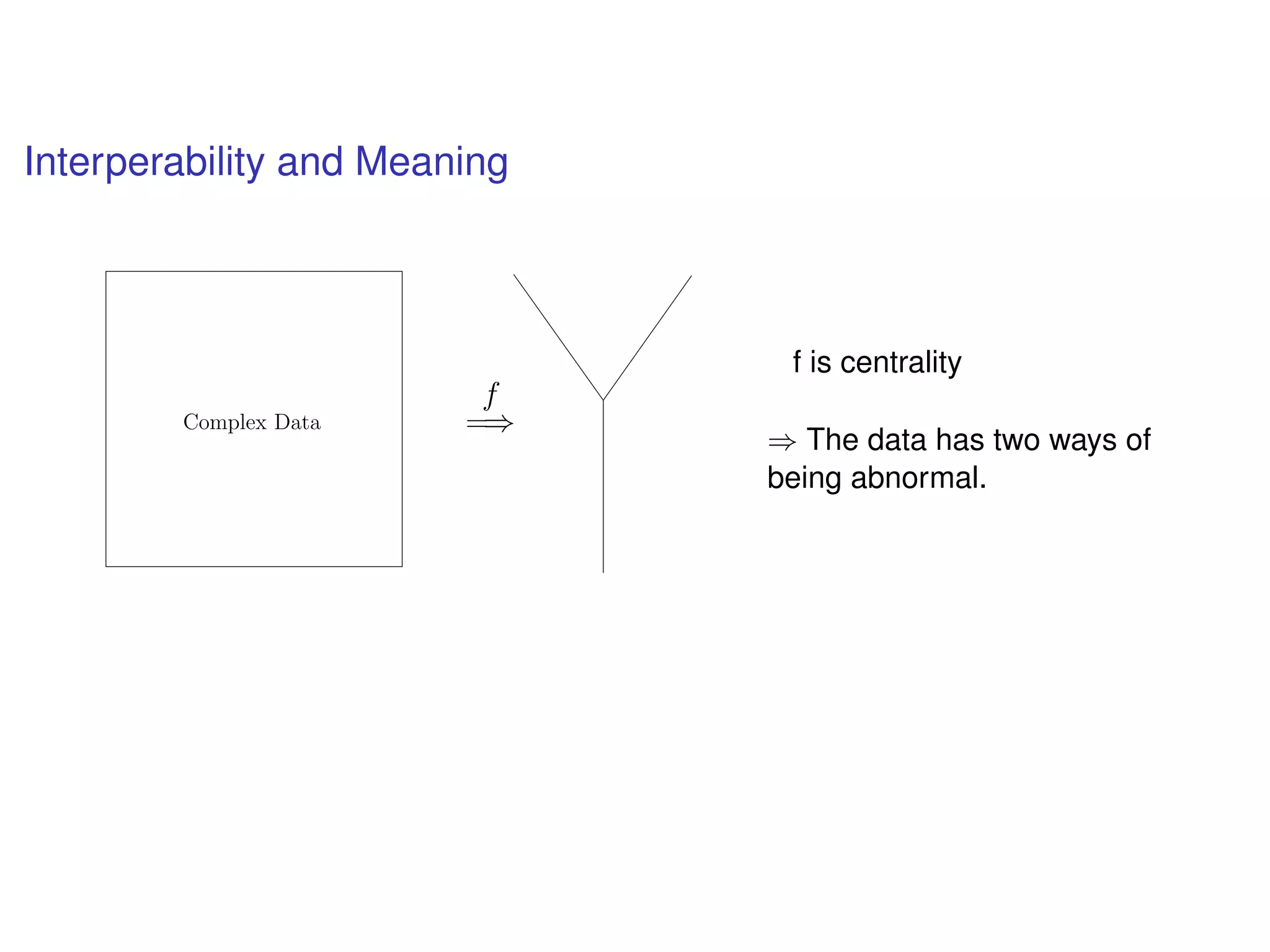
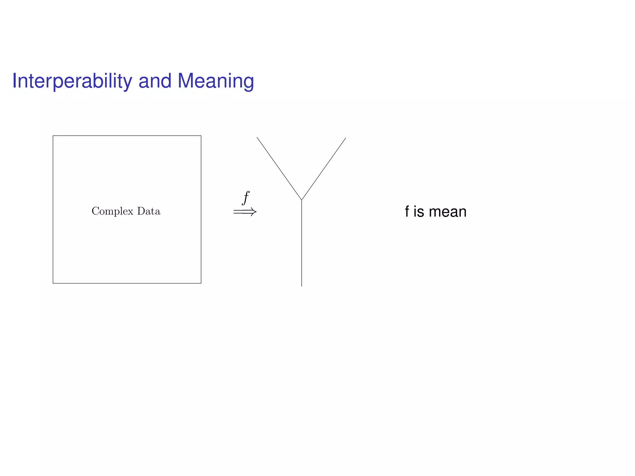
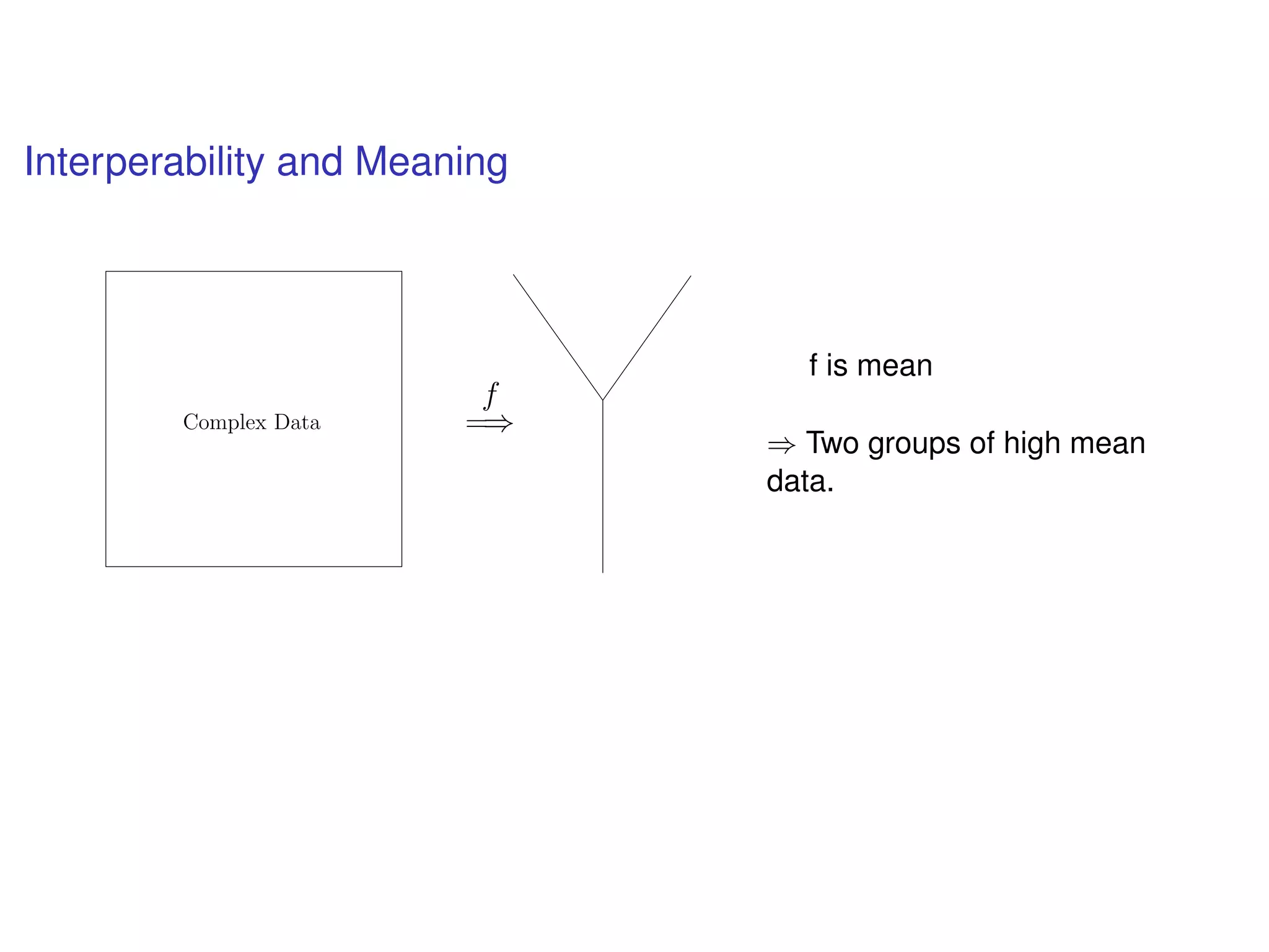
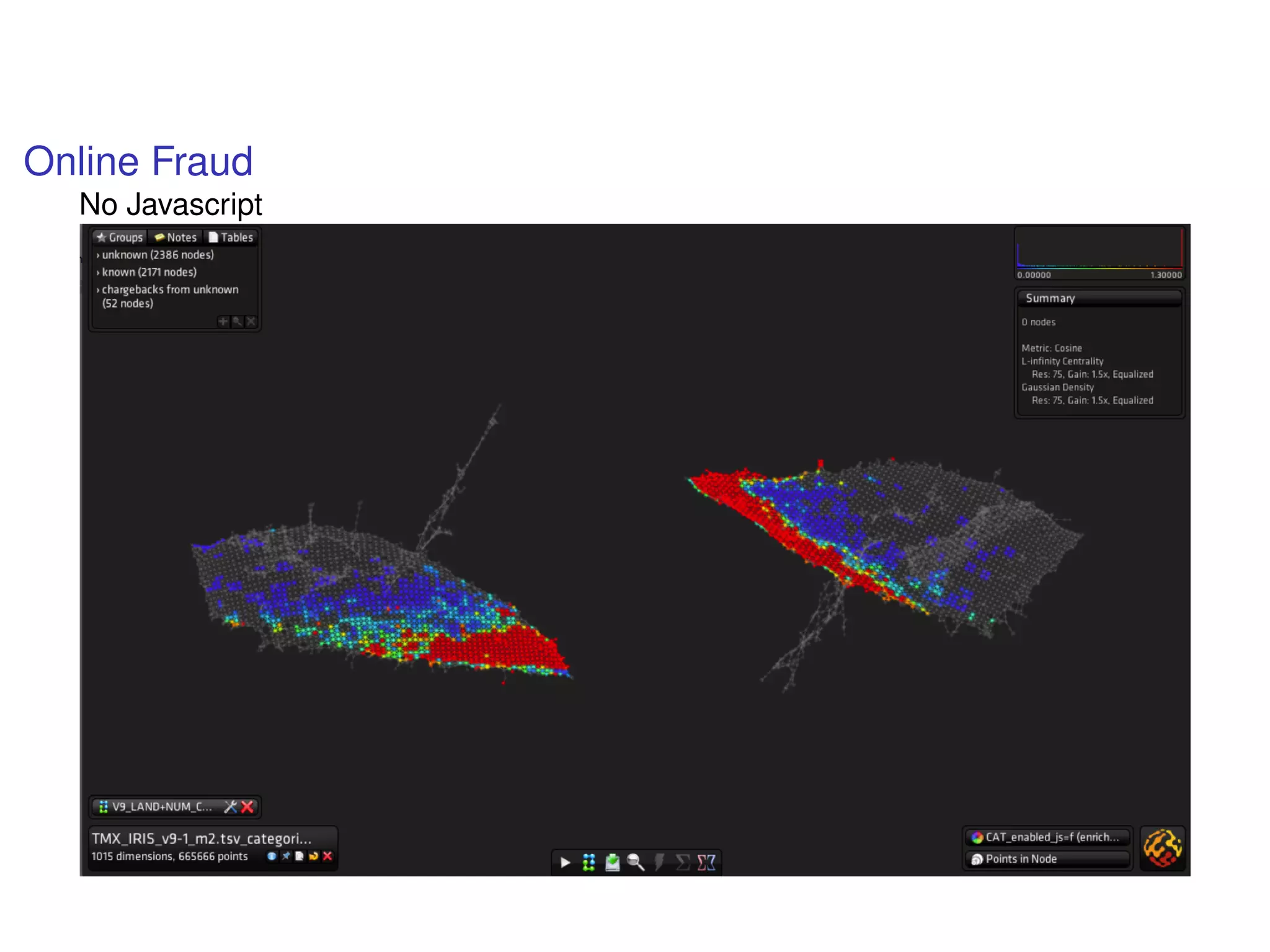
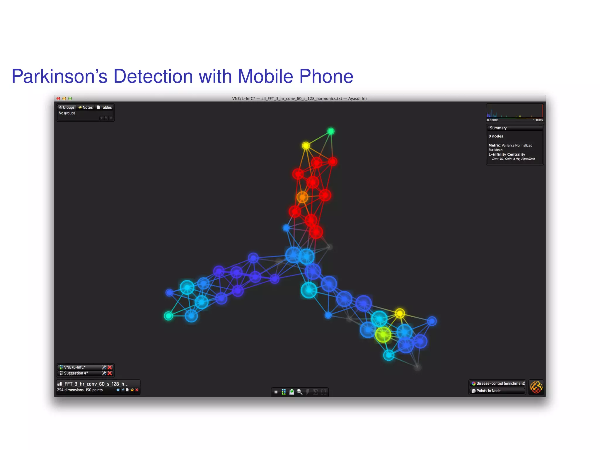
The document discusses topological data analysis (TDA) and its application in extracting meaningful insights from complex data, particularly through the Ayasdi framework. It outlines the challenges posed by big data and rich feature datasets, emphasizing that TDA can help summarize irrelevant data narratives to reveal significant patterns. The talk also explores methodologies and lenses used in TDA to visualize and analyze data effectively.

1. Shape and Meaning
An Introduction to Topological Data Analysis
Anthony Bak

2. Goals
For this talk I want to:

3. Goals
For this talk I want to:
Show you how TDA provides a framework for many machine learning/data
analysis techniques

4. Goals
For this talk I want to:
Show you how TDA provides a framework for many machine learning/data
analysis techniques
Demonstrate how Ayasdi provides insights into the data.

5. Goals
For this talk I want to:
Show you how TDA provides a framework for many machine learning/data
analysis techniques
Demonstrate how Ayasdi provides insights into the data.
Caveats: I am only talking about the strain of TDA done by Ayasdi

6. The Data Problem
How do we extract meaning from Complex Data?

7. The Data Problem
How do we extract meaning from Complex Data?
Data is complex because it’s "Big Data"

8. The Data Problem
How do we extract meaning from Complex Data?
Data is complex because it’s "Big Data"
Or has very rich features (eg. Genetic Data >500,000 features, complicated
interdependencies)

9. The Data Problem
How do we extract meaning from Complex Data?
Data is complex because it’s "Big Data"
Or has very rich features (eg. Genetic Data >500,000 features, complicated
interdependencies)
Or both!

10. The Data Problem
How do we extract meaning from Complex Data?
Data is complex because it’s "Big Data"
Or has very rich features (eg. Genetic Data >500,000 features, complicated
interdependencies)
Or both!
The Problem in both cases is that there isn’t a single story happening in your data.

11. The Data Problem
How do we extract meaning from Complex Data?
Data is complex because it’s "Big Data"
Or has very rich features (eg. Genetic Data >500,000 features, complicated
interdependencies)
Or both!
The Problem in both cases is that there isn’t a single story happening in your data.
TDA will be the tool that summarizes out the irrelevant stories to get at something
interesting.

12. Data Has Shape
And Shape Has Meaning

13. Data Has Shape
And Shape Has Meaning
⇒ In this talk I will focus on how we extract meaning.

14. But first... What is shape?

15. But first... What is shape?
Shape is the global realization of local constraints.

16. But first... What is shape?
Shape is the global realization of local constraints.
For a given problem determined by a choice of
Features, columns or properties to measure.
A metric on the columns.

17. But first... What is shape?
Shape is the global realization of local constraints.
For a given problem determined by a choice of
Features, columns or properties to measure.
A metric on the columns.
But not necessarily so. There are more relaxed definitions of shape and we
can use those too.

18. But first... What is shape?
Shape is the global realization of local constraints.
For a given problem determined by a choice of
Features, columns or properties to measure.
A metric on the columns.
But not necessarily so. There are more relaxed definitions of shape and we
can use those too.
The goal of TDA is to understand (for us, summarize) the shape with no
preconceived model of what it should be.

19. Math World
To show you how we extract insight from shape we start in "Math World"

20. Math World
To show you how we extract insight from shape we start in "Math World"
We’ll draw the data as a smooth manifold.

21. Math World
To show you how we extract insight from shape we start in "Math World"
We’ll draw the data as a smooth manifold.
Functions that appear are smooth or continuous.

22. Math World
To show you how we extract insight from shape we start in "Math World"
We’ll draw the data as a smooth manifold.
Functions that appear are smooth or continuous.
⇒ We will not need either of these assumptions once we’re in "Data World".

23. Math World
To show you how we extract insight from shape we start in "Math World"
We’ll draw the data as a smooth manifold.
Functions that appear are smooth or continuous.
⇒ We will not need either of these assumptions once we’re in "Data World".
⇒ Even more importantly, data in the real world is never like this

24. Math World
Data

25. Math World
f
p
Data

26. Math World
f
pf−1
(p)
Data

27. Math World
f
pf−1
(p)
=⇒
Data

28. Math World
f
pf−1
(p)
=⇒
q
Data

29. Math World
f
pf−1
(p)
=⇒
q
Data

30. Math World
f
pf−1
(p)
=⇒
q
Data

31. Math World
f
pf−1
(p)
=⇒
q
g
Data

32. Math World
f
pf−1
(p)
=⇒
q
g
Data
p

33. Math World
f
pf−1
(p)
=⇒
q
g
Data
p

34. Math World
f
pf−1
(p)
=⇒
q
g
Data
p q

35. Math World
f
pf−1
(p)
=⇒
q
g
Data
p q

36. Math World
f
pf−1
(p)
=⇒
q
g
Data
r

37. Math World
f
pf−1
(p)
=⇒
q
g
Data
r

38. Math World
f
pf−1
(p)
=⇒
q
g
Data

39. Exercise:
What is the summary if we use both lenses, g and f at the same time?
(g, f)

40. Exercise:
What is the summary if we use both lenses, g and f at the same time?
(g, f)

41. Exercise:
What is the summary if we use both lenses, g and f at the same time?
(g, f)
p

42. Exercise:
What is the summary if we use both lenses, g and f at the same time?
(g, f)
p

43. Exercise:
What is the summary if we use both lenses, g and f at the same time?
(g, f)
p

44. Exercise:
What is the summary if we use both lenses, g and f at the same time?
(g, f)
p

45. Exercise:
What is the summary if we use both lenses, g and f at the same time?
(g, f)
p
=⇒ We recover the original space

46. What did the exercise tell us?

47. What did the exercise tell us?
With a rich enough set of functions (lenses) we can recover the original space

48. What did the exercise tell us?
With a rich enough set of functions (lenses) we can recover the original space
Of course this leaves us no better off then where we started.

49. What did the exercise tell us?
With a rich enough set of functions (lenses) we can recover the original space
Of course this leaves us no better off then where we started.
⇒ Instead we select a set of functions to tune in to the signal we want.

50. This is what Ayasdi does:
f
pf−1
(p)
=⇒
q
g
Data

51. This is what Ayasdi does:
f
pf−1
(p)
=⇒
q
g
Data
Modulo some details....

52. Why is this useful?

53. Why is this useful?
⇒ We get "easy" understanding of the localizations of quantities of interest.

54. Why is this useful?
f
g

55. Why is this useful?
f
g

56. Why is this useful?
f
g

57. Why is this useful?
f
g

58. Why is this useful?
f
g

59. Why is this useful?
f
g

60. Why is this useful?
f
g

61. Why is this useful?
f
g

62. Why is this useful?
f
g

63. Why is this useful?

64. Why is this useful?
Lenses inform us where in the space to look for phenomena.

65. Why is this useful?
Lenses inform us where in the space to look for phenomena.
For easy localizations many different lenses will be informative.

66. Why is this useful?
Lenses inform us where in the space to look for phenomena.
For easy localizations many different lenses will be informative.
For hard ( = geometrically distributed) localizations we have to be more
careful.

67. Why is this useful?
Lenses inform us where in the space to look for phenomena.
For easy localizations many different lenses will be informative.
For hard ( = geometrically distributed) localizations we have to be more
careful. But even then, we frequently get incremental knowledge even from a
poorly chosen lens.

68. Modulo Details....
We want to move from this mathematical model to a data driven setup.

69. Step 1
f

70. Step 1
Replace points in the range with an open covering of the range.
f
((()))
U1
U2
U3

71. Step 1
Replace points in the range with an open covering of the range.
f
((()))
U1
U2
U3

72. Step 1
Replace points in the range with an open covering of the range.
f
((()))
U1
U2
U3

73. Step 1
Replace points in the range with an open covering of the range.
f
((()))
U1
U2
U3

74. Step 1
Replace points in the range with an open covering of the range.
f
((()))
U1
U2
U3

75. Step 1
Replace points in the range with an open covering of the range.
Connect nodes when their corresponding sets intersect.
f
((()))
U1
U2
U3

76. Step 1
Replace points in the range with an open covering of the range.
Connect nodes when their corresponding sets intersect.
f
((()))
U1
U2
U3

77. Step 1
Replace points in the range with an open covering of the range.
Connect nodes when their corresponding sets intersect.
f
((()))
U1
U2
U3
⇒ The output is now a graph.

78. New Parameters
We’ve introduced new parameters into the construction:

79. New Parameters
We’ve introduced new parameters into the construction:
The resolution is the number of open sets in the range.

80. New Parameters
We’ve introduced new parameters into the construction:
The resolution is the number of open sets in the range.
The gain is the amount of overlap of these intervals.

81. New Parameters
We’ve introduced new parameters into the construction:
The resolution is the number of open sets in the range.
The gain is the amount of overlap of these intervals.
Roughly speaking, the resolution controls the number of nodes in the output and
the ’size’ of feature you can pick out, while the gain controls the number of edges
and the ’tightness’ of the graph.

82. Resolution: A closer look
f
()()()()
U1
U2
U3
U4

83. Resolution: A closer look
f
()()()()
U1
U2
U3
U4

84. Resolution: A closer look
f
()()()()
U1
U2
U3
U4
()()

85. Resolution: A closer look
f
()()()()
U1
U2
U3
U4
()()

86. Step 2: Clustering as π0
We need to make a final adjustment to the algorithm to bring it into data world.

87. Step 2: Clustering as π0
We need to make a final adjustment to the algorithm to bring it into data world.
We replace "connected component of the inverse image" is with "clusters in
the inverse image".

88. Step 2: Clustering as π0
We need to make a final adjustment to the algorithm to bring it into data world.
We replace "connected component of the inverse image" is with "clusters in
the inverse image".
We connect clusters (nodes) with an edge if they share points in common.

89. Step 2: Clustering as π0
f

90. Step 2: Clustering as π0
f

91. Step 2: Clustering as π0
f
U1

92. Step 2: Clustering as π0
f
U1
U2

93. Step 2: Clustering as π0
f
U1
U2

94. Step 2: Clustering as π0
f
U1
U2

95. Step 2: Clustering as π0
f
U1
U2
Nodes are clusters of data points

96. Step 2: Clustering as π0
f
U1
U2
Nodes are clusters of data points
Edges represent shared points between the clusters

97. Step 2: Clustering as π0
f
U1
U2
Nodes are clusters of data points
Edges represent shared points between the clusters

98. Step 2: Clustering as π0
f
U1
U2
Nodes are clusters of data points
Edges represent shared points between the clusters

99. Step 2: Clustering as π0
f
U1
U2
Nodes are clusters of data points
Edges represent shared points between the clusters

100. Step 2: Clustering as π0
f
U1
U2
Nodes are clusters of data points
Edges represent shared points between the clusters

101. Step 2: Clustering as π0
f
U1
U2
Nodes are clusters of data points
Edges represent shared points between the clusters

102. Step 2: Clustering as π0
f
U1
U2
Nodes are clusters of data points
Edges represent shared points between the clusters

103. Step 2: Clustering as π0
f
U1
U2
Nodes are clusters of data points
Edges represent shared points between the clusters

104. Step 2: Clustering as π0
f
U1
U2
Nodes are clusters of data points
Edges represent shared points between the clusters

105. Step 2: Clustering as π0
f
U1
U2
Nodes are clusters of data points
Edges represent shared points between the clusters

106. Step 2: Clustering as π0
f
U1
U2
Nodes are clusters of data points
Edges represent shared points between the clusters

107. That’s It

108. That’s It
Ok not quite...

109. Lenses: Where do they come from
The technique rests on finding good lenses.

110. Lenses: Where do they come from
The technique rests on finding good lenses.
⇒ Luckily lots of people have worked on this problem

111. Lenses: Where do they come from
A Non Exhaustive Table of Lenses

112. Lenses: Where do they come from
Standard data analysis functions
A Non Exhaustive Table of Lenses
Statistics

113. Lenses: Where do they come from
Standard data analysis functions
A Non Exhaustive Table of Lenses
Statistics
Mean/Max/Min

114. Lenses: Where do they come from
Standard data analysis functions
A Non Exhaustive Table of Lenses
Statistics
Mean/Max/Min
Variance

115. Lenses: Where do they come from
Standard data analysis functions
A Non Exhaustive Table of Lenses
Statistics
Mean/Max/Min
Variance
n-Moment

116. Lenses: Where do they come from
Standard data analysis functions
A Non Exhaustive Table of Lenses
Statistics
Mean/Max/Min
Variance
n-Moment
Density

117. Lenses: Where do they come from
Standard data analysis functions
A Non Exhaustive Table of Lenses
Statistics
Mean/Max/Min
Variance
n-Moment
Density
...

118. Lenses: Where do they come from
Standard data analysis functions
Geometry and Topology
A Non Exhaustive Table of Lenses
Statistics Geometry
Mean/Max/Min
Variance
n-Moment
Density
...

119. Lenses: Where do they come from
Standard data analysis functions
Geometry and Topology
A Non Exhaustive Table of Lenses
Statistics Geometry
Mean/Max/Min Centrality
Variance
n-Moment
Density
...

120. Lenses: Where do they come from
Standard data analysis functions
Geometry and Topology
A Non Exhaustive Table of Lenses
Statistics Geometry
Mean/Max/Min Centrality
Variance Curvature
n-Moment
Density
...

121. Lenses: Where do they come from
Standard data analysis functions
Geometry and Topology
A Non Exhaustive Table of Lenses
Statistics Geometry
Mean/Max/Min Centrality
Variance Curvature
n-Moment Harmonic Cycles
Density
...

122. Lenses: Where do they come from
Standard data analysis functions
Geometry and Topology
A Non Exhaustive Table of Lenses
Statistics Geometry
Mean/Max/Min Centrality
Variance Curvature
n-Moment Harmonic Cycles
Density ...
...

123. Lenses: Where do they come from
Standard data analysis functions
Geometry and Topology
Modern Statistics
A Non Exhaustive Table of Lenses
Statistics Geometry Machine Learning
Mean/Max/Min Centrality
Variance Curvature
n-Moment Harmonic Cycles
Density ...
...

124. Lenses: Where do they come from
Standard data analysis functions
Geometry and Topology
Modern Statistics
A Non Exhaustive Table of Lenses
Statistics Geometry Machine Learning
Mean/Max/Min Centrality PCA/SVD
Variance Curvature
n-Moment Harmonic Cycles
Density ...
...

125. Lenses: Where do they come from
Standard data analysis functions
Geometry and Topology
Modern Statistics
A Non Exhaustive Table of Lenses
Statistics Geometry Machine Learning
Mean/Max/Min Centrality PCA/SVD
Variance Curvature Autoencoders
n-Moment Harmonic Cycles
Density ...
...

126. Lenses: Where do they come from
Standard data analysis functions
Geometry and Topology
Modern Statistics
A Non Exhaustive Table of Lenses
Statistics Geometry Machine Learning
Mean/Max/Min Centrality PCA/SVD
Variance Curvature Autoencoders
n-Moment Harmonic Cycles Isomap/MDS/TSNE
Density ...
...

127. Lenses: Where do they come from
Standard data analysis functions
Geometry and Topology
Modern Statistics
A Non Exhaustive Table of Lenses
Statistics Geometry Machine Learning
Mean/Max/Min Centrality PCA/SVD
Variance Curvature Autoencoders
n-Moment Harmonic Cycles Isomap/MDS/TSNE
Density ... SVM Distance from Hyperplane
...

128. Lenses: Where do they come from
Standard data analysis functions
Geometry and Topology
Modern Statistics
A Non Exhaustive Table of Lenses
Statistics Geometry Machine Learning
Mean/Max/Min Centrality PCA/SVD
Variance Curvature Autoencoders
n-Moment Harmonic Cycles Isomap/MDS/TSNE
Density ... SVM Distance from Hyperplane
... Error/Debugging Info

129. Lenses: Where do they come from
Standard data analysis functions
Geometry and Topology
Modern Statistics
A Non Exhaustive Table of Lenses
Statistics Geometry Machine Learning
Mean/Max/Min Centrality PCA/SVD
Variance Curvature Autoencoders
n-Moment Harmonic Cycles Isomap/MDS/TSNE
Density ... SVM Distance from Hyperplane
... Error/Debugging Info
...

130. Lenses: Where do they come from
Standard data analysis functions
Geometry and Topology
Modern Statistics
Domain Knowledge / Data Modeling
A Non Exhaustive Table of Lenses
Statistics Geometry Machine Learning Data Driven
Mean/Max/Min Centrality PCA/SVD
Variance Curvature Autoencoders
n-Moment Harmonic Cycles Isomap/MDS/TSNE
Density ... SVM Distance from Hyperplane
... Error/Debugging Info
...

131. Lenses: Where do they come from
Standard data analysis functions
Geometry and Topology
Modern Statistics
Domain Knowledge / Data Modeling
A Non Exhaustive Table of Lenses
Statistics Geometry Machine Learning Data Driven
Mean/Max/Min Centrality PCA/SVD Age
Variance Curvature Autoencoders
n-Moment Harmonic Cycles Isomap/MDS/TSNE
Density ... SVM Distance from Hyperplane
... Error/Debugging Info
...

132. Lenses: Where do they come from
Standard data analysis functions
Geometry and Topology
Modern Statistics
Domain Knowledge / Data Modeling
A Non Exhaustive Table of Lenses
Statistics Geometry Machine Learning Data Driven
Mean/Max/Min Centrality PCA/SVD Age
Variance Curvature Autoencoders Dates
n-Moment Harmonic Cycles Isomap/MDS/TSNE
Density ... SVM Distance from Hyperplane
... Error/Debugging Info
...

133. Lenses: Where do they come from
Standard data analysis functions
Geometry and Topology
Modern Statistics
Domain Knowledge / Data Modeling
A Non Exhaustive Table of Lenses
Statistics Geometry Machine Learning Data Driven
Mean/Max/Min Centrality PCA/SVD Age
Variance Curvature Autoencoders Dates
n-Moment Harmonic Cycles Isomap/MDS/TSNE ...
Density ... SVM Distance from Hyperplane
... Error/Debugging Info
...

134. Interperability and Meaning
But what about insight? meaning?

135. Interperability and Meaning
f
=⇒Complex Data

136. Interperability and Meaning
f
=⇒Complex Data f is gaussian density

137. Interperability and Meaning
f
=⇒Complex Data
f is gaussian density
⇒ The data is bi-modal.

138. Interperability and Meaning
f
=⇒Complex Data f is centrality

139. Interperability and Meaning
f
=⇒Complex Data
f is centrality
⇒ The data has two ways of
being abnormal.

140. Interperability and Meaning
f
=⇒Complex Data f is mean

141. Interperability and Meaning
f
=⇒Complex Data
f is mean
⇒ Two groups of high mean
data.

142. Interperability and Meaning
f
=⇒Complex Data f is error

143. Interperability and Meaning
f
=⇒Complex Data
f is error
⇒ Two types of error.

144. Interperability and Meaning
f
=⇒Complex Data
f is error
⇒ Two types of error.
The units on the lens give interperability/meaning to the topological summary.

145. Interperability and Meaning
Another way to think about lenses is as a kind of ’geometric query’.
Examples

146. Interperability and Meaning
Another way to think about lenses is as a kind of ’geometric query’.
Examples
1. Heart disease study

147. Interperability and Meaning
Another way to think about lenses is as a kind of ’geometric query’.
Examples
1. Heart disease study
Stratification by age without making arbitrary cutoffs.

148. Interperability and Meaning
Another way to think about lenses is as a kind of ’geometric query’.
Examples
1. Heart disease study
Stratification by age without making arbitrary cutoffs.
2. Heavy machinery

149. Interperability and Meaning
Another way to think about lenses is as a kind of ’geometric query’.
Examples
1. Heart disease study
Stratification by age without making arbitrary cutoffs.
2. Heavy machinery
Use mean a variance as a lens to find what operating regimes lead to failure of
mechanical components.

150. Some generalizations and extensions

151. Some generalizations and extensions
Metrics

152. Some generalizations and extensions
Metrics
We don’t need a metric, just a notion of similarity - or perhaps a clustering
mechanism.

153. Some generalizations and extensions
Metrics
We don’t need a metric, just a notion of similarity - or perhaps a clustering
mechanism.
Lenses

154. Some generalizations and extensions
Metrics
We don’t need a metric, just a notion of similarity - or perhaps a clustering
mechanism.
Lenses
Lenses don’t need to be continuous - just "sensible".

155. Some generalizations and extensions
Metrics
We don’t need a metric, just a notion of similarity - or perhaps a clustering
mechanism.
Lenses
Lenses don’t need to be continuous - just "sensible".
We can use multiple lenses at the same time.

156. Some generalizations and extensions
Metrics
We don’t need a metric, just a notion of similarity - or perhaps a clustering
mechanism.
Lenses
Lenses don’t need to be continuous - just "sensible".
We can use multiple lenses at the same time.
Lenses can map to space other then R.

157. Some generalizations and extensions
Metrics
We don’t need a metric, just a notion of similarity - or perhaps a clustering
mechanism.
Lenses
Lenses don’t need to be continuous - just "sensible".
We can use multiple lenses at the same time.
Lenses can map to space other then R.
In fact, can work with "open covers" of the space (Here taken to mean
overlapping partitions). Don’t need a lens at all.

158. Some generalizations and extensions
Metrics
We don’t need a metric, just a notion of similarity - or perhaps a clustering
mechanism.
Lenses
Lenses don’t need to be continuous - just "sensible".
We can use multiple lenses at the same time.
Lenses can map to space other then R.
In fact, can work with "open covers" of the space (Here taken to mean
overlapping partitions). Don’t need a lens at all.
Data

159. Some generalizations and extensions
Metrics
We don’t need a metric, just a notion of similarity - or perhaps a clustering
mechanism.
Lenses
Lenses don’t need to be continuous - just "sensible".
We can use multiple lenses at the same time.
Lenses can map to space other then R.
In fact, can work with "open covers" of the space (Here taken to mean
overlapping partitions). Don’t need a lens at all.
Data
Input space can be anything with a topology. Typically we work with
row/column numeric/categorical data but, for example, graphs are ok.

160. Some generalizations and extensions
Metrics
We don’t need a metric, just a notion of similarity - or perhaps a clustering
mechanism.
Lenses
Lenses don’t need to be continuous - just "sensible".
We can use multiple lenses at the same time.
Lenses can map to space other then R.
In fact, can work with "open covers" of the space (Here taken to mean
overlapping partitions). Don’t need a lens at all.
Data
Input space can be anything with a topology. Typically we work with
row/column numeric/categorical data but, for example, graphs are ok.
Output

161. Some generalizations and extensions
Metrics
We don’t need a metric, just a notion of similarity - or perhaps a clustering
mechanism.
Lenses
Lenses don’t need to be continuous - just "sensible".
We can use multiple lenses at the same time.
Lenses can map to space other then R.
In fact, can work with "open covers" of the space (Here taken to mean
overlapping partitions). Don’t need a lens at all.
Data
Input space can be anything with a topology. Typically we work with
row/column numeric/categorical data but, for example, graphs are ok.
Output
The output of the algorithm isn’t just a graph but is an abstract simplicial
complex (swept under the rug in this presentation).

162. Demo

163. Online Fraud
Fraud Score

164. Online Fraud
Charge Back (Ground Truth)

165. Online Fraud
Time On Page

166. Online Fraud
No Flash

167. Online Fraud
No Javascript

168. Parkinson’s Detection with Mobile Phone