Putra Business School GSM5421 Investment Analysis MBA Quick Notes

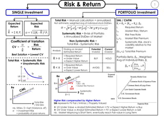
1. 1Risk & Return
PORTFOLIO Investment
Expected
Return
= Σ Ri Pi
^
R σ = √ Σ(Ri - R )2.Pi
Expected
Risk
^
SINGLE Investment
Analysis
Finding on Analyst
Estimated Return
Potential
Investor
Current
Investor
Ȓ > R
> Required Return
⇒ Under Value
⇒ Expect Higher Return
BUY HOLD
Ȓ < R
< Required Return
⇒ Over Value
⇒ Expect Lower Return
AVOID SELL
CV = =
σ
^
R
Risk
Return
Coefficient of Variation
Best Solution = Lowest CV
Invi
Invtot
βP = Σ x Pi
SML / CAPM
Ri = Rrf + (Rm – Rrf). βP
ri Required Return
rm Market Risk / Return
rrf Risk Free Rate
rm-rrf Market Risk Premium
β Systematic Risk, stock’s
volatility relative to the
market
β(rm-rrf) Total Risk Premium
Portfolio Beta, βP = Weighted
Avg of Individual Risks, βi
UR = DR
SR = MR
SML
Higher Risk compensated by Higher Return
SM represents FV Fair / Intrinsic / Properly Valued
 UV Under Value ⇒ Analyst Estimated Return > FV ⇒ Expect Higher Return ⇒ Buy
 OV Over Value ⇒ Analyst Estimated Return < FV ⇒ Expect Lower Return ⇒ Sell
nb. Market Mispricing is Short Term, eventually reach Fair-value in Long Term
Rf
σ
Re
Total Risk
/ Std Dev
nb. StDev, ŝ = Sqrt (Variance, σ2)
σ = Investment Risk
= probability of poor returns
Rm
Rf
β
Re
β = 1
UV
OV
FV
Systematic
Risk
Slope
= (Rm – Rf)
= Market Risk Premium
Total Risk = Systematic Risk
+ Unsystematic Risk
Total Risk = Manual calculation + annualized;
Not arithmetic weighted avg of individual stock StdDev.
Systematic Risk = Β-risk of Portfolio
x Annualized StdDev of Market
Non-Systematic Risk =
Total Risk - Systematic Risk

2. Interest
Rate Risk
Purchasing
Power Risk
Business /
Liquidity Risk
Financial /
Credit Risk
Operational
Risk
Systematic Risk (Macro)
▌ @ Non-diversifiable Risk, Undiversifiable Risk, Market
Risk, Economic Risk, Volatility, Beta Risk
▌ Inherent and associated to entire market,
not just a particular stock or industry
▌ Underlies all other investment risks
▌ Impossible to mitigate by Portfolio Diversification
▌ Reduce exposure through hedging
▌ Higher Undiversifiable Risk
rewarded by Higher Return
▌ Beta = volatility compared to overall market
 > 1 means more systematic risk than the market
 < 1 means less systematic risk than the market
 = 1 means the same systematic risk as the market
Unsystematic Risk (Micro)
2
▌ @ Non-systematic Risk, Unsystematic Risk,
Diversifiable Risk, Company Specific Risk, Portfolio
Risk, Residual Risk
▌ Very broad group or individual securities, as stocks
of particular jurisdiction tend to move together
▌ Mitigation through Diversification – mix / different
companies, industries, uncorrelated assets,
securities, time frame, required rate of return and
risk tolerance
Total Risk
Absolute Relative
Directional
Non
Directional
Volatility
Exchange
Rate
GDP
Industrial
Growth
Price
Reinvestme
nt Rate
Political
Governme
nt Policies
Scams
War Like
Situation
Monsoon
Natural
Calamities
Internation
al Events
Demand
Inflation
Cost
Inflation
Internal External
Cash Flow Default
Portfolio
Exposure
Rate
Recovery
Rate
Credit
Event
Sovereign
Settlement Borrowings
Model People
LegalRecession
New
Competitor
Product
Recall
Policy
Political
Political
Market
Risk

3. 3
Non-Fixed Income: Stocks
rs = rrf + (rm – rrf). β
rs Required Rate of Return
rrf Risk Free Rate
β Beta Risk
rm Mkt Risk
rm – rrf Mkt Risk Premium
β(rm – rrf) Risk Premium
Dn Dividend in Yr n
g Growth Rate
Dividend Yield = Dn+1/Pn
Price, Pn+1 = Pn (1+gn)
Dividend, Dn+1 = Dn (1+gn)
Multiple / Supernormal Growth
Dividend & Capital Gains Yld not constant. Capital Gains Yld ≠ g.
1. Tabulate FCF = NOPAT – Net Capital Investment
2. TV = Stock Price when dividend growth constant
3. NPV = ΣPV(Future Div + FCFs - Debts - PrefShrs) - InitOutlay
4. Market Value (MV) = NPV / NOSH (common stock)
Relative Valuation
• Price to Earning (P/E)
• Price to Sales (P/S)
• Price to Cash Flow (P/CF)
• Price to Book Value (P/BV)
• Enterprise Val to EBITDA (EV/EBITDA)
• Enterprise Val to Revenue (EV/Revenue)
Discounted Cash Flow / Present Value
Best Method – Represent Expected Cashflows & Arbitrages.
Problem: Intrinsic value subject to quality of forecast.
Value of Returns = PV of future benefits
= PV of Dividends + Free Cash Flow (e.g. Capital Gains)
Intrinsic Value = Fair / Expected Value
FA Indicator IV > MP  Under-Priced
IV = MP  Fairly Valued
IV < MP  Over-Priced
Asset Based / Book Value
Useful when firm has high tangible assets + liabilities,
or low proportion intangible assets,
or deteriorating business (worst-case).
1.Statement of Comp Income / Balance Sheet
2.Book Value of assets and liabilities
3.Value of additive parts
4.MV(Equity) = MV(Assets+Liabilities–PrefShares)
5.Divide by NOSH
Problem:
1. Difficult to determine MV of Asset (PPE)
2. Intangibles not on balance sheet,
e.g. IP, synergies, reputation
3. If intangibles significant, use floor value or fwd CF
4. Difficult to estimate in hyper-inflation environment
=
(1 + )
Dividend Discount
Model (DDM)
Present Value of all future
dividends generated
=
(1 + )
Corporate Value Model
or Free Cash Flow (FCF)
or Operating Cash Flow
Subject to growth rate.
Constant Growth
g constant forever
rs > g
=
−
=
(1 + )
−
Zero Growth
Dividend is
Perpetual, g=0
=
Multiplier:
Estimate based on multiples of share price or
enterprise value to certain comparable value
or fundamental value, e.g. earnings, EBITDA,
book value, sales, cashflow. EV = Total Market
Capitalization plus Liabilities plus Preferential
Shares less Cash and equivalents.
• Fwd basis, e.g. EPS forecast for next year
• Trailing basis, e.g. EPS for past year
• Must be consistent across companies
Favorite price multiples include:
• Price-to-Earnings ratio (P/E) most
frequently cited, or to EBITDA
• Price-to-Book ratio (P/B)
• Price-to-Sales ratio (P/S)
• Price-to-Cashflow ratio (P/CF), i.e. free
cashflow (FCF), operating cash flow (OCF)
Price multiples is then analyzed using DCF
method, e.g. Gordon growth model.
Comparable:
Based on relative values of price multiples,
which is the most widely used approach by
analysts; both cross-sectional (versus the
market or another comparable) and in time
series. Approach easy to calculate and
beneficial for particular industry / sector,
which need to identify the best performing
stocks within sector. Large firms operate
different lines of business, scale and scope.
Problem: Choice of comparable. Price and
enterprise ratios do not consider the future.
CF1 CF2 CF3 CF4
Growth g1 g2 G3 gt
Dividend D1 D2 = D1(1+g) D3 = D1(1+g) D4 = D3
Price , =
−
NPV
(1 + ) (1 + ) (1 + )
+
(1 + )
Yr1 Yr2 Yr3 Yr4 to forever
Terminal Value

4. Intrinsic Value = Fair / Expected Value
FA Indicator IV > MP  Under-Valued
IV = MP  Fairly Valued
IV < MP  Over-Valued
Terminal Value
Super Normal Growth
Dividend & Cap Gains Yld not constant. Cap Gains Yld ≠ g.
1. Company Strategic Analysis
2. Establish Key Assumptions / Strategy
3. Tabulate FCF = NOPAT – Net Capital Investment
4. TV = Stock Price when dividend growth constant
5. NPV = ΣPV(FutDiv + FCFs - Debts - PrefShrs) - InitOutlay
6. Market Value (MV) = NPV / NOSH (common stock)
Yr1 Yr2 Yr3 Yr4 to forever
4
Non-Fixed Income: Stocks
rs = rrf + (rm – rrf). Β Growth, g Price, Pn+1 = Pn (1+gn)
Div Yield = Dn+1/Pn Div, Dn+1 = Dn (1+gn)
4. Precedent Transactions
1. Define M&A transaction same profile
• Business activity, geo-location, transaction
/ buyer, scale, growth, recent time period
2. Find Past Transactions
• Price paid
• Consideration (cash / shares)
• Takeover premium (implied or explicit)
• Synergies (if available)
• Other terms / conditions
3. Build Table & Ratios at transaction time
4. Calc Avg Multiples (Median if outliers)
5. Work backward towards EV
• Earning, EBITDA, EBIT, Sales, CF, CE, BV
2. Discounted Cash Flow / Present Value
Best Method = Represent Expected Cashflows & Arbitrages.
Problem: Intrinsic value subject to quality of forecast.
Value of Returns = PV of future benefits
= PV of Dividends + Free Cash Flow (e.g. Capital Gains) 1. Book Value / Asset-Based
Useful when firm has high tangible assets + liabilities,
or low proportion intangible assets,
or deteriorating business (worst-case).
1.Statement of Comprehensive Income
or Balance Sheet
2.Book Value of assets & liabilities
3.Value of additive parts
4.Equity = Assets – Liabilities – PrefShares; or
Equity = Share Capital – Treasury Shares +
Retained Earnings + Other Stockholder Equity
5.Divide by NOSH
Problem:
1. Difficult to determine MV of Asset (PPE)
2. Intangibles not on balance sheet,
e.g. IP, synergies, reputation
3. If intangibles significant, use floor value or fwd CF
4. Difficult to estimate in hyper-inflation environment
=
(1 + )
Dividend Discount
Model (DDM)
Present Value of all future
dividends generated
=
(1 + )
Corporate Value Model
or Free Cash Flow (FCF)
or Operating Cash Flow
Subject to growth rate.
Constant Growth
g constant forever, rs > g
=
−
=
(1 + )
−
Zero Growth
Dividend is Perpetual, g=0
=
CF1 CF2 CF3 CF4
Growth g1 g2 G3 gt
Div D1 D2 = D1(1+g) D3 = D1(1+g) D4 = D3
Price , =
−
NPV
(1 + ) (1 + ) (1 + )
+
(1 + )
3. Comparable / Relative Value
1. Select COMPS Universe / Peers same profile
• Industry, activity, geo-location, scale, growth,
profitability, acc’ policies, capital structure
2. Download Historical / Trailing Data
• Revenue, GrossProfit, EBITDA, EBIT, NPAT
• NOSH, SharePrices, Cash, Debt, Minority interest
3. Download Forecast Metrics
• Revenue, Gross profit, EBTIDA, EBIT, net income
4. Build Forward Table
• MarketCap, EV, Ratios, Growth, Margins, etc
5. Calc Average Multiples (Median if outliers)
 Enterprise Value Ratio (Before Interest Paid)
– EV to EBITDA
(Common for DCF analysis = core revenue)
– EV to EBIT
– EV to Revenue = EV/EBIT x EBIT/Sales
– EV to CE = EV/(BVDebt+Equity)
 Equity Value Ratio (After Interest Paid)
– Price to Earning (P/E) = MC/NetEarnings
– Price to Book Value = MC/BookValue
– Price to Cash Flow
6. Work backward towards Market Cap or EV
• Earning, EBITDA, EBIT, Sales, CF, CE, BV
Multiple Characteristics Stage
EV /Sales • No cash or profit
• Pattern of sales clear
• Ignores operating
economics
• Ignores capital structure
• Early sign
growth
• Rapid growth
EV/EBITDA • Operating cash flow
positive
• Incorporates profitability
• Ignores capital structure
• Ignores tax differences
• Rapid growth
• Slowing
growth
EV/EBIT • Operating profit
• Ignores capital structure
• Ignores tax differences
• Slowing
growth
• Maturity
P/E • Stable operating
economics
• Stable capital structure
• Profit & cash flow similar
• Early maturity
• Late maturity
Gross Profit = Revenue - Variable Cost
EBITDA = Gross Profit - Fixed Cost
EBIT = Oper Profit = EBITDA - NonCash
EBT = EBIT - Cost of Debt
NOPAT = EBT (1-Tax)
OCF = NOPAT + NonCash ± ∆WorkgCap
FCF = OCF (PreInvest CF) + CAPEX
EV = MarketCap + NetDebt
Net Debt = Interest Bearing Debt – Cash Eqv

5. Valuation Metrics Lions Gate Trading Precedents Warner**
EV/EBITDA* 13.7x / 11.4x 7.4x – 18.1x 8.3x – 27.6x 10.1x
EV/Sales* 1.8x / 1.7x 1.8x – 3.6x 1.2x – 5.3x 2.7x
P/E* 27.1x / 18.9x 13.3x – 40.9x 21.2x 17.1x
EBITDA Margin 9.5% 23% – 30% 3% – 55% 23.2%
Net Income Margin 8.5% 8% – 15% 26% 12.7%
5Sample Valuation Summary
Broker Estimates (M/D/Y) Results Period Revenues ($mm) EBITDA($mm) EBITDA Margin (%) EV/EBITDA P/E
RBC (11/18/2013)
Target Price $38.00 2014E 2,791 359 12.9% NA NA
EV ($mm) NA 2015E 2,887 407 14.1% NA 26.1x
J.P. Morgan (05/31/2013)
Target Price $32.00 2014E 2,651 345 13.0% 13.9x 24.7x
EV ($mm) $4,795 2015E 2,851 408 14.3% 11.8x 18.2x
Evercore (11/10/2013)
Target Price $42.00 2014E 2,877 375 13.0% 13.2x 30.7x
EV ($mm) $4,945 2015E 3,049 471 15.4% 10.5x 20.2x
0
200
400
600
800
1000
1200
1400
1600
1800
2000
$0
$5
$10
$15
$20
$25
$30
$35
$40
LGF
Current: $31.64 52wk High: $15.26 52wk Low: $37.81
*P/E and EV/EBITDA are based on FY14 and FY15 to reflect imminent growth; **based on FY14
 GUY appears to be valued fairly relative to peer group but peer group valuation has
come down recently
 Current Price low relative to Two-Year Trading Range due to recent drop in sector
and overall market index
 One-year Analyst forecasts are optimistic due to:
– Expected de-risking of asset priced into target
– Expected resource update (Q1 2012)
 There may be benefit to further de-risking as current valuation may not be optimal
time to sell
 Stock has outperformed based on strong cashflows from Twilight and Hunger
Games in 2012
 Current multiples are high but compress in FY14 / FY15 as growth is realized
 Industry multiples support share price but only if Hunger Games meets its forecast
 Further upside could be possible if another hit is produced but downside risk is more
significant
 Lions Gate produced limited or no free CF in 2007-2011 despite big successes
Football Field Analysis
Factors to Stock Price Performance

6. Proposition Weak form EMH Semi-strong form EMH Strong form EMH
Market is
Efficient
 Efficiently priced wrt
historical info
⸫ Exploit public info using FA
 Efficiently priced wrt
historical & public info
⸫ Exploit private / insider info
 Efficiently priced wrt to
historical, public & insider info
⸫ Cannot consistently beat mkt
Market is
NOT Efficient
 Inefficiently priced wrt
historical info
 Exploit by BF
 Inefficiently priced wrt
historical info
 Exploit by BF
 Inefficiently priced wrt
historical info
 Exploit by BF
6Efficient Market Hypothesis (EMH)
Fama (1969) States that mkt tend to be correctly & efficiently priced. Most mkts including Malaysia, US, China, Singapore
are in the Semi-Strong Form. Under developed countries exist in the Weak Form. No country in Strong Form.
 Fundamental Analysis (FA) = Fair Value or Intrinsic Value Indicator
 Technical Analysis (TA) = Buy / Hold / Sell or Entry / Exit Signal
 Behavioral Finance (BF) = Market Sentiments / Speculation
Speculators and traders still make money from small + short term mispricing opportunities, due to:
 Different method for stock valuation (DCF, comparable, dividend)
 Different source of information
 Different frequency
 Market delays / response
However, FA & TA & BF is an art & not science  Paralysis of Analysis = Complicated Decision
Historical Analysis Scenario Analysis
Return
RA = (SR)/n = AVERAGE
RG = [P(Return Relatives)]1/n – 1 = GR
E(R) = S Pi Ri
Risk
s2 = [S(Rt-RA)2]/n-1
s = √{[S(Rt-RA)2]/n-1} = STDEV
s2 = SPi[Ri-E(R)]2
s= √ {SPi[Ri-E(R)]2}
CV CV = s/RA CV = s/E(R)
Pot Return Rpot= w1 R1 + w2 R2 E(Rpot) = w1 R1 + w2 R2
Pot Risk
σpot
2 = w1
2σ1
2 + w2
2σ2
2 + 2W1W2 Cov(r1r2)
σpot
2 = w1
2σ1
2 + w2
2σ2
2 + 2W1W2 Correl(1,2)*σ1σ2-VARp
σpot = √σpot
2
(STDEVp)
σpot
2 = w1
2σ1
2 + w2
2σ2
2 + 2W1W2 Cov(r1r2)
σpot = √σpot
2
Arithmetic Mean = Simple avg of series of returns. Calculated by summing all of returns in the series and dividing by the number of values.
Geometric Mean = Return that if earned in each of n years of an investment’s life, gives same total dollar result as the actual investment.

7. Fixed Income: Bonds 7
N = Maturity Period / Duration
@ Years to Maturity x Compounding (M)
i.e. 1 yearly, 2 semi annual, 4 quarterly
I/YR = YTM = Interest on Bond
@ FV RM1000 to PV at I/YR
PV = Present Value
@ Price of Bond Sold / Purchased
Inc. Floatation Cost at PVf = PV0 (1-FC)
PMT = Coupon Payment
or Cashflow at ROR or Promised Yield
@ Coupon Rate x RM1000
FV = Par / Face Value
Principal @ Redeem at Maturity i.e. RM1K
CY = Current Yield
= Annual PMT / (PV or Current Price)
CGY = Capital Gains Yield
= P1/P0 - 1
= Total Yield – Current Yield
Expected Total Return
= Expected CY + Expected CGY
1. Fixed Term & Coupon Rate
2. Floating Rate periodically review
3. Zero coupon
4. Inflation Linked
5. Callable
6. Convertible
Factors affecting Bond, R = Rfr + Rinf + Rprem
• Macro Economic Factors: Real Growth, Expected Inflation,
Capital Market Liquidity, Supply / Demand Loans
• Bond Characteristics: Bond Rating / Credit Quality,
Terms to Maturity, Indenture Provision, Foreign Bond Risk
• Coupon Rate: inverse var to sensitivity
• Effective Maturity: Maturity & Duration: direct var to sensitivity
YTC
 PMT & FV = same
 PV1 = PV0 + (Penalty RM or %)
 n = Reduced by lapsed Years
 YTC = I/YR x M
Realized Rate of Return
 PMT & PV = same
 FV1 = FV0 + (Penalty RM or %)
 n = Lapsed Years
 YTC = I/YR x M
MY > CR | PV < FV
>> Bond Price at Premium
MY = CR | PV = FV
>> Bond Price at Par Value
MY < CR | PV > FV
>> Bond Price at Discount
Call Provision
• Non-Callable | Callable = Penalty
• Most bonds have a deferred call &
declining call premium
• Refund bond if rates decline
(helps issuer, but hurts investor)
Bond
Price
Market
Yield
Bond Price
Premium if CR > MY
Par if CR = MY
Discount if CR < MY
P
V
Price
Volatility
V ∝
Duration
Interest
Bond Strategy
• Portfolio Duration vs Interest
• Passive: Buy + Hold | Indexing
• Immunization (Interest Rate Risk):
Price Risk vs Reinvestment Risk
• Active: Forecast, Valuation Analysis
& Credit Analysis (Altman Z-Score)
Macaulay Duration
• Modified Duration, Dmod =
•
Ym Nominal YTM
M # payments per year
1 +
Duration
ΔPrice
Price0
X 100% = - Dmod X ΔYield ,Yield Change in basis pts divided by 100
• Creditor
• No voting rights
/ decision making

8. 8Hedging / Derivative Contracts
FORWARD Contract
 Agreement between parties
 Specific amount + price + date
 Zero Sum Game = symmetric gains + loss
 Not Liquid. Credit Risk / Default Risk
 Realize Value at Expiration
 More popular in Currency Exchange
Process:
 Negotiate Amount + Price + Date
 Engage Over-the-Counter
 Exchange Asset at Forward Rate
FUTURES Contract
 Agreement between parties
at Trading Floor of Exchange
e.g. Chicago Mercantile Exchange
 Standardized
 Reverse position to offset future obligation
 More liquid. Less Risk / Default Risk
 Initial margin required (good faith)
 Others: Marking to Market, Maintenance
Margin, Margin Calls
 Must be settled at Delivery Date
Process:
 Order Contract via Broker
 Trade at Exchange
 Matched order sent to ClearingHouse
 Pay initial Margin (10% of total cost)
 Delivery of currencies at ClearingHouse
OPTION Contract
 Standardized offered on Trading Floor of
Exchange through brokers and Over
Counter
CALL Option
Grants right to BUY specific stock
at Exercise Price within specific time period
Process:
 Buy Call Option = Rights to buy stock
at fixed price
 Spot price ↑ ⇒ Payable Hedged
 Spot price ↓ ⇒ Let contract expire
• In the Money: Future Price > EP+Prem
• On the Money: Future Price = EP+Prem
• Out the Money: Future Price < EP+Prem
PUT Option
Grants right to SELL specific stock
at Exercise Price within specific time period
Process:
 Buy Put Option = Rights to sell stock
at fixed price
 Spot price ↓ ⇒ Receivable Hedged
 Spot price ↑ ⇒ Let contract expire
• In the Money: Future Price < EP-Prem
• On the Money: Future Price = EP-Prem
• Out the Money: Future Price > EP-Prem
Factors affecting Option Call | Put
1. Stock Price + -
2. Exercise Price - +
3. Time to Maturity + +
4. Stock Volatility + +
5. Interest Rate + -
Secure Price against Forward & Futures Options Options Benefits
Rising Stock Price Buy Long Position Take Delivery Call  Risk Shifting / Insurance
 Price Formation / forgo profits
 Investment Cost ReductionDeclining Stock Price Sell Short Position Make Delivery Put
Key D I F F E R E N C E
1.Contract Obligation / Regulation
• Forward: Obligated / Self
• Futures: Obligated by Commission / Association
• Option: Optional / Clearinghouse
2.Currencies
• Forward: Almost all stocks
• Futures / Option: Commonly traded stocks
3.Size of Contract
• Forward: Tailored to individual needs
• Futures: Standardized, useless if excess
• Option: Matching Concept
4.Delivery Date (popular with Forward)
• Forward: Tailored to needs
• Futures: Standardized
• Option: Tailored to needs
5.Market Place / Clearing Operations
• Forward: Major Banks & Brokers
• Futures: Matching @ Central Exchange Floor
• Option: Central Exchange Floor
6.Others
• Forward: Not regulated
• Futures: More complex but least expensive
• Option: Premium charges
• Futures & Option: Opportunity for Speculators
PayoffDiagram
CallOption
PayoffDiagram
PutOption

9. ▐ Definition: Pool of investment sourced
from a number of individual investors
▐ Portfolio Performance = Stock Portfolio
subject to Fund Manager’s ability to:
 derive above market / average return
 diversify portfolio completely to eliminate systematic risk
▐ Total Risk,  = Std Dev of Portfolio Returns
▐ Systematic Risk = Undiversifiable Risk = Beta Risk
 Hi Risk rewarded by Hi Return
▐ Unsystematic Risk mitigated by Diversification
 Degree of Diversification = Correlation Coefficient, R2
(Portfolio Return vs Market Return)
 Market totally diversified when R2 = 1
 If perfectly diversified, Sharpe & Treynor ranking identical
▐ Advantage:
 Diversification
 Liquidity
 Managed Professionally
 Flexible Choice,
 Market Returns (DLM.FM)
▐ Net Asset Value, NAV
= [Market Value of Assets – Liabilities]
[#Units of Outstanding]
▐ Mutual Fund Return
= [(Income Dist.) + (Capital Gains Dist.) + (∆NAV)]
[Beginning NAV]
 Jensen = Superior | Inferior Pot performance
9Mutual Funds
Sharpe Ratio
Reward to Variability
Treynor Ratio
Reward to Volatility
Jensen Alpha, α
Differential Return
Asset Pricing Model CML CAPM / SML CAPM / SML
Portfolio Measure
SRpot = (Rpot - Rf)
pot
TIpot = (Rpot - Rf)
βpot
αpot = Rpot - Rf - βj.(Rmkt-Rf)
Market Benchmark
SRmkt = (Rmkt - Rf)
mkt
TImkt = (Rmkt - Rf) n/a
Superior Portfolio
SR > Mkt Benchmark
⇒ High SR = High Rank
TR > Mkt Benchmark
⇒ High TR = High Rank
α > 0
Average Portfolio SR = Mkt Benchmark TR = Mkt Benchmark α = 0
Inferior Portfolio SR < Mkt Benchmark TR < Mkt Benchmark α < 0