11.on structural breaks and nonstationary fractional intergration in time series

European Journal of Business and Management www.iiste.org
ISSN 2222-1905 (Paper) ISSN 2222-2839 (Online)
Vol 4, No.5, 2012

On Structural Breaks and Nonstationary Fractional
Intergration in Time Series

Olanrewaju I. Shittu1 OlaOluwa S. Yaya2* Raphael A. Yemitan3
123
Department of Statistics, University of Ibadan, Nigeria
* E-mail of the corresponding author: os.yaya@ui.edu.ng

Abstract
The growth of an economy is determined largely by the growth of its Gross Domestic Product (GDP)
over time. However, GDP and some economic series are characterized by nonstationarity, structural
breaks and outliers. Many attempts have been made to analyze these economic series assuming unit
root process even in the presence of changes in the mean level without considering possible fractional
integration. This paper aims at examining the structural breaks and nonstationarity in the GDP series of
some selected African countries with a view to determining the influence of structural breaks on the
level of stationarity of these series. These series are found to be nonstationary with some evidence of
long memory. They were found to experience one or more breaks over the years and this may be due
to instability in the government and economic policies in the selected African countries. The measure
of relative efficiency shows that autoregressive fractional integrated moving average (ARFIMA)
models is better than the corresponding autoregressive integrated moving average (ARIMA) models
for the series considered in this study.
Keywords: fractional integration, gross domestic product, structural breaks

1. Introduction
Economic growth for many countries is majorly determined by the country’s Gross Domestic Product
(GDP). Among African countries South Africa is rated as the richest country because of her highest value of
GDP each year. For this reason, it is sensible to study the pattern in which this is realized over the years
bearing in mind that the series are usually nonstationary. Most researches in economic time series have
concentrated on the behavior of other economic measures and model are fitted to the series but fewer
articles have considered GDP.

Economic and financial time series often display properties such as breaks, heteroscedasticity, missing
values, outliers, nonlinearity just to mention a few. Of much importance in time series is the structural
break or mean shift which affect the level of stationarity in the series. Quite a number of articles have

shown that break in structure of the series may cause a stationary series I ( 0) to be fractionally

integrated (Granger and Hyung, 2004; Ohanissian et al., 2008). In the context of nonstationary series, there
are fewer articles to show the effect of breaks in the series. Chivillon (2004) in the discussion paper on “A

40

Vol 4, No.5, 2012

comparison of multi-step GDP forecasts for South Africa” reviewed that structural breaks and unit root
occurred in South African’s GDP over the last thirty years. Also, Romero-Ávila and De Olavide (2009)
considered unit root hypothesis for per capita real GDP series in 46 African countries with data spreading
from 1950 to 2001 and found multiple structural breaks. Structural breaks is examined for export, import
and GDP in Ethiopia using annual macroeconomic time series from 1974 to 2009 and the study shows that
the economy has suffered from structural change in the sample periods 1992, 1993 and 2003 (Allaro et al.,
2011). Aly and Strazicich (2011) considered the GDP of the North African countries and observed one or
two structural breaks except for Morocco where break was not observed.

This study seeks to investigate the stability (stationarity) and/or change in the mean level (structural breaks)
over time. We also investigate the nature and type of nonstationarity that may have been brought about as a
result of structural breaks in each series.

2. The GDP in African Countries
The World’s record in 2005 shows that South Africa was the richest country among African countries with
GDP of $456.7 billion. This figure was followed by Egypt, Algeria, Morroco and Nigeria with GDP of
$295.2, 196, 128.3, 114.8 and $71 billion leaving Nigeria as the fifth in the ranking. The sixth to 10th
countries were Sudan, Tunisia, Ethiopia, Ghana and Congo the Republic
(http://www.joinafrica.com/Country_Rankings/gdp_africa.htm).

Similar account reported in World Economic Outlook Database of International Monetary Fund (IMF, 2009)
shows that South Africa still maintained her position as the first in 2008 with GDP of $276.8 billion,
followed by Nigeria ($207.1 billion), Egypt ($162.6 billion), Algeria ($159.7 billion) and Libya ($89.9
billion). The next countries in the ranking are Morroco, Angola, Sudan, Tunisia and Kenya. IMF (2011)
presented the 2010 historical GDP data with similar report on GDP with South Africa having $524.0 billion
of GDP, followed by Egypt ($497.8 billion), Nigeria ($377.9 billion), Algeria ($251.1 billion) and Morroco
($151.4 billion). Angola, Sudan, Tunisia, Libya and Ethiopia were in the sixth to 10th wealth position in
Africa.

Comparative analysis of the country’s wealth in 2005, 2008 and 2010 shows that Nigeria moved from the
fifth (2005) to second position in 2008 and later dropped to third position in 2010. This swerve in wealth of
a country as determined by the GDP may be due to some government policies and political factors and
therefore, there is need to study the pattern in which these series are realized over the years.

Change in government policies and political instability may cause a series to experience a sharp break and
these tend to alter the distributional pattern of the series. As part of econometric modelling, we introduce
structural breaks in form of mean shift in this work in order to examine possible breaks in the series and
econometric time series models are also applied to establish our claim on nonstationarity fractional
integration of GDP series.

41

Vol 4, No.5, 2012

3. Methodology
The augmented Dickey Fuller (ADF) unit root test is used to establish nonstationarity in the GDP series of
each country. Once the unit root is insignificant, we estimate the fractional difference parameter. This is
achieved by applying the method used in Shittu and Yaya (2010) which suggest differencing the

nonstationary series of order d0 as many number of times to attain stationarity. Then, the fractional

difference parameter is estimated from the resulting stationary series. We then apply “differencing and

adding back” method of Velasco (2005) to estimate the nonstationary fractional difference parameter, d0 .

That is, assuming the time series Xt and taking the unit difference of the series n number of times and

this gives the unit difference order as u. We then applied semi-parametric estimation approach of
described in Geweke and Porter-Hudak (1983) to estimate the stationary fractional difference parameter
assumed to be −0.5 < d < 0.5 . The estimate of nonstationary fractional difference parameter is then

estimated based on d0 = d + u (see Shittu and Yaya, 2010).

Structural breaks can be visualized in the time plot of the observed series as forms of nonlinearity and

outliers. However, this can be viewed more dearly from the plot of the differencing parameter d0 against

the specified time period. The latter method is more objective and in line with agreement of Gil-Alana
(2008) and Gil-Alana et al. (2011). The papers applied the non-parametric approach of Robinson (1994)
and the same will be used in this paper.

yt = α + X t ; (1 − B)d0 X t = ut , t = 1, 2, ...,
(1)

where yt is the observed time series, α is the intercept, d0 is the fractional difference parameter and

ut is an I ( 0) process assumed to be a white noise. When the differencing parameter (d ) of a series

is stationary fractional, −0.5 < d < 0.5 such a series is said to exhibit long memory. The appropriate
model for such series is Autoregressive Fractional Moving Average (ARFIMA) model defined as,

yt = (1− B) 0 Xt
d

yt = φ0 + φ1 yt −1 + φ2 yt −2 + ... + φp yt − p + εt + θ1εt −1 + θ2εt −2 + ... + θqεt −q
(2)

42

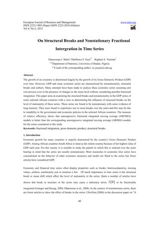
Vol 4, No.5, 2012

where d0 = u + d and u = 1, 2,... depending on the number of the unit differences. The

{φ ,θ } , i = 1,..., p; j = 1,..., q
i j are the parameters in the model and ε t −i are the random process

distributed as εt −i ≈ N ( 0,1) .

5. Source of Data
The data used in this study were the GDP per capita per person in current US Dollar of 27 African countries
from 1960 to 2006. The annual data were sourced from International Monetary Fund (IMF) database. The
GDP data is computed from the purchasing power parity (PPP) of countries per capita, that is the value of
all final goods and services produced within a country in a given year divided by the average or mid-year
population for the same year.

6. Results and Discussion
The time plots of the GDP series for different countries are shown in Figure 1 below. The data used are
given in US dollars in order to allow country to country comparison. Various types of movements were
noticed in the plots of GDP for these countries. A general upward movements were noticed from 1961 for
the next five years, followed by sharp increases from 1966 to 1976 or there about. Thereafter, different
types of movements were exhibited by different countries for the rest of the period under study. Most of the
countries experienced drops in the GDP which may be due to decrease in the values expressed in the
country’s local currency. Nigeria for example experienced significant drops between 1980 and 2003.

43

Vol 4, No.5, 2012

Figure 1: Time Plots of GDP in African Country with figures given in US Dollars

ALGERIA BENIN BURKINA FASO
BOTSWANA

60 65 70 75 80 85 90 95 00 05 60 65 70 75 80 85 90 95 00 05 60 65 70 75 80 85 90 95 00 05
60 65 70 75 80 85 90 95 00 05

BURUNDI CAMEROON CHAD CONGO

60 65 70 75 80 85 90 95 00 05
60 65 70 75 80 85 90 95 00 05
60 65 70 75 80 85 90 95 00 05 60 65 70 75 80 85 90 95 00 05

COT E D'VOIRE EGYPT
GABON
GHANA

60 65 70 75 80 85 90 95 00 05 60 65 70 75 80 85 90 95 00 05
60 65 70 75 80 85 90 95 00 05

60 65 70 75 80 85 90 95 00 05

KENYA
LESOT HO LIBERIA
MALAWI

60 65 70 75 80 85 90 95 00 05
60 65 70 75 80 85 90 95 00 05 60 65 70 75 80 85 90 95 00 05
60 65 70 75 80 85 90 95 00 05

MALAYSIA MAURITANIA NIGER NIGERIA

60 65 70 75 80 85 90 95 00 05 60 65 70 75 80 85 90 95 00 05 60 65 70 75 80 85 90 95 00 05
60 65 70 75 80 85 90 95 00 05

SENEGAL SIERRA LEONE SOUT H AFRICA
SUDAN

60 65 70 75 80 85 90 95 00 05 60 65 70 75 80 85 90 95 00 05
60 65 70 75 80 85 90 95 00 05
60 65 70 75 80 85 90 95 00 05

T OGO UGANDA ZAMBIA

60 65 70 75 80 85 90 95 00 05 60 65 70 75 80 85 90 95 00 05 60 65 70 75 80 85 90 95 00 05

44

Vol 4, No.5, 2012

This significant drop experienced in Nigeria is also traced back to the behavior of Naira-US dollar
exchange rates in the period under investigation. In that case, the nominal GDP in Naira is given
below in Figure 2, and this shows astronomical increase of GDP in the country. Comparison of the two
plots of GDP for Nigeria shows that exchange rate has effect on the country’s wealth.

Figure 2: Time plot of Nigerian (nominal) GDP in millions of Naira

NIGERIA
20,000,000

16,000,000

12,000,000

8,000,000

4,000,000

0
60 62 64 66 68 70 72 74 76 78 80 82 84 86 88 90 92 94 96 98 00 02 04 06

From Table 1, the ADF unit root test shows that all the series are nonstationary at 5% level of
significance. However, all the series attained stationarity after the first difference. The above shows

that the GDP series are integrated of order one, I (1) . This suggests that the series can be modelled as

ARIMA (p, d, q). Shittu and Yaya (2009, 2010) showed that under certain conditions, ARFIMA model
may be better than ARIMA model when nonstationarity is established in a series.
Table 1: Unit root tests on GDP series
Observed Series First Differenced Observed Series First Differenced
Countries ADF Prob. ADF Series Prob. Countries ADF Prob. ADF Series Prob.
Algeria Statistic
-0.9247 (5%)
0.7708 Statistic
-4.4448 (5%)
0.0009 Liberia Statistic
-1.6164 (5%)
0.4661 Statistic
-4.0992 (5%)
0.0024
Benin -0.1828 0.9333 -7.3291 0.0000 Malawi -1.6899 0.4295 -7.4282 0.0000
Botswana 2.1849 0.9999 -4.4063 0.0008 Malaysia 0.9706 0.9956 -4.9800 0.0002
Burkina -0.2051 0.9303 -5.1443 0.0001 Mauritania -0.0865 0.9447 -3.5398 0.0113
Faso
Burundi -1.2956 0.6236 -5.1480 0.0001 Niger -2.5505 0.1108 -4.6275 0.0005
Cameroon -0.9280 0.7704 -5.9970 0.0000 Nigeria -0.5198 0.5146 -4.4185 0.0009
Chad -0.5889 0.8628 -3.5435 0.0111 Senegal -0.9562 0.7609 -5.6289 0.0000
Congo 0.6859 0.9906 -4.4716 0.0008 Sierra -2.1146 0.2401 -6.3065 0.0000
Cote -1.8459 0.3542 -4.6347 0.0005 Leone
South -0.5501 0.8713 -4.6040 0.0005
D'vore
Egypt 2.5622 1.0000 -4.0914 0.0025 Africa
Sudan -0.1286 0.9399 -6.0260 0.0000
Gabon -0.8763 0.7869 -5.3685 0.0001 Togo -1.7109 0.4192 -5.3715 0.0000
Ghana -0.7451 0.8248 -5.3252 0.0001 Uganda -2.4599 0.1319 -4.9790 0.0002
Kenya -0.1854 0.9326 -4.2919 0.0014 Zambia -1.6277 0.4604 -2.9934 0.0431
Lesotho 0.4566 0.9833 -4.8220 0.0003

45

Vol 4, No.5, 2012

With this in mind, we examined whether or not all the series were actually I ( 0) or I ( d ) where d is

the fractional difference parameter for all the series. The result is shown in Table 3.

Table 3: Estimates of Fractional Difference Parameter
Burkina Côte
Country Algeria Benin Botswana Burundi Cameroon Chad Congo
Faso D'Ivoire
dˆ 1.1039 1.0108 1.0801 1.0182 1.1357 1.0785 1.1029 1.0498 1.1158
Country Egypt Gabon Ghana Kenya Lesotho Liberia Malawi Malaysia Mauritania
dˆ 1.0485 1.0546 1.0361 1.1048 1.0097 1.1258 0.9111 0.9684 1.0465
Sierra South
Country Niger Nigeria Senegal Sudan Togo Uganda Zambia
Leone Africa
dˆ 1.0950 1.1265 0.9839 1.0248 1.0505 1.0641 1.0287 0.9996 1.0678

It can be observed that all the series were not exactly of order one, I (1) .

6.1 Investigation of Structural Breaks
The first value corresponds to the estimate of d based on the sample with the first 35 observations, that
is, from 1960 to 1994, then the following one corresponds to the sample [1961 – 1995], the next.
[1962 – 1996] and so on till the last one which corresponds to [1972 – 2006] making 13 blocks of
samples i.e. 1960 – 1994, 1961 – 1995, 1962 – 1996, 1963 – 1997, 1964 – 1998, 1965 – 1999,
1966 – 2000, 1967 – 2001, 1968 – 2002, 1969 – 2003, 1970 – 2004, 1971 – 2005, 1972 – 2006. The

following figure displays for each country the estimates of differencing parameters d0 along with

the 95% confidence band using the model in (1).

Stable estimates of d across the different subsamples are observed in the GDP of Burundi, Cameroon,
Gabon, Kenya, Liberia, Niger, Nigeria, Sierra Leone and Uganda. In Benin, Bostwana, Lesotho and
South Africa, we notice a decrease in the degree of integration about the 10th estimate [2003]. A slight
increase in the estimated value of d about the 10th / 11th estimate [2003, 2004] is observed in Algeria,
Chad, Congo, Sudan and Zambia. In fact, in the above 10 countries, we observe a sharp increase about
the year 2003.

For another group, we observe a slight decrease in the 2nd estimate [1995]. This group include
Burkina Faso, Cote de Ivory, Senegal and Togo. For Ghana and Malawi, break is observed in the 8th
block [2001].

46

Vol 4, No.5, 2012

47

Vol 4, No.5, 2012

6.2 Modelling of the Series
To determine the most appropriate model for GDP series in the selected countries in Africa, the ARIMA (p,
d, q) and ARFIMA (p, d, q) modelling were carried out on the series with a view to measure the relative
efficiency (R.E) of the ARFIMA model over the ARIMA model. The results are shown in Table 4
and 5 below.

Table 4: Estimated Nonstationary ARFIMA Models for the African GDP Series

1 .2 0 86
 0 .1 18 1
 
y t = (1 − B ) Xt

Algeria yt = 0.4684 yt −3 + 0.2607 yt −6 − 0.4382 yt −9 − 0.2650 yt −13 + εt
0.1474
  0.1579
  0.1504
  0.1469
 

Sk. = -0.5328 Ex. Kurt. = 3.0732 ARCH = 1.8621 [0.1535] σ ARFIMA = 24026.4
2
σ ARIMA = 27792
2
σ ARFIMA ARIMA = 0.8645
2

1.1 4 94
 0 .0 99 0 
 
y t = (1 − B ) Xt

Benin yt = − 0.4860 yt −4 − 0.2694 yt −10 + 0.3748 yt −13 − 0.7577 yt −14 + 0.4421 yt −15 + εt
0.1359
  0.1433
  0.1755
  0.2146
  0.2217
 

2
σ ARIMA =
2
1026.95 σ ARFIMA ARIMA = 0.9483
2

1.0 0 00
 0 .0 00 0 
 
y t = (1 − B ) Xt

Botswana yt = 1.6497+ 0.6106 yt −1 − 0.5397 yt −2 + 0.4146 yt −3 − 0.3829 yt −6 − 0.6347 yt −12 + 1.3092 yt −13 − 1.0303 yt −14 + 1.3597 yt −15 + εt
0.0000
  0.1150
  0.1300
  0.1256
  0.1831
  0.2350
  0.2837
  0.3086
  0.2612
 

2
σ ARIMA = 25905.8
2
2

1 .27 8 6
 0 .1 15 3 
 
y t = (1 − B ) Xt

yt = −0.4572 yt −4 − 0.2769 yt −6 − 0.3706 yt −10 − 0.5152 yt −14 + 0.3825 yt −15 + εt
Burkina Faso 0.1408
 0.1445
  0.1504
  0.1742
  0.2347
 


2
σ ARIMA = 693.206
2
2

− 1 .19 0 4
 0 .3 80 3 
 
y t = (1 − B ) Xt

Burundi yt = 131.79− 1.9205 yt −1 − 0.9635 yt −2 + 0.2227 yt −6 − 0.4155 yt −7 + 0.2734 yt −8 − 0.4393 yt −13 + 0.5748 yt −14 − 0.1857 yt −15 + εt
0.2951
  0.2951
  0.3333
  0.1936
  0.2804
  0.1662
  0.1616
  0.2637
  0.1381
 

Sk. = 0.2042 Ex. Kurt. = 1.7494 ARCH = 0.8209 [0.4914] σ ARFIMA = 57436.8
2
σ ARIMA = 59764.3 σ ARFIMA ARIMA = 0.9611
2 2

48

Vol 4, No.5, 2012

0 .84 5 4
 0 .1 08 8 
 
y t = (1 − B ) Xt

yt = 2064.90+ 0.1797 yt −2 + 0.2579 yt −5 + 0.2192 yt −6 − 0.3466 yt −8 − 0.2917 yt −11 + 0.3380 yt −13 − 0.4426 yt −14 + εt
Cameroon 750.5
  0.1286
 0.1387
  0.1332
  0.1431
  0.1407
  0.1974
  0.2012
 


2
σ ARIMA =
2
5141.69 σ ARFIMA ARIMA = 0.0162
2

1 .4 05 6
 0 .2 76 5 
 
y t = (1 − B ) Xt

Chad yt = 903.584+ 0.3230 yt −1 − 0.2158 yt −9 − 0.5773 yt −11 + 0.6543 yt −13 − 0.1492 yt −15 + εt
713.9
  0.2666
  0.1694
  0.1657
  0.1820
  0.1343
 

2
σ ARIMA =
2
745.225 σ ARFIMA ARIMA = 0.9445
2

0 .9 99 9
 0 .0 00 0 
 
y t = (1 − B ) Xt

yt = 2.8E + 07+ 0.3058 yt −1 + 0.2137 yt −4 + 0.3212 yt −5 − 0.3148 yt −6 − 0.3848 yt −12 − 0.5799 yt −13 − 0.3909 yt −14 + 0.7431 yt −15 + εt
0.0000
  0.1324
  0.1354
  0.1316
  0.1448
  0.1677
  0.1635
  0.2004
  0.2120
 
Congo

2
σ ARIMA = 98822.18
2
2

− 0 .8 55 0
 0 .2 42 5 
 
y t = (1 − B ) Xt

Cote D'vore yt = 667.115+ 1.7688 yt −1 − 0.9073 yt −2 + 0.1078 yt −5 + εt
22.55
  0.1900
  0.1732
  0.0315
 

2
2 2

0 .00 0 3
 0 .5 55 0 
 
y t = (1 − B ) Xt

Egypt yt = 9539.39+ 0.5071 yt −1 + 0.6486 yt −3 − 0.2382 yt −4 + εt
702.6
  0.2304
  0.1469
  0.1238
 

Sk. = 0.3858 Ex. Kurt. = 0.0884 ARCH = 0.5362 [0.6604] σ ARFIMA = 369149
2
σ ARIMA = 431325
2
2

0 .50 7 1
 0 .2 47 2 
 
y t = (1 − B ) Xt

Gabon yt = 240208+ 1.1412 yt −1 − 0.2260 yt −4 − 0.2446 yt −6 + 0.2956 yt −9 + 0.7712 yt −10 − 0.4994 yt −12 − 0.2381 yt −14 + εt
1676
  0.0814
  0.1598
  0.2092
  0.2745
  0.2363
  0.2732
  0.1856
 

2
σ ARIMA = 385109 σ ARFIMA ARIMA = 0.0061
2 2

1 .19 4 7
 0 .0 89 5 
 
Ghana y t = (1 − B ) Xt

49

Vol 4, No.5, 2012

yt = − 0.3243 yt −2 − 0.3836 yt −3 − 0.4246 yt −4 − 0.4651 yt −5 − 0.3290 yt −6 − 0.6226 yt −14 + 0.3669 yt −15 + εt
0.1521
  0.1470
  0.1549
  0.1530
  0.1591
  0.1746
  0.1906
 

Sk. =- 0.5379 Ex. Kurt. = 0.2612 ARCH = 0.4112 [0.7460] σ ARFIMA = 870.617
2
2 2

− 0 .10 7 9
 0 .0 96 3 
 
y t = (1 − B ) Xt

Kenya yt = 516.274+ 1.1268 yt −1 − 0.5641 yt −3 − 0.3305 yt −4 + 0.0839 yt −9 − 0.8004 yt −13 + 0.7603 yt −14 + εt
139.6
  0.0886
  0.1502
  0.1242
  0.0541
  0.1340
  0.1263
 

2
σ ARIMA = 686.408
2
2

− 1.1 6 97
 0 .1 23 7 
 
y t = (1 − B ) Xt

Lesotho yt = 302.755+ 1.8804 yt −1 − 1.0093 yt −2 + 0.2157 yt −6 − 0.1757 yt −9 + 0.2718 yt −12 − 0.2060 yt −15 + εt
76.47
  0.1107
  0.1292
  0.0752
  0.0931
  0.0871
  0.0471
 

2
σ ARIMA =
2
1744.13 σ ARFIMA ARIMA = 0.5892
2

− 0.7 0 04
 0 .1 58 0 
 
y t = (1 − B ) Xt

Liberia yt = 293.397+ 1.5866 yt −1 − 0.7066 yt −2 + 0.1679 yt −13 − 0.2869 yt −14 + εt
3.307
  0.1181
  0.0962
  0.1006
  0.1291
 

Sk. = -1.2088 Ex. Kurt. = 5.7365 ARCH = 2.2433 [0.0.0000] σ ARFIMA = 741.198
2
σ ARIMA =
2
1243.01 σ ARFIMA ARIMA = 0.5963
2

− 0 .02 4 9
 0 .2 05 3 
 
y t = (1 − B ) Xt

yt = 177.192+ 0.5780 yt −1 − 0.2957 yt −2 + 0.3326 yt −6 − 0.3023 yt −7 + 0.6015 yt −9 − 0.7598 yt −10 + 1.2405 yt −13 − 0.9110 yt −14 + εt
16.25
  0.1804
  0.1230
  0.1282
  0.1301
  0.1548
  0.1757
  0.2911
  0.2630
 
Malawi

2
2 2

− 0 .0 39 9
 0 .0 15 8 
 
y t = (1 − B ) Xt

Malaysia yt = −16511+ 1.1310 yt −1 − 0.5538 yt −2 + 0.3311 yt −3 − 0.4766 yt −6 + 0.5520 yt −7 − 0.4791 yt −8 + 05175 yt −9 + εt
354.9
  0.1340
  0.1953
  0.1410
  0.1447
  0.2190
  0.2273
  0.1521
 

Sk. = 0.4675 Ex. Kurt. = 1.3541 ARCH = 1.4290 [0.2531] σ ARFIMA = 344.225 σ ARIMA = 70358.4 σ ARFIMA ARIMA = 0.0049
2 2 2

1 .2 18 0
 0 .1 07 8 
 
y t = (1 − B ) Xt
Mauritania
yt = 0.2634 yt −5 − 0.4700 yt −6 − 0.3856 yt −7 − 0.4677 yt −8 − 0.2837 yt −9 − 0.4916 yt −10 + 0.9912 yt −15 + εt
0.1549
  0.1466
  0.1524
  0.1620
  0.1684
  0.1693
  0.3031
 

50

Vol 4, No.5, 2012

2
σ ARIMA = 1673.63
2
2

− 0 .67 9 3
 0 .2 33 5 
 
y t = (1 − B ) Xt

Niger yt = 231.022+ 1.7400 yt −1 − 0.8326 yt −2 − 0.3856 yt −7 − 0.4677 yt −8 − 0.2837 yt −9 − 0.4916 yt −10 + 0.9912 yt −15 + εt
7.295
  0.1681
  0.1628
  0.1524
  0.1620
  0.1684
  0.1693
  0.3031
 

2
2 2

− 0 .23 6 7
 0 .1 52 0 
 
y t = (1 − B ) Xt

Nigeria yt = 367.169+ 1.35327 yt −1 − 0.5931 yt −2 − 0.0570 yt −6 − 0.1975 yt −12 + 0.3115 yt −14 − 0.2621 yt −15 + εt
16.38
  0.1724
  0.1497
  0.0662
  0.08571
  0.1606
  0.1230
 

2
2 2

0 .2 07 4
 0 .2 68 2 
 
y t = (1 − B ) Xt

Senegal yt = 668.380+ 0.8240 yt −1 − 0.3064 yt −2 + 0.2723 yt −3 − 0.2773 yt −4 + 0.2744 yt −13 − 0.3983 yt −14 + 0.2262 yt −15 + εt
120.1
  0.2472
  0.1848
  0.1781
  0.1426
  0.1866
  0.2278
  0.1253
 

2
2 2

− 0 .5 45 4
 0 .1 82 8 
 
y t = (1 − B ) Xt

Sierra Leone yt = 210.744+ 1.1793 yt −1 − 0.3563 yt −2 − 0.2995 yt −8 + 0.5308 yt −9 − 0.3600 yt −10 + 0.2756 yt −14 − 0.2918 yt −15 + εt
3.800
  0.1756
  0.1393
  0.1318
  0.2009
  0.1407
  0.1301
  0.1182
 

2
σ ARIMA = 1119.07
2
2

0 .0 00 7
 0 .0 00 8 
 
y t = (1 − B ) Xt

South Africa yt = −102905+ 1.3083 yt −1 − 0.5221 yt −2 − 0.3280 yt −5 + 0.5787 yt −6 − 0.4823 yt −7 + 0.6697 yt −8 − 0.5150 yt −9 + 0.2907 yt −11 + εt
3255
  0.1337
  0.1536
  0.1895
  0.2752
  0.2856
  0.2789
  0.2290
  0.1307
 

Sk. =-0.3446 Ex. Kurt. = 0.4664 ARCH = 1.8418 [0.1601] σ ARFIMA = 64656
2
σ ARIMA = 87353 σ ARFIMA ARIMA = 0.7402
2 2

− 0 .5 03 2
 0 .1 52 5 
 
y t = (1 − B ) Xt

Sudan yt = 431.490+ 1.3176 yt −1 − 0.4135 yt −3 + 0.1427 yt −8 − 0.2083 yt −11 + 0.1329 yt −15 + εt
75.69
  0.1003
  0.1041
  0.0748
  0.0806
  0.0462
 

2
σ ARIMA =
2
8511.1 σ ARFIMA ARIMA = 0.7716
2

51

Vol 4, No.5, 2012

0 .5 46 3
 0 .2 22 3 
 
y t = (1 − B ) Xt

Togo yt = 23.9437+ 0.6282 yt −1 + 0.4044 yt −12 − 0.3241 yt −13 − 0.3058 yt −14 + 0.4967 yt −15 + εt
161.7
  0.2018
  0.1391
  0.1876
  0.1888
  0.1644
 

Sk. = -0.12717 Ex. Kurt. = 1.6211 ARCH = 2.3798 [0.0868] σ ARFIMA = 986.417 σ ARIMA = 1047.13 σ ARFIMA ARIMA = 0.9420
2 2 2

0 .2 33 2
 0 .1 43 2 
 
y t = (1 − B ) Xt

Uganda yt = 237.479+ 1.0418 yt −1 − 0.2862 yt −2 − 0.3745 yt −4 + 0.3871 yt −5 − 0.3573 yt −6 + 0.2304 yt −7 + εt
16.16
  0.1380
  0.1547
  0.1522
  0.2020
  0.1995
  0.1313
 

2
2 2

0 .4 32 4
 0 .0 67 6 
 
y t = (1 − B ) Xt

Zambia yt = 459.367+ 1.3991 yt −1 − 0.6012 yt −2 − 0.1563 yt −10 + εt
31.00
  0.1554
  0.1623
  0.1037
 

2
σ ARIMA = 4341.06
2
2

The relative efficiency between the ARFIMA (p, d, q) and ARIMA (p, d, q) are given in Table 5.

52

11.on structural breaks and nonstationary fractional intergration in time series

11.on structural breaks and nonstationary fractional intergration in time series

Recommended

Recommended

More Related Content

What's hot

What's hot (16)

Similar to 11.on structural breaks and nonstationary fractional intergration in time series

Similar to 11.on structural breaks and nonstationary fractional intergration in time series (20)

More from Alexander Decker

More from Alexander Decker (20)

Recently uploaded

Recently uploaded (20)

11.on structural breaks and nonstationary fractional intergration in time series