This study examines factors that influence real exchange rates in Asian economies including Japan, Korea, and Hong Kong. The methods show that real exchange rates and terms of trade can be jointly determined. Productivity differential, terms of trade, real oil prices, and reserve differentials are found to impact real exchange rates in these economies in the long run, though the impacts vary between economies. The factors influencing real exchange rate determination also differ depending on the economy's exchange rate regime and degree of openness to trade.

1. The real exchange rate determination: An empirical investigation
Wong Hock Tsen ⁎
School of Business and Economics, Universiti Malaysia Sabah, Locked Bag No. 2073, 88999 Kota Kinabalu, Sabah, Malaysia
a r t i c l e i n f o a b s t r a c t
Article history:
Received 18 February 2010
Received in revised form 7 February 2011
Accepted 7 February 2011
Available online 13 February 2011
This study examines the real exchange rate determination in Asian economies. The methods
show that the real exchange rate and terms of trade can be jointly determined. Productivity
differential, terms of trade, the real oil price, and reserve differential are found to be important
in the real exchange rate determination in the long run. However, the significant impacts of
those variables on the real exchange rate determination are different across economies.
Moreover, the results of the generalised forecast error variance decompositions show that the
important contributors of the real exchange rate are different across economies.
© 2011 Elsevier Inc. All rights reserved.
JEL classification:
F31
F37
F10
Keywords:
Real exchange rate
Terms of trade
Reserve differential
Real oil price
Cointegration
1. Introduction
The real exchange rate plays an important role in the international trade and investment determination. Appreciation of the real
exchange rate could retard exports and inflows of foreign direct investment and thus economics growth can be affected. Moreover, the
real exchange rate is argued to influence balance of payment of a country. Therefore it is important to determine factors that influence the
real exchange rate (Miyakoshi, 2003: 173). A suitable or targeted level of the real exchange rate can be achieved through influencing the
real exchange rate determinants. There are a number of views on the real exchange rate determination (Copeland, 2008; Williamson,
2009). Miyakoshi (2003) shows that productivity differential is important in the real exchange rate determination for some countries
whilst the real interest rate differential is more important in the real exchange rate determination for other countries. Wang and Dunne
(2003) show that fundamentals or real variables explain some but not all the variations of the real exchange rates and different
disturbances have different degrees of importance for different real exchange rates. There is no universal panacea for changes in the real
exchange rate. This issue remains open and little consensus exists on the factors that influence the real exchange rate.
There are some important factors that influence the real exchange rate but not considered in some of previous studies (Miyakoshi,
2003; Wang & Dunne, 2003). Amano and Van Norden (1995), Karfakis and Phipps (1999), Aruman and Dungey (2003), and Bleaney and
Francisco (2010), amongst others, present the evidence of the strong relationship between the real exchange rate and terms of trade. De
Gregorio and Wolf (1994) demonstrate that, amongst others, improved terms of trade will lead to an appreciation of the real exchange
rate. The impact of terms of trade on the real exchange rate is found to be stronger than the impact of the expected real interest
differential.1
In contrast, Gruen and Wilkinson (1994) report that the real interest rate differential is qualitatively more important than
International Review of Economics and Finance 20 (2011) 800–811
⁎ Tel.: +60 88 320000x1616.
E-mail address: htwong@ums.edu.my.
1
The expected real interest rate differential captures financial market development particularly capital flows and terms of trade captures good markets
development (Bagchi, Chortareas, & Miller, 2004: 77).
1059-0560/$ – see front matter © 2011 Elsevier Inc. All rights reserved.
doi:10.1016/j.iref.2011.02.002
Contents lists available at ScienceDirect
International Review of Economics and Finance
journal homepage: www.elsevier.com/locate/iref

2. terms of trade in explaining the real exchange rate.2
Reserve differential could influence the real exchange rate. A country with a high
international net-asset position tends to have a strong currency whereas a country with a low international net-asset position tends to
have a weak currency. One way to increase international net-asset position is to increase exports through depreciation of the real
exchange rate (Wang, Hui, & Soofi, 2007; Aizenman & Riera-Crichton, 2008).
This study examines the real exchange rate determination in Asian economies, namely Japan, Korea, and Hong Kong. These
economies adopt different exchange rate regimes and trade openness is not the same. Japan and Korea adopt an independently
floating exchange rate regime most of the time, which exchange rate is market-determined and official foreign exchange market
intervention is aimed to moderate the rate of change and not to set a level for it. Hong Kong adopts a currency board arrangement
most of the time, which an explicit legislative commitment to exchange domestic currency for a specified foreign currency at a
fixed exchange rate is carried out (Fischer, 2008). Japan is relatively a closed economy. Korea and Hong Kong are relatively open
economies. Trade openness, namely exports plus imports of goods and services to Gross Domestic Product (GDP) of Japan was
25.8% for the period 1960–2008. For Korea and Hong Kong, the trade openness ratios were 70.5% and 295.8% for the same period,
respectively (Table 1). Hence this study provides some evidence of the real exchange rate determination in different exchange rate
regimes and different degrees of trade openness. More precisely, this study estimates the real exchange rate model of Chen and
Chen (2007) augmented by terms of trade and reserve differential.3
These two variables are not examined in many previous
studies. Moreover, this study examines the period including the Asian financial crisis period, 1997–1998 whereas many previous
studies cover up to the period before the crisis (Miyakoshi, 2003; Wang & Dunne, 2003). The residual based tests for cointegration
with the Generalised Least Squares (GLS) detrended data of the Elliot et al. (1996) (ERS) is used in addition to the uses of the
Johansen (1988) cointegration method and the Saikkonen and Lütkepohl (2000) (SL) cointegration method to examine the
cointegration of the variables in this study.
The rest of this study is structured as follows. Section 2 gives a literature review of the real exchange rate determination.
Section 3 explains the data and methodology used in this study and Section 4 presents empirical results and discussions. The last
section includes some concluding remarks.
2. A literature review
The Balassa (1964) and Samuelson (1964) (BS) hypothesis argue that an increase in productivity differential of traded goods to
non-traded goods will lead to appreciation of the real exchange rate. Miyakoshi (2003) examines the real exchange rate
determination between Japan and East-Asian countries, namely Korea, Malaysia, Indonesia, and the Philippines. Productivity
differential is found to be more important in the real exchange rates of Indonesia and the Philippines against Japanese yen,
respectively whilst the real interest rate differential is found to be more important in the real exchange rates of Korea, Malaysia,
and Indonesia against Japanese yen, respectively. Generally, productivity differential and the real interest rate differential shall be
considered when estimating the real exchange rates. In contrast, Wang and Dunne (2003) investigate the dynamic of the real
exchange rates in East Asia, namely Japan, Korea, Malaysia, Singapore, Indonesia, the Philippines, and Thailand. The results of
generalised variance decompositions demonstrate that fundamentals such as productivity differential explain some but not all the
variations of the real exchange rates and different factors have different degrees of importance for each real exchange rate.
Moreover, Lee, Nziramasanga, and Ahn (2002) find the real variables, namely terms of trade and industry productivity to have
long-run impacts on the real exchange rate whereas the nominal variables, namely relative money supply and current account to
have short-run impacts on the real exchange rate between New Zealand and Australia. Chinn (2000), Choudhri and Khan (2005),
Egert, Lommatzsch, and Lahreche-Revil (2006), and Guo (2010), amongst others, find the importance of the BS hypothesis in the
real exchange rate determination.
Table 1
Trade openness.
Year Japan Korea Hong Kong
1960–1969 19.5 26.5 163.4
1970–1979 22.9 56.0 187.1
1980–1989 23.4 69.1 209.5
1990–1999 18.4 61.5 265.1
2000–2005 22.8 76.8 322.4
2006 30.9 85.1 399.5
2007 34.0 82.3 405.3
2008 34.2 107.0 414.1
Note: Trade openness is measured by exports plus imports of goods and services divided by GDP and multiplied by 100.
2
Chen (2006) examines the nexus of interest rate and exchange rate and the effectiveness of interest rate defence in six developing countries (Indonesia,
Korea, the Philippines, Thailand, Mexico, and Turkey). The results of the Markov-switching specification of the nominal exchange rate with the transition
probabilities assumed time varying show that an increase in interest rate will lead to a higher probability of switching to a crisis regime. Thus high interest rate
policy may be unable to defend exchange rate. Moreover, a high interest rate would lead to a high exchange rate volatility (Chen, 2007).
3
Cavallo and Ghironi (2002) develop a two-country monetary model with incomplete asset markets, stationary net-foreign assets, and endogenous monetary
policy. The model de-emphasises the role of exogenous money supply and emphasises the relationship between the exchange rate and the net-foreign assets and
the endogeneity of interest rate setting in exchange rate determination.
801W.H. Tsen / International Review of Economics and Finance 20 (2011) 800–811

3. Chen and Chen (2007) study the impacts of the real oil prices on the real exchange rates in the G7 countries, namely Canada,
France, Germany, Italy, Japan, the United Kingdom, and the United States (US). The results of the Johansen (1988) cointegration
method exhibit that there is a link between the real oil price and the real exchange rate. Moreover, the panel predictive regression
suggests the real oil price has a significant forecasting power. Furthermore, the results show the real interest rate differential and
productivity differential to have significant impacts on the real exchange rate. The real oil price is important in the exchange rate
determination. Korhonen and Juurikkala (2009) examine the real exchange rate determination in a sample of oil-dependent
countries, namely Organisation of the Petroleum Exporting Countries (OPEC). The real exchange rate is specified as a function of
real GDP per capita and the real oil price. The results of the pooled mean group and mean group estimators reveal that an increase
in the real oil price will lead to appreciation of the real exchange rate. The elasticity of the real oil price is typically between 0.4 and
0.5 but would be larger depending upon the specification. On the other hand, real GDP per capita does not appear to have a
significant effect on the real exchange rate. Conversely, Lizardo and Mollick (2010) find that the impact of the real oil price on the
real exchange rate differ across economies. An increase in the real oil price will lead to significant depreciation of the US dollar
against the net-oil exporter currencies, such as Canada, Mexico, and Russia. In contrast, an increase in the real oil price will lead to
significant depreciation of the net-oil importer currencies against the US dollar, such as Japan.
Amano and Van Norden (1995) reveal the real exchange rate and terms of trade are cointegrated in Canada and the US.
Moreover, much of the variation in the real exchange rate is attributable to the movements in terms of trade and the influence of
interest rate differential is secondary. Bagchi et al. (2004) investigate the impacts of the expected real interest rate differential and
terms of trade on the real exchange rate in nine small and developed economies, namely Australia, Australia, Canada, Finland, Italy,
New Zealand, Norway, Portugal, and Spain using the Johansen (1988) cointegration method. The results indicate that the expected
real interest rate differential and terms of trade affect the real exchange rate in the long run but the impact of terms of trade is
generally more consistent. In five economies (Australia, Canada, Finland, Italy, and Portugal), the expected real interest rate
differential possesses the predicted negative relationship with the real exchange rate. In some economies, terms of trade (export
prices divided by import prices) improvement causes appreciation whereas depreciation in other economies. The negative
relationship between terms of trade and the real exchange rate can be explained by incomplete pass-through and or pricing to
market behaviour or local currency pricing behaviour. Bleaney and Francisco (2010) find that, amongst others, the real effective
exchange rate volatility is strongly associated with terms of trade volatility. Karfakis and Phipps (1999), Aruman and Dungey
(2003), and Bergvall (2004), amongst others, report terms of trade to have a significant impact on the real exchange rate.
Aizenman and Riera-Crichton (2008) explore the impacts of international reserve, terms of trade, and capital flows on the real
exchange rate. The results demonstrate that international reserve cushions the impact of terms of trade shock on the real exchange
rate. This effect is important for developing countries especially in Asian and countries exporting natural resources. However, this
buffer effect is not very important for industrial countries. Wang et al. (2007) estimate the real effective exchange rate (REER) of
China as a function of terms of trade, relative prices of the trade goods to non-trade goods, foreign exchange reserve, and the
change of money supply. The results of the Johansen (1988) cointegration method show that, amongst others, an increase in
foreign exchange reserve will lead to an increase in REER. Nonetheless, the impact of international reserve on the real exchange
rate could be differed across economies. Egert et al. (2006) examine the role of productivity, relative prices, and the net-foreign
assets on the real exchange rate determination in a set of transition economies of Central and Eastern Europe and a group of small
Organisation for Economic Cooperation and Development (OECD) countries. For the Baltic countries, an increase in debt will lead
to appreciation of the real exchange rates. For the Central and Eastern European Economies (CEE), an increase in the net-foreign
assets will tend to an appreciation of the real exchange rates in the long run.
3. Data and methodology
The real exchange rate (RERt) is expressed by RERt = ERt ×
CPId;t
CPIus;t
, where ERt is the domestic currency against the US dollar
exchange rate, CPId,t is the domestic Consumer Price Index (CPI, 2000=100), and CPIus,t is the US CPI (2000=100). An increase in
the real exchange rate means depreciation of the real exchange rate in the domestic currency.4
Terms of trade (TOTt) is expressed
by TOTt =
Px;t
Pm;t
, where Px,t is the export price index (2000=100) and Pm,t is the import price index (2000=100). Productivity
differential (PDt) is expressed by PDt =
Yd;t
Nd;t
−
Yus;t
Nus;t
, where Yt is the GDP volume (2000=100), Nt is the manufacturing employment
index (2000=100), and subscripts d and us denote domestic and the US, respectively. The real oil price (Ot) is expressed by the
world oil price index (3 Spot Price Index, 2000=100) divided by the domestic CPI. Reserve differential (RDt) is expressed by
RDt =
Rd;t
Yd;t
−
Rus;t
Yus;t
, where Rt is the real total reserve plus gold (millions of the US dollar) and Yt is real GDP (millions of the US dollar).
The real interest rate differential (DRt) is expressed by (rd,t −rus,t), where rd,t is the real domestic money market rate and rus,t is the
real US federal fund rate. There are two measures of the real interest rate differential used in this study. First, the real interest rate
is expressed by subtracting inflation from the nominal interest rate (Chen & Chen, 2007). Inflation is measured by the change of
CPI (DR1,t). Second, the real interest rate is expressed by subtracting the expected inflation from the nominal interest rate, which
4
The US is an important trading partner of Japan, Korea, and Hong Kong. In 2000, trade of Japan with the US was 25.2% of total trade of Japan. In 2005 and
2008, trades of Japan with the US were 18.2% and 14.1% of total trade of Japan, respectively. For Korea, trades with the US were 20.2%, 13.2%, and 9.9% of total
trade of Korea in 2000, 2005, and 2008, respectively. For Hong Kong, trades with the US were 14.9%, 10.5%, and 8.8% of total trade of Hong Kong in 2000, 2005,
and 2008, respectively (Direction of Trade Statistics, IMF). Patnaik et al. (2011) find that Asia was tightly pegged to the US dollar in the years before the Asian
financial crisis and in some years after the crisis. However, since 2006 Asia has moved away from tight pegging to the US dollar. Nonetheless, the US dollar is still
an anchor currency in a pegged or managed regime.
802 W.H. Tsen / International Review of Economics and Finance 20 (2011) 800–811

4. (a)
-2
0
2
4
6
8
10
65 70 75 80 85 90 95 00 05
RER TOT PD
O RD
-2
0
2
4
6
8
10
80 85 90 95 00 05
RER TOT PD
O RD
Japan Korea
Japan Korea
Hong Kong
Hong Kong
-2
0
2
4
6
8
10
92 94 96 98 00 02 04 06 08
RER TOT PD
O RD
(b)
-12
-8
-4
0
4
8
12
16
20
65 70 75 80 85 90 95 00 05
DR1 DR2
-12
-8
-4
0
4
8
12
16
20
80 85 90 95 00 05
DR1 DR2
-12
-8
-4
0
4
8
12
16
20
92 94 96 98 00 02 04 06 08
DR1 DR2
Fig. 1. (a) The plots of the natural logarithms of the real exchange rate, terms of trade, productivity differential, reserve differential, and the real oil price. (b) The
plots of the real interest rate differentials.
803W.H. Tsen / International Review of Economics and Finance 20 (2011) 800–811

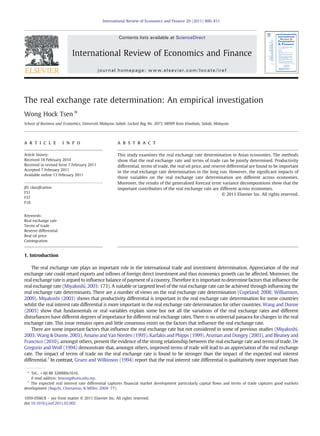
5. the expected inflation is expressed by two-year centred moving average of inflation, incorporating both the backward-looking and
forward-looking elements (Bagchi et al., 2004) (DR2,t). The data were obtained from International Financial Statistics, the
International Monetary Fund (IFS, IMF). The sample periods for Japan, Korea, and Hong Kong are 1960:Q2-2009:Q4, 1976:Q4-
2009:Q4, and 1990:Q4-2009:Q4, respectively.5
The choice of sample period is subject to the availability of all the relevant data. All
data were seasonal adjusted using the Census X12 seasonal adjustment procedure, except that the manufacturing employment
indexes of the US and Japan are originally seasonal adjusted.6
All data were transformed into the natural logarithms before
estimation, except interest rates (the federal fund rate and the money market rate).
Fig. 1(a) displays the plots of the natural logarithms of the real exchange rate, terms of trade, productivity differential, the real
oil price, and reserve differential in Japan, Korea, and Hong Kong whilst Fig. 1(b) displays the plots of the real interest rate
differentials. There was a small jump in the reserve differential in 2007, which could be the result of the weak global economy.
Generally, the real exchange rate, terms of trade, productivity differential, the real oil price, and reserve differential tended to
move in the same direction and tended to be cointegrated. Also, the real interest rate differentials moved closely to each other.
This study estimates the real exchange rate model of Chen and Chen (2007) augmented by terms of trade and reserve
differential. More explicitly, the model to be estimated is specified as follows7 8
:
logRERt = β10 + β11logTOTt + β12logPDt + β13logRDt + u1;t ð1aÞ
logTOTt = β20 + β21logOt + u2;t ð1bÞ
where log is the natural logarithm, RERt is the real exchange rate (the domestic currency against the US dollar), TOTt is terms of
trade, PDt is productivity differential, RDt is reserve differential, Ot is the real oil price, and ui,t (i=1, 2) is a disturbance term. A
dummy variable, that is, one for the period 1997:Q2-1998:Q4 and the rest are zero is also included as a deterministic variable in
the estimation to capture the influence of the Asian financial crisis, 1997–1998. Moreover, the real interest rate differential (DRt) is
included as a deterministic variable in the estimation as it tends to be a stationary variable. The model with the first measure of the
real interest rate differential (DR1,t) is named as model 1 whilst the model with the second measure of the real interest rate
differential (DR2,t) is named as model 2.
Backus and Crucini (2000) use a dynamic general equilibrium model and find that oil price accounted for much of the variation
in terms of trade over the last twenty-five years and its quantitative role varied significantly over time. Moreover, terms of trade of
industrialised countries were driven mainly by changes in oil price for the period 1972–1987. Furthermore, the increased volatility
in terms of trade since the end of the Bretton Woods system seemed largely due to the increased volatility in oil price rather than
the increased volatility of the nominal or real exchange rate. Hence oil price is important in the terms of trade determination. A
change in oil price could affect export price and import price in a different proportion and thus terms of trade will change. The
correlation between terms of trade and oil price is argued to be strong. The correlations between terms of trade and the real oil
price for Japan, Korea, and Hong Kong were −0.9530 (1960:Q1-2009:Q4), −0.2061 (1976:Q1-2009:Q4), and −0.7430 (1990:Q1-
2009:Q4), respectively. The two variables are correlated and putting them in the same side of the equation in the estimation could
lead to the multicollinearity problem. Moreover, the two variables are cointegrated (Table 3).
Generally, an increase in terms of trade, that is, export price is higher than import price, ceteris paribus, more imports can be
exchanged with one unit of export and this implies appreciation of the real exchange rate. Thus the coefficient of terms of trade is
expected to be negative (Bagchi et al., 2004; Bergvall, 2004). The BS hypothesis implies that an increase in productivity differential
will lead to appreciation of the real exchange rate and therefore the coefficient of productivity differential is expected to be
negative (Choudhri & Khan, 2005; Guo, 2010). An increase in international reserve, which could be a result of trade balance
surplus, will lead to appreciation of the real exchange rate. However, an increase in debt is reported to lead to appreciation of the
real exchange rate. Therefore the coefficient of reserve differential could be negative or positive (Egert et al., 2006; Aizenman &
Riera-Crichton, 2008). Generally, an increase in oil price would result in more favourable terms of trade for the net-oil exporting
country but less favourable terms of trade for the net-oil importing country. Japan, Korea, and Hong Kong are generally the net-oil
importing economies. Thus the coefficient of the real oil price is expected to be negative (Bergvall, 2004: 327; Chen & Chen, 2007;
Lizardo & Mollick, 2010).
The Zivot and Andrews (1992) (ZA) unit root test statistics are used to examine the stationary of the data. The ZA unit root test
statistics allowing for one structural break in the variable, which can appear in intercept, trend or both. The breakpoint is selected
where the t-statistic on the coefficient of the autoregressive variable to test where the null hypothesis of a unit root is the most
negative. The ZA unit root test statistics test a unit root against the alternative of a trend stationary process with a structural break.
5
The numbers of observations for Japan, Korea, and Hong Kong are 200, 133, and 77, respectively.
6
The Census X12 seasonal adjustment procedure is a procedure used by the United States Census Bureau to adjust seasonality in data. The use of seasonally
adjusted data shall remove the seasonal pattern in data (Bergvall, 2004: 326).
7
Bagchi, Chortareas, and Miller (2004) estimate the real exchange rate as a function of terms of trade and the expected real interest rate differential. Bergvall
(2004) estimates the real effective exchange rate as a function of terms of trade and oil price. Chen and Chen (2007) estimate the real exchange rate as a function
of the real interest rate differential, productivity differential, and the real oil price.
8
A theoretical explanation of the real exchange rate and terms of trade relationship is given by Devereux and Connolly (1996). There are at least two channels
that terms of trade can influence the real exchange rate. A change in consumer preferences toward domestic output will improve terms of trade and will lead to
appreciation of the real exchange rate in domestic economy. A shift in foreign demand towards its higher value of exports or a commodity price change that
favours the production of domestic economy will improve terms of trade of domestic economy. This will lead to appreciation of the real exchange rate (Sager,
2006: 47).
804 W.H. Tsen / International Review of Economics and Finance 20 (2011) 800–811

6. The ZA unit root test is an augmented Dickey and Fuller (1979) (DF) type endogenous break unit root test. This study uses the
Engle and Granger (1987) (EG) residual based test for cointegration with the GLS detrended data in addition to the Johansen
(1988) cointegration method and the SL cointegration method.9
First the data are detrended using the GLS of ERS and then the EG
residual based test for cointegration is carried out. In the first stage, the Ordinary Least Squares (OLS) estimator is used to estimate
the following model:
y
d
t = β31x
d
t + u3;t ð2Þ
where yt
d
and xt
d
are two detrended variables using the GLS of ERS, respectively. The long-run relationship between the two
variables can be examined using the DF unit root test on the disturbance term, u3,t in Eq. (2) as follows:
u3;t = ρu3;t−1 + ∑
q
i=1
β4iu3;t−i + u4;t ð3Þ
where Δ is the first difference operator and u4,t is a disturbance term. The null hypothesis of no cointegration (H0: ρ=0) is tested
against the alternative hypothesis of cointegration (Ha: ρb0) through the t-test for ρ using specifically derived non-standard
critical values. The Phillips and Perron (1988) (PP) unit root test is also used to test the disturbance term, u3,t in Eq. (2). When the
t-test of the PP shows that the disturbance term, u3,t in Eq. (2) is stationary, this implies that the hypothesis of cointegration is not
rejected. Perron and Rodriguez (2000) show that there is a significant increase in power of residual tests when the GLS detrending
is applied to the variables in the cointegrating regression before the residual (Pesavento, 2007). Pesavento (2007) shows that the
power of the residual based test for cointegration with the GLS detrended data can be higher than the power of system tests for
some values of the nuisance parameter. The critical values for cointegration with the GLS detrended data can be referred in Perron
and Rodriguez (2000).
The generalised forecast error variance decomposition is used to examine the relationship of variables (Koop, Pesaran, & Potter,
1996; Pesaran & Shin, 1998). The generalised forecast error variance decomposition determines the proportion of forecast error
variance in one variable caused by the innovations in other variables. Thus the relative importance of a set of variables that affect a
Table 2
The results of the Zivot and Andrews (1992) (ZA) unit root test statistics.
Crash Break Crash Break Crash Break
Japan Korea Hong Kong
log RERt −4.1879
(1995:Q3)
−4.2358
(1985:Q3)
−3.6006
(1997:Q2)
−3.9409
(1997:Q4)
−3.8434
(1998:Q4)
−2.9816
(2007:Q4)
Δ log RERt −6.5653 ⁎⁎⁎
(1995:Q3)
−6.8790 ⁎⁎⁎
(1995:Q3)
−6.0761 ⁎⁎⁎
(1996:Q2)
−6.1749 ⁎⁎⁎
(2002:Q2)
−4.4430
(1998:Q2)
−5.5377 ⁎⁎
(1998:Q4)
log TOTt −4.0183
(1985:Q3)
−4.1927
(1985:Q3)
−2.1805
(1985:Q4)
−4.1654
(1991:Q1)
−3.7880
(2003:Q4)
−3.4371
(2003:Q4)
Δ log TOTt −8.3293 ⁎⁎⁎
(1983:Q1)
−8.3069 ⁎⁎⁎
(1983:Q1)
−6.9608 ⁎⁎⁎
(1981:Q2)
−7.9092 ⁎⁎⁎
(1980:Q4)
−6.5378 ⁎⁎⁎
(2006:Q2)
−7.1926 ⁎⁎⁎
(1995:Q3)
log PDt −3.4048
(1968:Q4)
−5.8363 ⁎⁎⁎
(1978:Q3)
−2.6104
(1983:Q1)
−2.9973
(1991:Q1)
−4.2516
(2007:Q4)
−3.7862
(1996:Q2)
Δ log PDt −6.9981 ⁎⁎⁎
(1996:Q1)
−7.2841⁎⁎⁎
(1970:Q2)
−11.9830 ⁎⁎⁎
(2006:Q3)
−13.1158 ⁎⁎⁎
(2006:Q3)
−9.5558 ⁎⁎⁎
(2008:Q1)
−15.1073 ⁎⁎⁎
(2007:Q4)
log RDt −2.7688
(2003:Q3)
−3.9593
(1989:Q2)
−3.4476
(2006:Q3)
−3.1546
(1990:Q4)
−11.2204 ⁎⁎⁎
(2007:Q1)
−10.9170 ⁎⁎⁎
(2007:Q1)
Δ log RDt −8.2092 ⁎⁎⁎
(1973:Q1)
−8.3319 ⁎⁎⁎
(1973:Q1)
−6.8665 ⁎⁎⁎
(2006:Q3)
−9.4373 ⁎⁎⁎
(2006:Q4)
−8.9244 ⁎⁎⁎
(2008:Q1)
−12.1393 ⁎⁎⁎
(2007:Q1)
log Ot −3.5830
(1986:Q1)
−3.4604
(1986:Q1)
−3.2499
(2003:Q3)
−4.4501
(1998:Q1)
−4.3286
(2003:Q3)
−5.3670 ⁎⁎
(1999:Q2)
Δ log Ot −9.2829 ⁎⁎⁎
(1981:Q1)
−9.3350 ⁎⁎⁎
(1981:Q1)
−8.1602 ⁎⁎⁎
(1981:Q1)
−8.1438 ⁎⁎⁎
(1981:Q1)
−6.5145 ⁎⁎⁎
(1991:Q1)
−6.5755 ⁎⁎⁎
(1999:Q1)
DR1,t −4.7594
(1997:Q2)
−5.2069 ⁎⁎
(1984:Q4)
−4.6471
(1998:Q3)
−4.5206
(1998:Q3)
−6.2728 ⁎⁎⁎
(1998:Q2)
−7.3983 ⁎⁎⁎
(2007:Q4)
Δ DR1,t −8.4990 ⁎⁎⁎
(1992:Q2)
−8.5491 ⁎⁎⁎
(1975:Q3)
−8.2590 ⁎⁎⁎
(1998:Q3)
−8.3963 ⁎⁎⁎
(1998:Q3)
−8.4960 ⁎⁎⁎
(2008:Q1)
−9.0994 ⁎⁎⁎
(2007:Q3)
DR2,t −4.9741 ⁎⁎
(1977:Q2)
−5.0435
(1977:Q2)
−5.2813 ⁎⁎
(1998:Q2)
−5.1848 ⁎⁎
(1990:Q2)
−6.2173 ⁎⁎⁎
(2006:Q1)
−6.9621 ⁎⁎⁎
(1998:Q2)
Δ DR2,t −8.5510 ⁎⁎⁎
(1991:Q3)
−8.5703 ⁎⁎⁎
(1992:Q2)
−8.8838 ⁎⁎⁎
(1998:Q2)
−8.9891 ⁎⁎⁎
(1998:Q2)
−8.0736⁎⁎⁎
(2002:Q1)
−8.2689⁎⁎⁎
(2006:Q1)
Notes: Crash denotes the ZA unit root test statistic for testing an abrupt change in level but no change in the trend rate. Break denotes the ZA unit root test statistic
for testing changes in level and trend. Values in parentheses are the breaks. The critical values can be obtained from Zivot and Andrews (1992).
⁎⁎ Denotes significance at the 5% level.
⁎⁎⁎ Denotes significance at the 1% level.
9
Hjalmarsson and Osterholm (2007) examine the properties of the maximum eigenvalue and trace tests of the Johansen (1988) cointegration method for
near-integrated variables. The results show that there is a high probability of falsely concluding that there is cointegration for unrelated series. The residual based
tests are argued to be a more robust testing of cointegration for near-integrated variables.
805W.H. Tsen / International Review of Economics and Finance 20 (2011) 800–811

7. variance of another variable is determined. A key feature of the generalised forecast error variance decomposition is that it is
invariant to the ordering of the variables in the vector autoregressive (VAR). Hence it provides robust results than the
orthogonalised method of Sims (1980).
4. Empirical results and discussions
The results of the ZA unit root test statistics are presented in Table 2. The lag lengths used to estimate the ZA unit root test
statistics are based on the t-statistic, that is, the last lag included in the estimation is statistically significant at the 10% level. The
fraction of entries on each end of data to be excluded when examining the breaks is the 10% level. The results of the ZA unit root
test statistic show that all the variables are non-stationary in their levels but become stationary after taking the first differences,
except log PDt (break), DR1,t (break), and DR2,t (crash) of Japan, DR2,t (crash and break) of Korea, log RERt (crash), log RDt (crash and
break), and log Ot (break), DR1,t (crash and break), and DR2,t (crash and break) of Hong Kong. For those variables, it is either no
strong evidence of a unit root or a stationary variable.10
The results of the EG residual based test for cointegration with the GLS detrended data are reported in Table 3. The lag lengths
used to estimate the DF unit root test statistics are based on the Akaike Information Criterion (AIC). The lag lengths used to
compute the PP unit root test statistics are based on the Newey–West automatic bandwidth selection with the maximum lag
length is set to eight. On the whole, the results show that the real exchange rate, terms of trade, productivity differential, and
Table 3
The Engle and Granger (1987) (EG) residual based test for cointegration with the GLS detrended data.
Model 1a Model 1b
DF PP DF PP
Detrended data with constant
Japan −8.2795 ⁎⁎⁎(1) −13.1699 ⁎⁎⁎(0) −12.8220 ⁎⁎⁎(0) −12.8160 ⁎⁎⁎(1)
Korea −8.6808 ⁎⁎⁎(0) −8.4303 ⁎⁎⁎(0) −6.5195 ⁎⁎⁎(3) −8.3989 ⁎⁎⁎(8)
Hong Kong −1.8234 ⁎(4) −9.6085 ⁎⁎⁎(4) −1.7264 ⁎(4) −9.1435 ⁎⁎⁎(5)
Detrended data with constant and trend
Japan −4.5825 ⁎⁎⁎(7) −6.6278 ⁎⁎⁎(7) −6.3585 ⁎⁎⁎(7) −11.8618 ⁎⁎⁎(8)
Korea −7.6394 ⁎⁎⁎(0) −7.6290 ⁎⁎⁎(4) −6.4836 ⁎⁎⁎(4) −9.2481 ⁎⁎⁎(5)
Hong Kong −6.7953 ⁎⁎⁎(0) −6.8330 ⁎⁎⁎(3) −6.7856 ⁎⁎⁎(0) −6.8663 ⁎⁎⁎(3)
Notes: Values in parentheses are the lag length used in the estimation of the DF or PP unit root test statistic. The critical values can be obtained from Perron and
Rodriguez (2000).
⁎ Denotes significance at the 10% level.
⁎⁎⁎ Denotes significance at the 1% level.
Table 4
The results of the likelihood ratio test statistics (Johansen, 1988).
Model λMax test statistic λTrace test statistic
H0 r=0 rb=1 rb=2 rb=3 rb=4 r=0 rb=1 rb=2 rb=3 rb=4
Ha r=1 r=2 r=3 r=4 r=5 r≥1 r≥2 r≥3 r≥4 r=5
Japan
1 46.32 ⁎⁎ 24.81 13.85 1.12 0.001 86.10 ⁎⁎ 39.78 14.98 1.21 0.001
2 50.58 ⁎⁎ 22.23 13.79 1.75 0.11 88.46 ⁎⁎ 37.88 15.65 1.87 0.11
Korea
1 28.49 18.33 14.49 6.84 0.41 68.57 ⁎ 40.08 21.74 7.25 0.41
2 28.49 21.52 15.74 4.70 0.33 70.79 ⁎⁎ 42.29 20.77 5.02 0.33
Hong Kong
1 39.30 ⁎⁎ 25.33 ⁎ 13.51 8.87 0.68 87.70 ⁎⁎ 48.40 ⁎ 23.07 9.55 0.68
2 37.60 ⁎⁎ 22.16 9.24 7.50 0.11 76.62 ⁎⁎ 39.02 16.86 7.62 0.12
c.v. 1 33.64 27.42 21.12 14.88 8.07 70.49 48.88 31.54 17.86 8.07
c.v. 2 31.02 24.99 19.02 12.98 6.50 66.23 45.70 28.78 15.75 6.50
Notes: The VAR=4, VAR=4, and VAR=1 are used in the estimation for Japan, Korea, and Hong Kong, respectively. c.v. 1 (c.v. 2) denotes the 5% (10%) critical
value. The critical values can be obtained from Pesaran, Shin, and Smith (2000).
⁎ Denotes significance at the 10% level.
⁎⁎ Denotes significance at the 5% level.
10
The Elliot, Rothenberg, and Stock (1996) (ERS) and Phillips and Perron (1988) (PP) unit root test statistics are also used to examine the stationary of the data.
The lag lengths used to estimate the ERS unit root test statistics are based on the Akaike Information Criterion (AIC). The lag lengths used to compute the PP unit
root test statistics are based on the Newey–West automatic bandwidth selection with the maximum lag length is set to eight. The results of the ERS and PP unit
root test statistics, which are not reported, display that generally all the variables are non-stationary in their levels but become stationary after taking the first
differences, except the real interest rate differential. Moreover, the results of the Lee and Strazicich (2004) unit root test statistics for a structural break, which are
not reported, show about the same conclusion as the ZA unit root test statistics.
806 W.H. Tsen / International Review of Economics and Finance 20 (2011) 800–811

8. reserve differential are cointegrated (Model 1a). Moreover, terms of trade and the real oil price are cointegrated (Model 1b). The
results of the Johansen (1988) cointegration method are reported in Table 4. The results of the λMax and λTrace test statistics are
computed with unrestricted intercepts and no trends in the VAR. The choices of the lag lengths used in the estimation of the test
statistics are based on the AIC. However for Hong Kong, the choices of the lag lengths used in the estimation of the test statistics are
Table 5
The results of the likelihood ratio test statistic (Saikkonen & Lütkepohl, 2000).
Model λTrace test statistic
H0 r=0 rb=1 rb=2 rb=3 rb=4
Ha r=1 r=2 r=3 r=4 r=5
Japan
1 63.44 ⁎⁎ 37.27 ⁎ 16.96 4.08 0.74
Korea
2 66.48 ⁎⁎ 32.63 17.94 6.13 0.01
Hong Kong
1 61.91 ⁎⁎ 27.40 9.52 3.23 0.15
c.v. 1 59.95 40.07 24.16 12.26 4.13
c.v. 2 56.28 37.04 21.76 10.47 2.98
Notes: The VAR=3, VAR=3, and VAR=1 are used in the estimation for Japan, Korea, and Hong Kong, respectively. c.v. 1 (c.v. 2) denotes the 5% (10%) critical
value. The critical values can be obtained from Saikkonen and Lütkepohl (2000).
⁎ Denotes significance at the 10% level.
⁎⁎ Denotes significance at the 5% level.
Table 6
The results of the normalised cointegrating vectors
Japan
Model 1 log RERt =−0.0372 log TOTt −1.3950 log PDt +0.1553 log RDt
(22.9441 ⁎⁎⁎) (7.2175 ⁎⁎) (10.3506 ⁎⁎⁎)
log TOTt =−0.3783 log Ot −0.0099
(26.0120 ⁎⁎⁎)
LL1=2.3297; LL2=1516.0; LM=6.0048; Hetero=0.6828
Model 2 log RERt =−0.0243 log TOTt −1.4150 log PDt +0.1533 log RDt
(25.0987 ⁎⁎⁎) (6.0318 ⁎⁎) (7.9496 ⁎⁎)
log TOTt =−0.3649 log Ot
(26.8098 ⁎⁎⁎)
LL1=1.0126; LL2=1482.9; LM=4.9509; Hetero=0.6596
Korea
Model 1 log RERt =−2.3073 log TOTt +0.0137 log PDt −0.0966 log RDt
(3.7790) (4.0400) (0.3642)
log TOTt =−0.1636 log Ot
(4.0966)
LL1=20.3165 ⁎⁎; LL2=986.1; LM=3.4379; Hetero=27.5370 ⁎⁎⁎
Model 2 log RERt =−3.0193 log TOTt −0.1622 log PDt −0.0549 log RDt
(5.2132⁎) (2.4398) (3.1113)
log TOTt =0.0980 log Ot
(2.4620)
LL1=23.2199 ⁎⁎⁎; LL2=988.0; LM=4.2313; Hetero=27.2802 ⁎⁎⁎
Hong Kong
Model 1 log RERt =−6.9773 log TOTt +0.0707 log PDt −0.0219 log RDt
(4.4047) (24.1504 ⁎⁎⁎) (7.1559 ⁎⁎)
log TOTt =−0.0201 log Ot
(10.7638 ⁎⁎⁎)
LL1=53.9911 ⁎⁎⁎; LL2=743.2; LM=22.2041 ⁎⁎⁎; Hetero=0.3252
Model 2 log RERt =−0.5248 log TOTt +0.1262 log PDt −0.0013 log RDt
(4.4825) (25.9168 ⁎⁎⁎) (13.4216 ⁎⁎⁎)
log TOTt =−0.0489 log Ot
(11.7167 ⁎⁎⁎)
LL1=45.4319 ⁎⁎⁎; LL2=708.5; LM=6.5891; Hetero=12.3437 ⁎⁎⁎
Notes: The VAR=4, VAR=4, and VAR=1 are used in the estimation for Japan, Korea, and Hong Kong, respectively. Values in parentheses are the likelihood ratio
test statistic, which tests the coefficient of explanatory variable is equal to zero. LL1 denotes the likelihood ratio test statistic for the binding of the two
cointegrating vectors. LL2 denotes the likelihood ratio test statistic for the model overall goodness of fit. LM is the Lagrange Multiplier test of disturbance term
serial correlation. Hetero is the test of heteroscedasticity.
⁎ Denotes significance at the 10% level.
⁎⁎ Denotes significance at the 5% level.
⁎⁎⁎ Denotes significance at the 1% level.
807W.H. Tsen / International Review of Economics and Finance 20 (2011) 800–811

9. based on the Schwarz Bayesian Criterion (SBC) because the choices of the lag lengths based on the AIC produce many unexpected
signs in the estimation of the normalised cointegrating vectors. Generally, the evidence of two cointegrating vectors can be
accepted for Japan, Korea, and Hong Kong. Although in some cases, the null hypothesis of two cointegrating vectors is nearly
rejected with the 10% level. The results of the SL cointegration method are reported in Table 5. The results of the λTrace test statistic
are computed with a constant in the VAR. The choices of the lag lengths used in the estimation of the test statistics are based on the
AIC whilst the SBC is used for Hong Kong. Generally, the results of the SL cointegration method show about the same conclusion as
the Johansen (1988) cointegration method.
The results of the normalised cointegrating vectors are reported in Table 6. The real exchange rate and terms of trade are jointly
determined.11
The likelihood ratio test statistic (LL1), which tests the bindingof the two cointegrating vectors, is rejected for Korea and
Hong Kong. This implies that the estimation of the two models in the two cointegration vectors is appropriate. The results of the
likelihood ratio test statistic (LL2), which tests the model overall goodness of fit, show that model 1 is better than model 2 for Japan and
Hong Kong whilst model 2 is better for Korea. For model 1 of Japan, the likelihood ratio test statistics, which test that the coefficients of
terms of trade, productivity differential, reserve differential, and the real oil price are zero, are rejected at the 1 or 5% level. For model 2
of Korea, the likelihood ratio test statistic for the coefficient of terms of trade is zero is rejected at the 10% level. For model 1 of Hong
Kong, the likelihood ratio test statistics, which test that the coefficients of productivity differential, reserve differential, and the real oil
price are zero, are rejected at the 1 or 5% level. For Japan, an increase in the real oil price will lead to a decrease in terms of trade. An
increase in terms of trade or productivity differential will lead to appreciation of the real exchange rate whilst an increase in reserve
differential will lead to depreciation of the real exchange rate. For Korea, an increase in terms of trade will lead to appreciation of the
real exchange rate. For Hong Kong, an increase in the real oil price will lead to a decrease in terms of trade. An increase in reserve
differential will lead to appreciation of the real exchange rate whilst an increase in productivity differential will lead to depreciation of
the real exchange rate. Productivity differential is found to have the unexpected positive sign. One explanation is that the real
exchange rate in Hong Kong is not fully reflected by fundamentals. On the whole, terms of trade, the real oil price, productivity
differential, and reserve differential are found to be important in the real exchange rate determination.
The results of the generalised forecast error variance decompositions are reported in Table 7. For model 1 of Japan, the results
show that terms of trade, the real oil price, and reserve differential are the important contributors to the forecast error variance of
Table 7
The generalised forecast error variance decomposition
Horizon Δ log RERt Δ log TOTt Δ log PDt Δ log RDt Δ log Ot
Japan — Model 1
0 1.0000 0.0892 0.0105 0.0180 0.0248
1 0.9947 0.0817 0.0110 0.0166 0.0235
2 0.9905 0.0815 0.0111 0.0194 0.0235
3 0.9894 0.0815 0.0112 0.0203 0.0236
4 0.9893 0.0815 0.0112 0.0204 0.0236
5 0.9893 0.0815 0.0112 0.0204 0.0236
10 0.9893 0.0815 0.0112 0.0204 0.0236
15 0.9893 0.0815 0.0112 0.0204 0.0236
20 0.9893 0.0815 0.0112 0.0204 0.0236
Korea — Model 2
0 1.0000 0.0967 0.0608 0.0811 0.0012
1 0.9317 0.0922 0.0552 0.0745 0.0486
2 0.8998 0.1103 0.0623 0.0755 0.0535
3 0.8463 0.1079 0.0940 0.0711 0.0771
4 0.8343 0.1117 0.0964 0.1047 0.0722
5 0.8238 0.1103 0.0955 0.1089 0.0743
10 0.8032 0.1159 0.0988 0.1292 0.0797
15 0.7992 0.1169 0.0983 0.1334 0.0803
20 0.7989 0.1169 0.0983 0.1335 0.0803
Hong Kong — Model 1
0 1.0000 0.0201 0.0315 0.0511 0.0000
1 0.9130 0.0125 0.0252 0.1102 0.0682
2 0.8788 0.0094 0.0223 0.1482 0.0847
3 0.8606 0.0080 0.0216 0.1694 0.0931
4 0.8501 0.0073 0.0212 0.1816 0.0977
5 0.8439 0.0068 0.0210 0.1888 0.1004
10 0.8344 0.0062 0.0207 0.1999 0.1044
15 0.8333 0.0062 0.0206 0.2012 0.1049
20 0.8332 0.0061 0.0206 0.2014 0.1050
Note: The VAR=1 is used in all the estimation.
11
This study has estimated others possible combination of the two cointegrating vectors and also has estimated only one cointegrating vector. Generally, the
results are relatively not good than the two cointegrating vectors estimated in this study in terms of many unexpected signs. Moreover, the two cointegrating
vectors estimated with unrestricted intercepts and no trends in the VAR produce more expected signs than the two cointegrating vectors estimated with
unrestricted intercepts and restricted trends in the VAR.
808 W.H. Tsen / International Review of Economics and Finance 20 (2011) 800–811

10. the real exchange rate whilst productivity differential is a less important contributor. More specifically, terms of trade, the real oil
price, and reserve differential account for about 8%, 2%, and 2% of the forecast error variance of the real exchange rate, respectively
whilst productivity differential accounts for about 1%. For model 2 of Korea, terms of trade and reserve differential account for
about 11% and 10% of the forecast error variance of the real exchange rate, respectively whilst productivity differential and the real
oil price account for about 8% and 6%, respectively. For model 1 of Hong Kong, reserve differential and the real oil price account for
about 16% and 8% of the forecast error variance of the real exchange rate, respectively whilst productivity differential and terms of
trade account for about 2% and 1%, respectively. Generally, terms of trade, the real oil price, productivity differential, and reserve
differential are important in the real exchange rate determination.
Terms of trade, productivity differential, reserve differential, and the real oil price are found to have a significant impact on the real
exchange rate in the long run. However, the significant impacts of those variables on the real exchange rate are different across
economies. De Gregorio and Wolf (1994), Amano and Van Norden (1995), Karfakis and Phipps (1999), Aruman and Dungey (2003),
and Bleaney and Francisco (2010), amongst others, report the significant impact of terms of trade on the real exchange rate. Lee et al.
(2002), Choudhri and Khan (2005), and Guo (2010), amongst others, find that productivity differential is important in the real
exchange rate determination in the long run. Wang et al. (2007) and Aizenman and Riera-Crichton (2008), amongst others, reveal that
international reserve is important in the real exchange rate determination. Backus and Crucini (2000), Korhonen and Juurikkala
(2009), and Lizardo and Mollick (2010), amongst others, find that the real oil price strongly influences terms of trade.
The important contributors of the real exchange rate are different across economies. Terms of trade, the real oil price, and
reserve differential are the important contributors to the real exchange rate in Japan, terms of trade and reserve differential are the
important contributors to the real exchange rate in Korea, and reserve differential and the real oil price are the important
contributors to the real exchange rate in Hong Kong. Gruen and Wilkinson (1994), Chinn (2000), Miyakoshi (2003), Wang and
Dunne (2003), Bagchi et al. (2004), and Egert et al. (2006) amongst others, find the important contributors of the real exchange
rates are different across economies. There is no universal set of important contributors on the real exchange rate determination.
One explanation is that different exchange rate regimes and different degrees of trade openness of the economies are examined.
The other explanations are different models, sample periods, data frequencies, and methods used in different studies. Policy
makers shall take into account the facts of different impacts and important contributors when influencing the real exchange rate.
The real exchange rate is volatile in the floating exchange rate regime.12
Moreover, the real exchange rate in the floating
exchange rate regime is likely to be influenced by the changes in fundamentals such as terms of trade, productivity differential,
reserve differential, and the real oil price. However, the changes of those fundamental on the real exchange rate are likely not the
same across the floating exchange rate regimes. For Japan, a large and relatively closed economy, terms of trade, the real oil price,
and reserve differential are found to be important in the real exchange rate determination in the long run. For Korea, a small and
relatively open economy, terms of trade and reserve differential are found to be important in the real exchange rate determination
in the long run. The economy of a floating exchange rate regime is more vulnerable to external shocks. However, the impacts of
those externalities on the economy are likely not the same.
For the fixed exchange rate regime, the real exchange rate could be less sensitive to the changes in fundamentals although
trade openness is large. Hong Kong adopts a currency board arrangement whereby exchange rate is closely monitored and
controlled, the real oil price, productivity differential, and reserve differential are found to be significant in influencing terms of
trade in the long run. However, there is no significant impact of terms of trade on the real exchange rate. In the fixed exchange rate
regime, exchange rate is stable but the government in the regime would have to lose some degrees of the policy in the domestic
economy. Moreover, backup from a large international reverse is required for the regime to run smoothly. A fixed or managed
exchange rate regime could be a good choice for a small open economy as the impacts of the external shocks on the real exchange
rate could be minimised and hence the adverse impact of the real exchange rate on the economy could be reduced.
The real oil price is important in the real exchange rate determination. Oil price is characterised by high volatility, high intensity
jumps, and strong upward drift (Askari & Krichene, 2008). This implies that the real exchange rate should be volatile. Nonetheless,
the impact of the real oil price on terms of trade and consequently the real exchange rate is different across economies. For Japan,
an increase in the real oil price will lead to a decrease in terms of trade. A decrease in terms of trade will lead to depreciation of the
real exchange rate. For Korea, there is no significant impact of the real oil price on terms of trade. For Hong Kong, an increase in the
real oil price will lead to a decrease in terms of trade. However, there is no significant impact of terms of trade on the real exchange
rate in the long run. The impact of terms of trade on the real exchange rate could be large in the floating exchange rate regime.
However, the impact of terms of trade on the real exchange rate is limited in the fixed exchange rate regime although trade
openness is large. Therefore the impact of terms of trade on the real exchange rate could be depending upon the exchange rate
regime and trade openness. A well managed oil hedging in the futures markets could make the real exchange rate less sensitive to
the change in oil price. A more effective hedging would be achieved in a longer period of hedging in the futures markets as the real
oil price has a long-run impact on the real exchange rate.
5. Concluding remarks
This study has investigated the real exchange rate determination in Japan, Korea, and Hong Kong. The real exchange rate and
terms of trade can be jointly determined. On the whole, terms of trade, the real oil price, productivity differential, and reserve
12
Kato and Uctum (2008) reveal that openness, exchange rate volatility, and the institutional variables, which is measured by a composite political risk, are the
most likely to affect the exchange rate choice of a country.
809W.H. Tsen / International Review of Economics and Finance 20 (2011) 800–811

11. differential are found to be important in the real exchange rate determination. The results of generalised forecast error variance
decompositions show that terms of trade, the real oil price, and reserve differential are the important contributors to the real
exchange rate determination in Japan, terms of trade and reserve differential are the important contributors to the real exchange
rate determination in Korea, and reserve differential and the real oil price are the important contributors to the real exchange rate
determination in Hong Kong. Thus there is no universal set of important contributors on the real exchange rate determination. On
the whole, terms of trade, reserve differential, productivity differential, and the real oil price are found to be important in the real
exchange rate determination but the significant impacts of those variables on the real exchange rate determination is different
across economies. One explanation is that different exchange rate regimes and different degrees of trade openness of the
economies examined. The economy of a floating exchange rate regime is more vulnerability to the external shocks. However, a
fixed or managed exchange rate regime could be a good choice for a small open economy as the impacts of the external shocks on
the real exchange rate could be minimised. A more effective hedging would be achieved in a longer period of hedging in the futures
markets as the real oil price has a long-run impact on the real exchange rate. Policy makers shall take into account the facts of
different impacts and important contributors when influencing the real exchange rate.
Acknowledgements
The author would like to thank Robert M. Kunst and the two reviewers of the journal for their constructive comments on an
earlier version of this paper. The author also would like to thank Gabriel Rodriguez for providing the critical values for the EG
residual based tests for cointegration with the GLS detrended data. All remaining errors are the author's.
References
Aizenman, J., & Riera-Crichton, D. (2008). Real exchange rate and international reserves in the era of growing financial and trade integration. The Review of
Economics and Statistics, 90(4), 812−815.
Amano, R. A., & Van Norden, S. (1995). Terms of trade and real exchange rates: The Canadian evidence. Journal of International Money and Finance, 14(1), 83−104.
Aruman, S., & Dungey, M. (2003). Modelling the Australian dollar exchange rate. Australian Economic Papers, 42(1), 56−76.
Askari, H., & Krichene, N. (2008). Oil price dynamics (2002–2006). Energy Economics, 30(5), 2134−2153.
Backus, D. K., & Crucini, M. J. (2000). Oil prices and the terms of trade. Journal of International Economics, 50(1), 185−213.
Bagchi, D., Chortareas, G. E., & Miller, S. M. (2004). The real exchange rate in small, open, developed economies: Evidence from cointegration analysis. Economic
Record, 80(248), 76−88.
Balassa, B. (1964). The purchasing power parity doctrine: A reappraisal. Journal Political Economy, 72(1), 584−596.
Bergvall, A. (2004). What determines real exchange rates? The Nordic countries. Scandinavian Journal of Economics, 106(2), 315−337.
Bleaney, M., & Francisco, M. (2010). What makes currencies volatile? An empirical investigation. Open Economies Review, 21(5), 731−750.
Cavallo, M., & Ghironi, F. (2002). Net foreign assets and the exchange rate: Redux revived. Journal of Monetary Economics, 49(5), 1057−1097.
Chen, S. S. (2006). Revisiting the interest rate-exchange rate nexus: A Markov-switching approach. Journal of Development Economics, 79(1), 208−224.
Chen, S. S. (2007). A note on interest rate defense policy and exchange rate volatility. Economic Modelling, 24(5), 768−777.
Chen, S. S., & Chen, H. C. (2007). Oil prices and real exchange rates. Energy Economics, 29(3), 390−404.
Chinn, M. D. (2000). The usual suspects? Productivity and demand shocks and Asia-Pacific real exchange rates. Review of International Economics, 8(1), 20−43.
Choudhri, E. U., & Khan, M. S. (2005). Real exchange rates in developing countries: Are Balassa–Samuelson effects present? International Monetary Fund Staff Papers,
52(3), 387−409.
Copeland, L. (2008). Exchange rates and international finance (5th ed). Harlow: England: Prentice Hall.
De Gregorio, J., & Wolf, H. (1994). Terms of trade, productivity and real exchange rate. NBER Working Paper no. 4807. Massachusetts Ave., Cambridge, MA: NBER.
Devereux, J., & Connolly, M. (1996). Commercial policy, the terms of trade and the real exchange rate revisited. Journal of Development Economics, 50(1), 81−99.
Dickey, D. A., & Fuller, W. A. (1979). Distribution of the estimators for autoregressive time series with a unit root. Journal of American Statistical Association, 74(366),
427−431.
Egert, B., Lommatzsch, K., & Lahreche-Revil, A. (2006). Real exchange rates in small open OECD and transition economies: Comparing apples with oranges? Journal
of Banking and Finance, 30(12), 3393−3406.
Elliot, G., Rothenberg, T. J., & Stock, J. H. (1996). Efficient tests for an autoregressive unit root. Econometrica, 64(4), 813−836.
Engle, R. F., & Granger, C. W. J. (1987). Co-integration and error correction: Representation, estimation and testing. Econometrica, 55(2), 251−276.
Fischer, S. (2008). Mundell–Fleming lecture: Exchange rate systems, surveillance, and advice. International Monetary Fund Staff Papers, 55(3), 367−383.
Gruen, D. W. R., & Wilkinson, J. (1994). Australia's real exchange rate — Is it explained by the terms of trade or by real interest rate differentials? Economic Record,
70(209), 204−219.
Guo, Q. (2010). The Balassa–Samuelson model of purchasing power parity and Chinese exchange rates. China Economic Review, 21(2), 334−345.
Hjalmarsson, E., & Osterholm, P. (2007). Testing for cointegration using the Johansen methodology when variables are near-integrated. IMF Working Paper
WP/07/141.
Johansen, S. (1988). Statistical analysis of cointegration vectors. Journal of Economic Dynamics and Control, 12(2–3), 231−254.
Karfakis, C., & Phipps, A. (1999). Modeling the Australian dollar–US dollar exchange rate using cointegration techniques. Review of International Economics, 7(2),
265−279.
Kato, I., & Uctum, M. (2008). Choice of exchange rate regime and currency zones. International Review of Economics and Finance, 17(3), 436−456.
Koop, G., Pesaran, M. H., & Potter, S. M. (1996). Impulse response analysis in nonlinear multivariate models. Journal of Econometrics, 74(1), 119−147.
Korhonen, I., & Juurikkala, T. (2009). Equilibrium exchange rates in oil-exporting countries. Journal of Economics and Finance, 33(1), 71−79.
Lee, J., & Strazicich, M.C. (2004). Minimum LM unit root test with one structural break. Appalachian State University Working Paper, http://econ.appstate.edu/
RePEc/pdf/wp0417.pdf.
Lee, M., Nziramasanga, M., & Ahn, S. K. (2002). The real exchange rate: An alternative approach to the PPP puzzle. Journal of Policy Modeling, 24(6), 533−538.
Lizardo, R. A., & Mollick, A. V. (2010). Oil price fluctuations and U.S. dollar exchange rates. Energy Economics, 32(2), 399−408.
Miyakoshi, T. (2003). Real exchange rate determination: Empirical observations from East-Asian countries. Empirical Economics, 28(1), 173−180.
Patnaik, I., Shah, A., Sethy, A., & Balasubramaniam, V. (2011). The exchange rate regime in Asia: From crisis to crisis. International Review of Economics and Finance,
20(1), 32−43.
Perron, P., & Rodriguez, G. (2000). Residual based tests for cointegration with GLS detrended data. University of Ottawa, Department of Economics Working Paper
No. 0004E.
Pesaran, H. H., & Shin, Y. (1998). Generalized impulse response analysis in linear multivariate models. Economics Letters, 58(1), 17−29.
Pesaran, M. H., Shin, Y., & Smith, R. J. (2000). Structural analysis of vector error correction models with exogenous I(1) variables. Journal of Econometrics, 97(2),
293−343.
810 W.H. Tsen / International Review of Economics and Finance 20 (2011) 800–811

12. Pesavento, E. (2007). Residuals based tests for the null of no cointegration: An analytical comparison. Journal of Time Series Analysis, 28(1), 111−137.
Phillips, P. C. B., & Perron, P. (1988). Testing for a unit root in time series regression. Biometrika, 75(2), 335−346.
Sager, M. (2006). Explaining the persistence of deviations from PPP: A non-linear Harrod–Balassa–Samuelson effect? Applied Financial Economics, 16(1&2), 41−61.
Saikkonen, P., & Lütkepohl, H. (2000). Testing for the cointegrating rank of a VAR process with an intercept. Econometric Theory, 16(3), 373−406.
Samuelson, P. A. (1964). Theoretical notes on trade problems. Review of Economics and Statistics, 46(2), 145−154.
Sims, C. (1980). Macroeconomics and reality. Econometrica, 48(1), 1−48.
Wang, P., & Dunne, P. (2003). Real exchange rate fluctuations in East Asia: Generalized impulse–response analysis. Asian Economic Journal, 17(2), 185−203.
Wang, Y. J., Hui, X. F., & Soofi, A. S. (2007). Estimating renminbi (RMB) equilibrium exchange rate. Journal of Policy Modeling, 29(3), 417−429.
Williamson, J. (2009). Exchange rate economics. Open Economies Review, 20(1), 123−146.
Zivot, E., & Andrews, D. (1992). Further evidence of the Great Crash, the oil-price shock and the unit root hypothesis. Journal of Business and Economic Statistics, 10
(3), 251−270.
811W.H. Tsen / International Review of Economics and Finance 20 (2011) 800–811