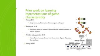
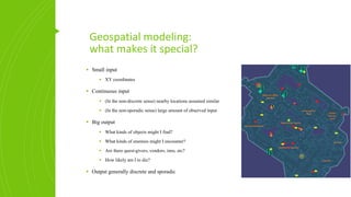
Discretization of Game
Space by Environment
Attributes
Alex Braylan and Risto Miikkulainen
The University of Texas at Austin
Introduction
▪ Games are becoming more complex
▪ Many characteristics of the game are not explicitly coded
▪ Need for learning high-level abstraction
▪ Non-player character (NPC) intelligence
▪ Analytics for player
▪ Analytics for designer
▪ Focus of this work is on geo-spatial environment
▪ What can be learned about xy coordinates
Prior work on learning
representations of game
characteristics
▪ Tomai 2018
▪ Graph structure of interactions between agents and objects
▪ Fulda et al 2018
▪ Interaction modes, or subsets of possible actions that are reasonable in
a given situation
▪ Winder and desJardins 2018
▪ Hierarchies of concepts formed from observations of game objects and
their attributes
▪ Many others
Geospatial modeling:
what makes it special?
▪ Small input
▪ XY coordinates
▪ Continuous input
▪ (In the non-discrete sense) nearby locations assumed similar
▪ (In the non-sporadic sense) large amount of observed input
▪ Big output
▪ What kinds of objects might I find?
▪ What kinds of enemies might I encounter?
▪ Are there quest-givers, vendors, inns, etc?
▪ How likely am I to die?
▪ Output generally discrete and sporadic
Geospatial modeling goals
▪ Usefulness
▪ Predictive power
▪ Interpretability
▪ Efficiency
▪ Memory requirement
▪ Compute time
Evaluation measures:
usefulness
▪ Predictive power
▪ How accurate are model’s predictions?
▪ Cross-entropy loss for categorical outcomes
▪ Interpretability
▪ NPC should communicate clearly with player
▪ Analytics should be transparent to designer
▪ Kernel (non-parametric) example:
“I am at coordinates (x, y), where by interpolation from observations at (x − 3,
y − 2), (x − 1, y + 1), (x + 2, y + 4) ... the probability of encountering a wolf
each minute is 0.12”
▪ Cluster (parametric) example:
“I am at coordinates (x, y), which are in biome type 7, where the probability of
encountering a wolf each minute is 0.12”
Evaluation measures:
efficiency
▪ Memory requirement
▪ Model output can be as complex as observation dimensionality
▪ Probability of encountering each type of enemy/object/etc
▪ Concrete measure in next slide
▪ Compute time
▪ Measure in seconds? CPU usage? Number of operations?
Biomes: simplifying complex
observation spaces
▪ Discretization of game space by environment attributes
▪ Map XY coordinates to biome IDs
▪ Biome IDs in observation probability table
▪ Store biome boundary definitions
▪ Memory efficiency measures
▪ Number of biomes
▪ Non-overlap, average fraction of nearest neighbors in geographical
space belonging to same biome
Biome 1 Biome 2 Biome 8
Wolf 0.05 0.36 0.00
Turtle 0.21 0.11 0.04
Shield 0.01 0.05 0.02
… … … …
Pirate 0.01 0.00 0.17
Learning biomes by clustering
▪ Geospatial input XY, observation attribute output Z
▪ Baselines:
K-means on XY K-means on Z
Ignored attributes Undefined boundaries
Learning biomes by clustering
▪
W
1 0 0
W
1 0 0
T
0 1 0
W
.5 .5 0
W
1 0 0
T
.5 .5 0
W: 0.87
T: 0.44
W
XY
proximit
y
check?
Learning biomes by clustering
▪ GCC/GAC define biomes according to characteristic inhabitants
▪ GCC/GAC enforce contiguity of biomes to minimize representation complexity
GCC GAC
Contiguous biomes Partially contiguous biomes
Evaluation of clustering
methods
Overlap Cross-entropy Seconds
K-means XY 1% 34.07 2.00
K-means Z 44% 5.33 1.17
GCC 2% 27.00 3.07
GAC 4% 27.83 6.87
▪ Modern multi-player first-person shooter game
▪ Three maps with 5000-18000 observations of 200-400 types of creatures
Least predictive
No compression
Slowest
Winner
Conclusion
▪ Geospatial modeling: an important part of a larger picture
▪ Models should be predictive, interpretable, compact, tractable
▪ Biome concept: maximize information, constrain complexity
▪ GCC & GAC: methods for learning biomes
▪ Future work:
▪ Integration with larger models
▪ Usefulness as explanatory variable should be dependent on other explanatory variables
▪ Z as residuals rather than observations?
▪ Defining boundaries
▪ Interpolating between biomes near boundaries
▪ Additional dimensions in space and time

Discretization of game space by environment attributes

  • 1.
    Discretization of Game Spaceby Environment Attributes Alex Braylan and Risto Miikkulainen The University of Texas at Austin
  • 2.
    Introduction ▪ Games arebecoming more complex ▪ Many characteristics of the game are not explicitly coded ▪ Need for learning high-level abstraction ▪ Non-player character (NPC) intelligence ▪ Analytics for player ▪ Analytics for designer ▪ Focus of this work is on geo-spatial environment ▪ What can be learned about xy coordinates
  • 3.
    Prior work onlearning representations of game characteristics ▪ Tomai 2018 ▪ Graph structure of interactions between agents and objects ▪ Fulda et al 2018 ▪ Interaction modes, or subsets of possible actions that are reasonable in a given situation ▪ Winder and desJardins 2018 ▪ Hierarchies of concepts formed from observations of game objects and their attributes ▪ Many others
  • 4.
    Geospatial modeling: what makesit special? ▪ Small input ▪ XY coordinates ▪ Continuous input ▪ (In the non-discrete sense) nearby locations assumed similar ▪ (In the non-sporadic sense) large amount of observed input ▪ Big output ▪ What kinds of objects might I find? ▪ What kinds of enemies might I encounter? ▪ Are there quest-givers, vendors, inns, etc? ▪ How likely am I to die? ▪ Output generally discrete and sporadic
  • 5.
    Geospatial modeling goals ▪Usefulness ▪ Predictive power ▪ Interpretability ▪ Efficiency ▪ Memory requirement ▪ Compute time
  • 6.
    Evaluation measures: usefulness ▪ Predictivepower ▪ How accurate are model’s predictions? ▪ Cross-entropy loss for categorical outcomes ▪ Interpretability ▪ NPC should communicate clearly with player ▪ Analytics should be transparent to designer ▪ Kernel (non-parametric) example: “I am at coordinates (x, y), where by interpolation from observations at (x − 3, y − 2), (x − 1, y + 1), (x + 2, y + 4) ... the probability of encountering a wolf each minute is 0.12” ▪ Cluster (parametric) example: “I am at coordinates (x, y), which are in biome type 7, where the probability of encountering a wolf each minute is 0.12”
  • 7.
    Evaluation measures: efficiency ▪ Memoryrequirement ▪ Model output can be as complex as observation dimensionality ▪ Probability of encountering each type of enemy/object/etc ▪ Concrete measure in next slide ▪ Compute time ▪ Measure in seconds? CPU usage? Number of operations?
  • 8.
    Biomes: simplifying complex observationspaces ▪ Discretization of game space by environment attributes ▪ Map XY coordinates to biome IDs ▪ Biome IDs in observation probability table ▪ Store biome boundary definitions ▪ Memory efficiency measures ▪ Number of biomes ▪ Non-overlap, average fraction of nearest neighbors in geographical space belonging to same biome Biome 1 Biome 2 Biome 8 Wolf 0.05 0.36 0.00 Turtle 0.21 0.11 0.04 Shield 0.01 0.05 0.02 … … … … Pirate 0.01 0.00 0.17
  • 9.
    Learning biomes byclustering ▪ Geospatial input XY, observation attribute output Z ▪ Baselines: K-means on XY K-means on Z Ignored attributes Undefined boundaries
  • 10.
    Learning biomes byclustering ▪ W 1 0 0 W 1 0 0 T 0 1 0 W .5 .5 0 W 1 0 0 T .5 .5 0 W: 0.87 T: 0.44 W XY proximit y check?
  • 11.
    Learning biomes byclustering ▪ GCC/GAC define biomes according to characteristic inhabitants ▪ GCC/GAC enforce contiguity of biomes to minimize representation complexity GCC GAC Contiguous biomes Partially contiguous biomes
  • 12.
    Evaluation of clustering methods OverlapCross-entropy Seconds K-means XY 1% 34.07 2.00 K-means Z 44% 5.33 1.17 GCC 2% 27.00 3.07 GAC 4% 27.83 6.87 ▪ Modern multi-player first-person shooter game ▪ Three maps with 5000-18000 observations of 200-400 types of creatures Least predictive No compression Slowest Winner
  • 13.
    Conclusion ▪ Geospatial modeling:an important part of a larger picture ▪ Models should be predictive, interpretable, compact, tractable ▪ Biome concept: maximize information, constrain complexity ▪ GCC & GAC: methods for learning biomes ▪ Future work: ▪ Integration with larger models ▪ Usefulness as explanatory variable should be dependent on other explanatory variables ▪ Z as residuals rather than observations? ▪ Defining boundaries ▪ Interpolating between biomes near boundaries ▪ Additional dimensions in space and time