MidtermReview.pdf
Statistics 411/511
Important Concepts and Tasks for the Midterm
(Not Necessarily in any Order)
Scope of Material for Midterm
The midterm will cover the material in Chapter 1 through Section 5.5, excluding Section 5.4
and the parts of Chapter 4 noted in item 4(a) below.
1. Two-sample t-test.
(a) Know assumptions, and assess their validity from graphical displays such as boxplots
and histograms.
(b) Given R output, write a brief (one or two sentences) statistical summary reporting results.
(c) Given summary statistics, write the t-statistic (this may entail calculating the pooled
standard deviation).
(d) Given summary statistics and a confidence level, write a confidence interval.
(e) Know how to find the degrees of freedom of the pooled standard deviation.
(f) Decide if a one-tailed or two-tailed test is most appropriate.
(g) Suggest a procedure to use when the equal-variance assumption is not met.
(h) Given R t.test() output, be able to tell if test was one- or two-sided and if equal
variance assumption was made or not.
2. Paired t-test
(a) Know when to use a paired t-test as opposed to a two-sample t-test.
(b) Know assumptions, and assess their validity from graphical displays such as boxplots
and histograms.
(c) Given R output, write a brief statistical summary reporting results.
(d) Given summary statistics, write the t-statistic.
(e) Given summary statistics and a confidence level, write a confidence interval.
(f) Decide if a one-tailed or two-tailed test is most appropriate.
3. Transformations
(a) Know when log or logit are appropriate transformations to consider.
(b) Back-transform and interpret results on the original scale after a log transformation.
4. Non-parametric Alternatives to t-tests
(a) We skipped the signed-rank test, so you should be familiar with the Wilcoxon rank-sum
test, Welch’s t-test, permutation/randomization tests, and the sign test. You can ignore
Levene’s test for the exam.
(b) Given a study, decide which procedures is/are appropriate.
1
(c) Given R output, write a brief statistical summary reporting results.
(d) Know the mean and standard deviation of the normal approximation to the sampling
distribution of the Wilcoxon rank-sum test statistic T or the sign test statistic K.
(e) Understand the principle behind a permutation/randomization test. (Technically, a per-
mutation test considers ALL random shufflings of the data, whereas a randomization test
just considers a large number of them. The test on the space shuttle O-ring in Section
4.3.1 is a permutation test. The test on the creativity study data in Section 1.3.2 is a
randomization test.)
5. One-way Analysis of Variance (ANOVA)
(a) Know assumptions and assess their validity from side-by-side boxplots or a residual plot.
(b) Given R anova() output, calculate the pooled standard deviation.
(c) Given R anova() output, find the degrees of freedom associated with a pooled standard
deviation.
(d) Given R anova ...
1. MidtermReview.pdf
Statistics 411/511
Important Concepts and Tasks for the Midterm
(Not Necessarily in any Order)
Scope of Material for Midterm
The midterm will cover the material in Chapter 1 through
Section 5.5, excluding Section 5.4
and the parts of Chapter 4 noted in item 4(a) below.
1. Two-sample t-test.
(a) Know assumptions, and assess their validity from graphical
displays such as boxplots
and histograms.
(b) Given R output, write a brief (one or two sentences)
statistical summary reporting results.
(c) Given summary statistics, write the t-statistic (this may
entail calculating the pooled
standard deviation).
(d) Given summary statistics and a confidence level, write a
confidence interval.
(e) Know how to find the degrees of freedom of the pooled
standard deviation.
(f) Decide if a one-tailed or two-tailed test is most appropriate.
2. (g) Suggest a procedure to use when the equal-variance
assumption is not met.
(h) Given R t.test() output, be able to tell if test was one- or
two-sided and if equal
variance assumption was made or not.
2. Paired t-test
(a) Know when to use a paired t-test as opposed to a two-sample
t-test.
(b) Know assumptions, and assess their validity from graphical
displays such as boxplots
and histograms.
(c) Given R output, write a brief statistical summary reporting
results.
(d) Given summary statistics, write the t-statistic.
(e) Given summary statistics and a confidence level, write a
confidence interval.
(f) Decide if a one-tailed or two-tailed test is most appropriate.
3. Transformations
(a) Know when log or logit are appropriate transformations to
consider.
(b) Back-transform and interpret results on the original scale
after a log transformation.
4. Non-parametric Alternatives to t-tests
3. (a) We skipped the signed-rank test, so you should be familiar
with the Wilcoxon rank-sum
test, Welch’s t-test, permutation/randomization tests, and the
sign test. You can ignore
Levene’s test for the exam.
(b) Given a study, decide which procedures is/are appropriate.
1
(c) Given R output, write a brief statistical summary reporting
results.
(d) Know the mean and standard deviation of the normal
approximation to the sampling
distribution of the Wilcoxon rank-sum test statistic T or the sign
test statistic K.
(e) Understand the principle behind a
permutation/randomization test. (Technically, a per-
mutation test considers ALL random shufflings of the data,
whereas a randomization test
just considers a large number of them. The test on the space
shuttle O-ring in Section
4.3.1 is a permutation test. The test on the creativity study data
in Section 1.3.2 is a
randomization test.)
5. One-way Analysis of Variance (ANOVA)
(a) Know assumptions and assess their validity from side-by-
side boxplots or a residual plot.
4. (b) Given R anova() output, calculate the pooled standard
deviation.
(c) Given R anova() output, find the degrees of freedom
associated with a pooled standard
deviation.
(d) Given R anova() output and sample means and sample sizes,
write a t-statistic to
compare two means.
(e) Given R anova() output and sample means and sample sizes,
write a confidence interval
to estimate the difference between two means.
(f) Write a brief statistical conclusion reporting results of
ANOVA F-test.
(g) Write a brief statistical conclusion reporting results of a t-
test comparing two means.
(h) Write a brief statistical conclusion reporting a confidence
interval for the difference be-
tween two means.
6. Understand Concepts
(a) Sampling distribution of a test statistic
(b) Confidence coverage
(c) Scope of inference (What population? Can we infer
causation?)
(d) Strength of evidence
5. (e) Practical significance vs. statistical significance
Recommendations for Midterm Preparation
1. The exam is closed book. You are allowed one one-sided 8.5
by 11-inch page of notes which
you’ll turn in with the exam (you’ll get it back).
2. Making summary notes is helpful. It’s a good way to review
and synthesize information from
class notes and textbook. Your one-sided page of notes may be
condensed from this.
3. Try to spread your review over several days rather than
cramming the night before the exam.
This will allow you to spend time focusing on particular topics
and get questions answered.
2
Recommendations for Taking the Midterm
1. Don’t rely too heavily on your one-sided page of notes. Aim
for a good understanding of the
material.
2. If a question requires a “brief statistical summary,” write no
more than necessary. The sum-
mary should answer the research question, include an
assessment of the strength of evidence,
and state the parameter(s) involved in the inference. Include the
p-value or confidence in-
terval. Go ahead and use abbreviations for long words. The
lecture notes contain several
6. “conclusions” which you can use as examples.
3. During the exam, don’t spend time calculating anything. For
example, suppose you are given
the following summary statistics for a sample of paired
differences: n = 12, Y = 4.1, and
sd = 1.57, and you are asked to calculate a 95% confidence
interval for the mean difference.
You’ll get full credit for 4.1±t11(0.975) ·1.57/
√
12. If you have time after finishing the exam,
you can go back and calculate (3.10247, 5.09753), but this not
necessary.
3
PracticeMidterm.pdf
Statistics 553 Name:
Practice Midterm
Midterm Instructions:
• This exam is closed-book. You may have one side of an
8.5×11-inch page of handwritten
notes, which you should turn in with your exam when finished.
• You may use a calculator but no device with internet access.
• You don’t actually have to carry out calculations. For
example, if you were asked for a 95%
confidence interval for a mean whose point estimate is 3, and
7. whose standard error is 1.5, and
with degrees of freedom is 5, you would receive full credit for
the answer 3 ± t5(0.975) · 1.5.
• The default α is 0.05.
• There are a total of 85 points possible.
• This is a 50-minute exam. Pace yourself. Do not spend so
much time on earlier problems
that you do not get to the later ones. Don’t write more than
necessary. It’s OK to abbreviate
words.
• Please be as clear and concise as possible.
Notes About this Practice Midterm:
• These problems are designed to give you an idea of the scope
and flavor of the type of problems
that may appear on the midterm. However, your review should
be comprehensive, not limited
to these problems.
• I recommend working through these problems on your own at
first, then working with each
other.
• The TAs will be prepared to answer questions about this
practice exam during lab on October
31 and November 1.
• The actual exam will be somewhat shorter than this practice
exam.
8. This page is intentionally blank.
1. Cuckoos are birds that lay their eggs in other birds’ nests. A
famous ecological study compared
lengths of cuckoo eggs found in nests of six different host
species. The research question is
to determine if cuckoo egg lengths differ among the host
species and to compare egg lengths
between host species. The R data frame eggs contains two
columns labeled Length and
Host (HS=hedge sparrow; MP=meadow pipit; PW=pied wagtail;
TP=tree pipit). Below are
boxplots and R commands and output from a one-way analysis
of variance of the data.
20
21
22
23
24
25
MP TP HS Robin PW Wren
Host
L
e
9. n
g
th
> head(eggs)
Host Length
1 MP 19.65
2 MP 20.05
3 MP 20.65
4 MP 20.85
5 MP 21.65
6 MP 21.65
> summary(eggs$Host) # Sample sizes
MP TP HS Robin PW Wren
16 15 14 16 15 15
> eggs.aov<-aov(Length~Host,data=eggs)
> anova(eggs.aov)
Analysis of Variance Table
Response: Length
Df Sum Sq Mean Sq F value Pr(>F)
10. Host 5 55.794 11.159 14.398 3.334e-10 ***
Residuals 85 65.876 0.775
> # Group sample means.
> with(eggs,unlist(lapply(split(Length,Host),mean)))
MP TP HS Robin PW Wren
21.50000 23.09000 23.12143 22.57500 22.90333 21.13000
3
(a) (4 points) State the null and alternative hypotheses tested by
F = 14.398 in the ANOVA
table above.
(b) (8 points) Do cuckoo egg lengths differ among host species?
Give a brief “statistical
conclusion.”
(c) (3 points) Can we conclude from the study that differing
host species causes differences
among cuckoo egg lengths? Explain briefly in one sentence.
(d) (8 points) Give a t-statistic to test for a difference in mean
length between eggs in tree
pipit’s vs. meadow pipit’s nests.
(e) (9 points) Give a 95% confidence interval for the difference
in mean length between eggs
in robin’s nests vs. wren’s nests.
11. 4
2. Water samples from random locations and depths were taken
from Silver Lake and Goose
Lake to compare chloride concentration of the water. Below are
side-by-side boxplots on the
original scale and on the log scale, as well as R output from a t-
test on the logged data.
10
20
30
Goose Silver
Lake
C
h
lo
ri
d
e
1.5
2.0
2.5
13. 2.720436 2.394761
(a) (11 points) Give a statistical conclusion answering the
question, “how do median chloride
concentrations differ between the two lakes?”
(b) (3 points) Answer in one sentence or less: What was the
purpose of the log transforma-
tion?
(c) (6 points) State the three assumptions needed for the t-test
and confidence interval to
be valid.
5
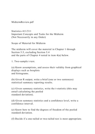
3. (5 points) The R data frame tornados contains yearly counts
of tornados in the United States
for the 66 years from 1950 to 2015. Suppose we want to know if
there are more tornados per
year after 1990 than before. The histogram below shows the
difference in average tornado
count between 1950 and 1989 compared to 1990 to 2015 for
10,000 random assignments of the
observed counts to the 66 years.
0
500
1000
1500
14. 2000
−4000 −2000 0 2000 4000
Difference
co
u
n
t
The actual difference in mean tornado counts between the
period 1950 to 1989 and the period
1990 to 2015 is -3106.038. Given the data, is it the plausible
that the yearly tornado count is
the same in the two periods? Explain briefly (no more than two
sentences).
6
4. The Department of Health and Social Services of the State of
New Mexico collected data on
nursing facilities in New Mexico in 1988 (data provided by
DASL, dasl.datadesk.com). Below
are histograms of federal expenditures per bed for rural and
non-rural nursing facilities. The
question of interest is if there is a difference between federal
expenditures at rural vs. non-rural
facilities.
0
1
16. 0 5 10 15 20
Federal Expenditures per Bed ($)
co
u
n
t
Below are the first few rows of the data set, sample size
information, and R output from a
Wilcoxon rank-sum test.
> head(Ndata)
Fexp.bed Rural
1 4.574428 Nonrural
2 11.967546 Rural
3 1.962388 Nonrural
4 1.890955 Nonrural
5 1.927711 Nonrural
6 14.476615 Rural
> summary(Ndata$Rural)
Nonrural Rural
18 34
> wilcox.test(Fexp.bed~Rural,data=Ndata)
17. Wilcoxon rank sum test
data: Fexp.bed by Rural
W = 320, p-value = 0.7971
alternative hypothesis: true location shift is not equal to 0
> # Find the mean and standard deviation of the ranked data.
> r.Fexp.bed <- rank(Fexp.bed)
> mean(r.Fexp.bed)
[1] 26.5
> sd(r.Fexp.bed)
[1] 15.15476
7
(a) (4 points) State the null and alternative hypotheses tested by
the statistic W = 320 in
the above output.
(b) (6 points) State the mean and standard deviation of the
normal approximation to the
sampling distribution of the Wilcoxon rank-sum test statistic T
for these data. (Recall
that the textbook uses test statistic T whereas R uses test
statistic W, and W = T −
n1(n1+1)
18. 2
where n1 is the sample size from the first group.)
(c) (8 points) Give a statistical conclusion answering the
research question.
8
5. (10 points) For each of the studies described below, select all
statistical procedures that would
be appropriate if their assumptions were met. “Appropriate”
here means that you could make
a case for using the procedure by verifying the reasonableness
of the assumptions.
(a) Researchers performed an experiment to test whether
directed reading activities in the
classroom help elementary school students improve aspects of
their reading ability. A
treatment class of 21 third-grade students participated in these
activities for eight weeks,
and a control class of 23 third-graders followed the same
curriculum without the activities.
After the eight-week period, students in both classes took a
reading test, and their test
scores were recorded.
Circle all your choices:
two-sample t-test Wilcoxon rank-sum test
paired t-test sign test
Welch’s t-test one-way ANOVA
19. (b) A study was performed to compare germination of seeds
treated with fungicide to un-
treated seeds. Sixteen one-meter square garden plots were used.
Half of each plot was
seeded with 100 treated seeds and half with 100 untreated seeds.
The number of seedlings
from each half of a plot was recorded for each plot.
Circle all your choices:
two-sample t-test Wilcoxon rank-sum test
paired t-test sign test
Welch’s t-test one-way ANOVA
(c) Food scientists conducted an experiment comparing five
different packaging methods
for cheese. They randomly assigned 10 eight-ounce blocks of
cheese to each of the five
methods. The 50 blocks of cheese were stored for six months,
then each block was tested
for bacteria. The number of bacteria on each block was recorded
Circle all your choices:
two-sample t-test Wilcoxon rank-sum test
paired t-test sign test
Welch’s t-test one-way ANOVA
9
PracticeFinal.pdf
Statistics 553 Name:
Practice Final
20. Instructions:
• This exam is closed-book. You may have both sides of an
8.5×11-inch page of notes, which
you should turn in with your exam when finished.
• You may use a calculator but no device with internet access.
• You don’t actually have to carry out calculations. For
example, if you were asked for a 95%
confidence interval for a mean whose point estimate is 3, with
standard error 1.5, degrees of
freedom 5, you would receive full credit for the answer 3 ±
t5(0.975) · 1.5.
• The default α is 0.05.
• There are a total of 95 points possible.
• This is a 110-minute exam. Pace yourself. Do not spend so
much time on earlier problems
that you do not get to the later ones. Don’t write more than
necessary. It’s OK to abbreviate
words.
• Please be as clear and concise as possible.
Notes About this Practice Exam:
• These problems are designed to give you an idea of the scope
and flavor of the type of problems
that may appear on the final. However, your review should be
comprehensive, not limited to
these problems. Review the labs, homework, midterm, and
practice midterm.
21. • I recommend working through these problems on your own at
first, then working with each
other.
• The actual exam will be somewhat shorter than this practice
exam.
This page is intentionally blank.
1. Recall the cuckoo egg length study from the practice
midterm. The study compared lengths
of cuckoo eggs among six different host species. The research
question is to determine if
cuckoo egg lengths differ among the host species and to
compare egg lengths among host
species (HS=hedge sparrow; MP=meadow pipit; PW=pied
wagtail; TP=tree pipit). Below
is R output from a one-way analysis of variance of the data.
Analysis of Variance Table
Response: Length
Df Sum Sq Mean Sq F value Pr(>F)
Host 5 55.794 11.159 14.398 3.334e-10 ***
Residuals 85 65.876 0.775
Tables of means
22. Host
HS MP PW Robin TP Wren
23.12 21.5 22.90 22.57 23.09 21.13
rep 14.00 16.0 15.00 16.00 15.00 15.00
(a) (8 points) Suppose the pairwise comparisons of interest are
between mean length of eggs
in hedge sparrow’s vs. meadow pipit’s nests and between hedge
sparrow’s vs. pied
wagtail’s nests Write 95% Bonferroni confidence intervals for
these comparisons.
(b) (4 points) Write the Scheffé multiplier you would calculate
for Scheffé versions of the two
confidence intervals in (a).
(c) (2 points) If the comparisons of interest were between all
pairs of host species, what
multiple comparison procedure would you use?
(d) (4 points) Using the R output above, give the residual sum
of squares and degrees of
freedom for the equal means model.
3
2. In a study on mercury levels in fish, water samples and fish
were collected from 53 lakes in
Florida. In the data set, Avg.Mercury is the average mercury
concentration (parts per million)
in muscle tissue of the fish sampled from the lake. Alkalinity is
23. mg/L of calcium chloride in
the water sample collected from the lake. Below is a scatterplot
of log(Avg.Mercury) vs.
Alkalinity with fitted regression line and confidence band.
−3
−2
−1
0
0 50 100
Alkalinity
lo
g
(A
vg
.M
e
rc
u
ry
)
R output from the regression is below.
> lakes.lm<-lm(log(Avg.Mercury)~Alkalinity)
> summary(lakes.lm)
24. Call:
lm(formula = log(Avg.Mercury) ~ Alkalinity)
Residuals:
Min 1Q Median 3Q Max
-2.06553 -0.27948 0.08225 0.29231 1.79197
Coefficients:
Estimate Std. Error t value Pr(>|t|)
(Intercept) -0.321099 0.114715 -2.799 0.00722 **
Alkalinity -0.015703 0.002152 -7.295 1.86e-09 ***
---
Signif. codes: 0 *** 0.001 ** 0.01 * 0.05 . 0.1 1
Residual standard error: 0.593 on 51 degrees of freedom
Multiple R-squared: 0.5107,Adjusted R-squared: 0.5011
F-statistic: 53.22 on 1 and 51 DF, p-value: 1.859e-09
4
(a) (7 points) Write a 95% confidence interval for the intercept
parameter β0 in the regression
model.
25. (b) (11 points) A 95% confidence interval for β1 is
(−0.02,−0.01). Write a statistical con-
clusion reporting this result.
(c) (5 points) Use the R predict() output below to give a
confidence interval for the median
average mercury concentration expected in a lake with an
alkalinity of 100 mg/L of
calcium chloride.
>
predict(lakes.lm,data.frame(Alkalinity=100),interval="confiden
ce",se.fit=TRUE)
$fit
fit lwr upr
1 -1.891373 -2.206977 -1.57577
$se.fit
[1] 0.1572056
$df
[1] 51
$residual.scale
[1] 0.5929642
(d) (6 points) Use the R predict() output above to write a 95%
prediction interval for
the average mercury concentration of fish in a lake with an
26. alkalinity of 100 mg/L of
calcium chloride.
This problem is continued on the next page.
5
(e) (4 points) State the full and reduced models tested by the F-
statistic 53.224 in the output
below.
> anova(lakes.lm)
Analysis of Variance Table
Response: log(Avg.Mercury)
Df Sum Sq Mean Sq F value Pr(>F)
Alkalinity 1 18.714 18.7138 53.224 1.859e-09 ***
Residuals 51 17.932 0.3516
(f) (4 points) A residual plot and normal Q-Q plot are shown
below. For each of the two
plots, state the assumption it is used to check and your
assessment of the plausibility of
the assumption based on the plot.
−2.0 −1.5 −1.0 −0.5
−
2
29. ls
lm(log(Avg.Mercury) ~ Alkalinity)
Normal Q−Q
38
40
3
6
3. A study was conducted to compare waste between two
suppliers of a Levi-Strauss clothing
manufacturing plant. The firm’s quality control department
collects weekly data on percent-
age waste relative to what can be achieved by computer layouts
of patterns on cloth. It is
possible to have negative values, which indicate that the plant
employees beat the computer
in controlling waste. Below is a side-by-side boxplot of waste
for the two suppliers (plants)
and R output from a Wilcoxon rank-sum test.
0
25
50
Plant1 Plant2
Plant
30. W
a
st
e
>
wilcox.test(Waste~Plant,data=waste,exact=FALSE,correct=FAL
SE)
Wilcoxon rank sum test
data: Waste by Plant
W = 131.5, p-value = 0.009484
alternative hypothesis: true location shift is not equal to 0
(a) (4 points) State the null hypothesis tested by the statistic W
= 131.5 in the above
output.
(b) (7 points) Write a statistical conclusion reporting the result
of the rank-sum test.
(c) (3 points) Would a two-sample t-test be an appropriate
procedure for these data? Why
or why not? Answer in one sentence or less.
7
4. A study was performed to compare germination of seeds
treated with fungicide to untreated
31. seeds. Sixteen one-meter square garden plots were used. Half of
each plot was seeded with 100
treated seeds and half with 100 untreated seeds. The variable
diff is the difference between
the number of seedlings on the treated half and the number on
the untreated half (i.e. when
diff > 0, the treated half had more seedlings).
(a) (7 points) Below is R output from a t-test on the differences.
Write a statistical conclusion
reporting the results.
> t.test(diff,alternative="greater")
One Sample t-test
data: diff
t = 2.8652, df = 15, p-value = 0.005898
alternative hypothesis: true mean is greater than 0
95 percent confidence interval:
5.798254 Inf
sample estimates:
mean of x
14.9375
(b) (6 points) The sample standard deviation of the differences
is 20.85336. Write a two-sided
confidence interval for the mean difference µ.
32. (c) (2 points) State the p-value of a two-sided test of µ = 0.
(d) (3 points) Would a two-sample t-test be a reasonable
analysis for these data? Why or
why not? Answer in one sentence or less.
8
5. For this question, assume that a parametric procedure is one
that requires an assumption of
normality, whereas a nonparametric procedure does not. For
each of the studies described,
state one parametric and one nonparametric procedure that you
would consider for analysing
the data.
(a) (4 points) A city conducts a study comparing two types of
traffic control at intersections
to identify the type of intersection associated with fewer
accidents. City engineers identify
12 intersections of the first type, and 10 of the second type. The
number of accidents at
each of the 22 intersections for the past five years is recorded.
Parametric procedure:
Nonparametric procedure:
(b) (4 points) An insurance company suspects an automobile
repair garage of inflating the
charge of repairing cars after they’ve been involved in an
accident. Ten cars were taken
to the garage for a cost estimate. The same ten cars were taken
to another garage for
33. an estimate. The research question is if the cost estimates from
the suspect garage are
higher than from the other garage.
Parametric procedure:
Nonparametric procedure:
9
FinalReview.pdf
Statistics 411/511
Important Concepts and Tasks for the Final
(Not Necessarily in any Order)
The final is comprehensive and will cover the material in
Chapter 1 through Chapter 8 with
approximately equal emphasis on the material before and after
the midterm. Use the review outline
posted before the midterm as well as this one. We will have one
hour and fifty minutes for the final,
more than twice what we had for the midterm. The final will be
approximately 15% longer than
the midterm.
1. One-way ANOVA
(a) Be able to state the null and alternative hypotheses for the
ANOVA F-test.
(b) Given R output, be able to write a summary statement
describing the results of the
ANOVA F-test.
34. (c) Know the assumptions for the ANOVA F-test.
(d) Given R output, be able to write a confidence interval for
the difference between two
population means. Also be able to write a summary statement
reporting this interval.
(e) Know what the residuals are and how we use them to assess
assumptions.
(f) Given a plot of residuals vs. fitted values, comment on the
validity of the assumptions.
2. Inference About Linear Combinations of Means γ = C1µ1 + .
. .CIµI
(a) Given a research question, be able to determine the
coefficients C1, . . . ,CI .
(b) Given R output, be able to write a point estimate g and a
standard error SE(g).
(c) Given R output, be able to write a confidence interval for γ.
(d) Be able to report a confidence interval in a statistical
summary.
3. Extra Sum of Squares F-Tests
(a) Know in principle what the residual sum of squares is and
how to get it from the R
anova() output.
(b) Given a model and sample size, calculate residual degrees of
freedom.
35. (c) Find residual degrees of freedom on an ANOVA table or in
R output.
(d) For any two of the following models, decide which is the
full model and which is the
reduced model: separate means, equal means, simple linear
regression. Be able to state
the null hypothesis tested by the extra sum of squares F-test.
(e) Given R output, calculate an F-statistic for an extra sum of
squares test by hand.
4. Multiple Comparisons
(a) Understand the simultaneous inference problem.
(b) Know how to calculate confidence intervals using the four
multiple comparison procedures
covered, given appropriate R output. The four procedures are
Tukey-Kramer, Scheffé,
Dunnett, and Bonferroni.
1
(c) Know the appropriate use and limitations of the four
multiple comparison procedures.
5. Simple Linear Regression
(a) Know the assumptions for linear regression.
(b) Given R output, be able to write a confidence interval for β0
or β1.
36. (c) Write a statistical conclusion reporting an estimate of β1
when either the response or
predictor variable (or neither) have been log-transformed. (For
the ST 411/511 final, do
not worry about the case where both response and predictor
have been logged.)
(d) Decide if a prediction interval or a confidence interval is
most appropriate.
(e) Given R predict() output, write a prediction or confidence
interval.
(f) Write a statistical conclusion reporting a confidence interval
for β0.
(g) Assess assumptions from a residual plot or a normal Q-Q
plot.
(h) Given appropriate R predict() output, write a calibration
prediction or confidence
interval for X
̂ , the value of explanatory variable X associated
with a specified value of
the response Y0.
Recommendations
The same recommendations apply to the final as to the midterm.
As on the midterm, you will
not need to do any calculations on the final.
2