Linear regression

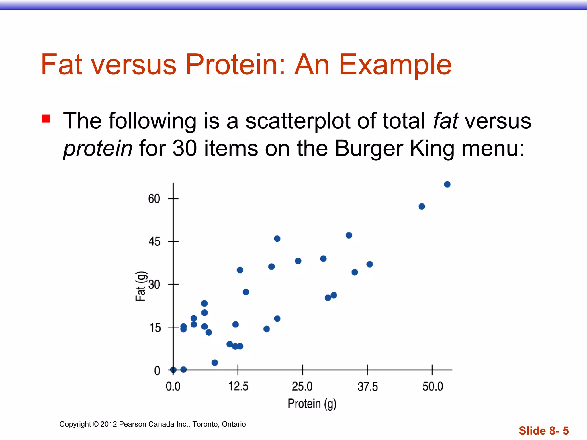
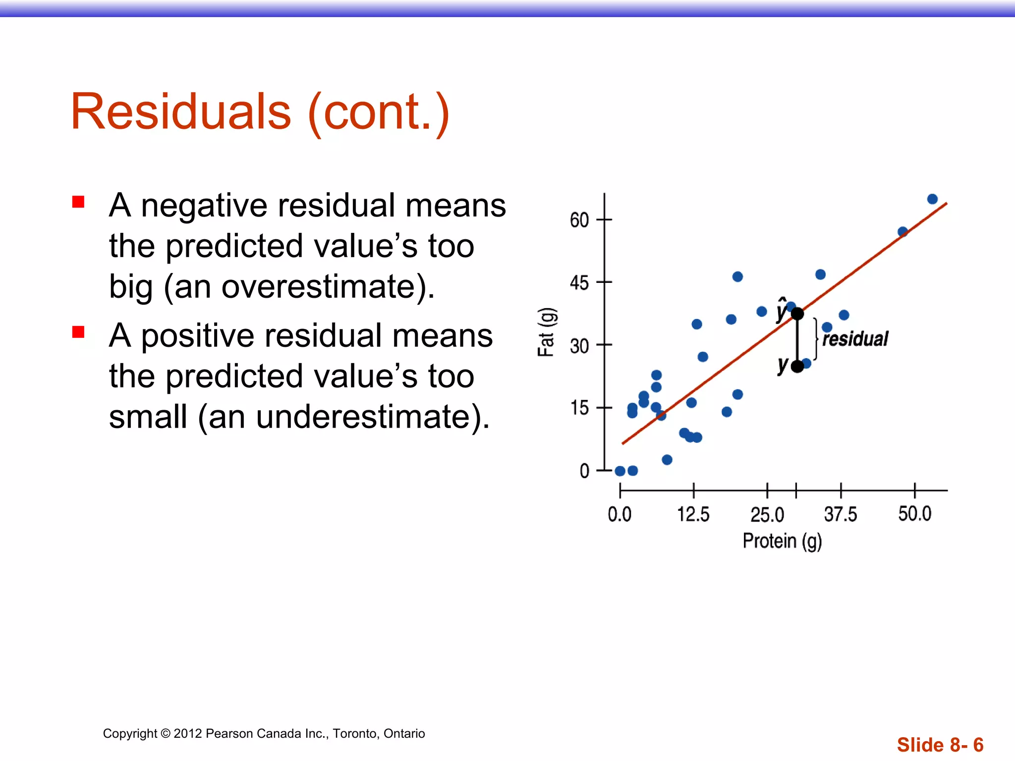
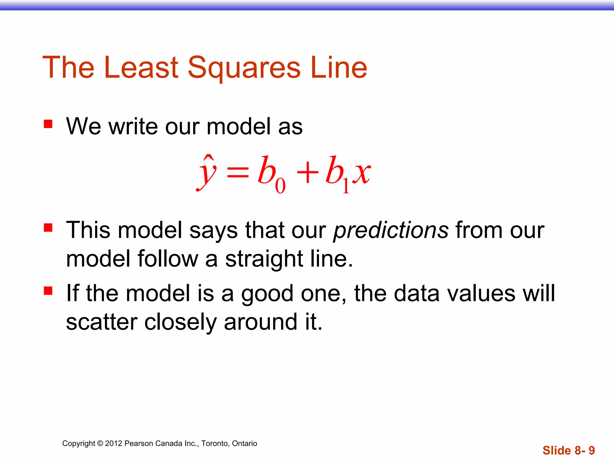
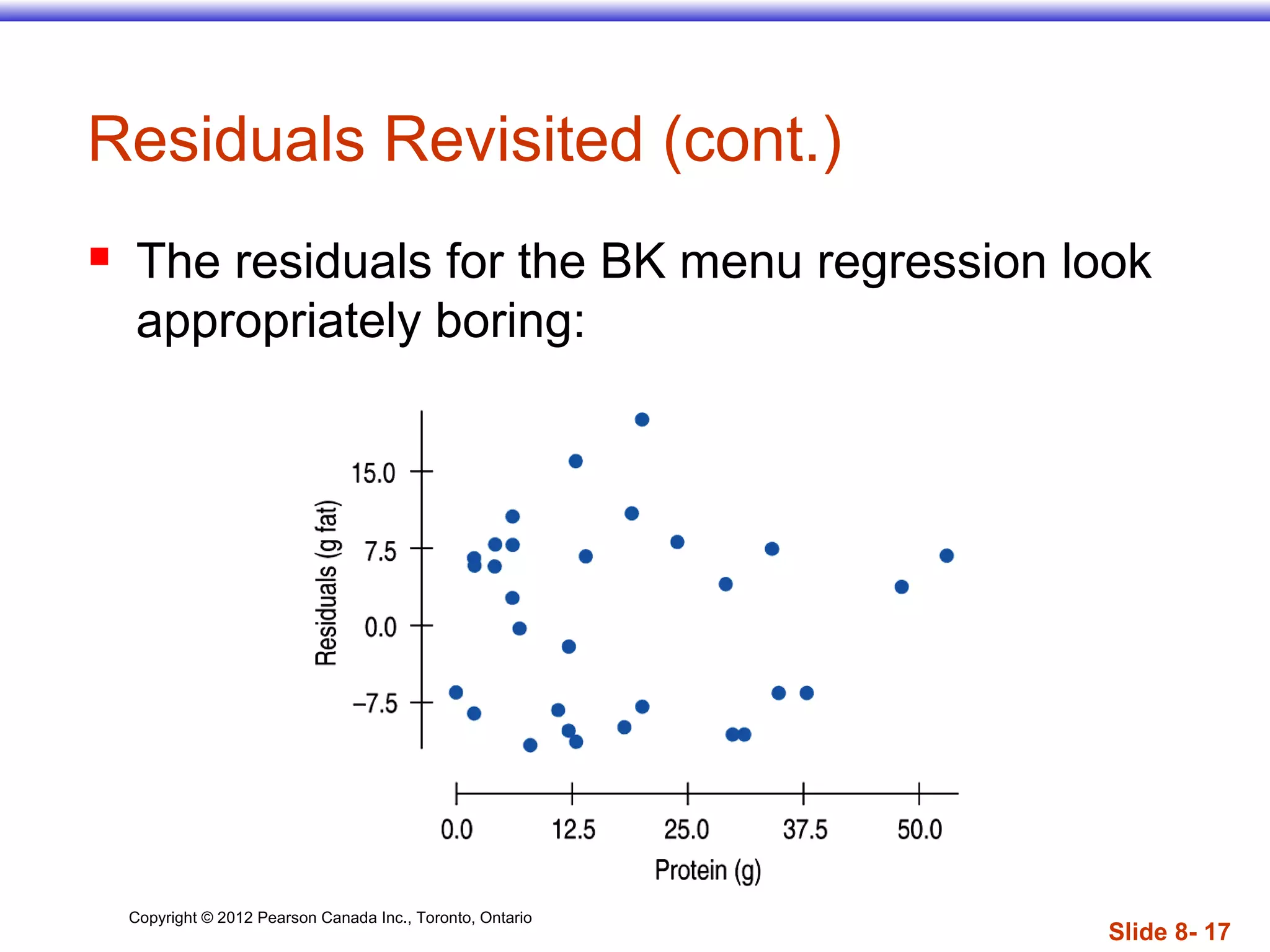
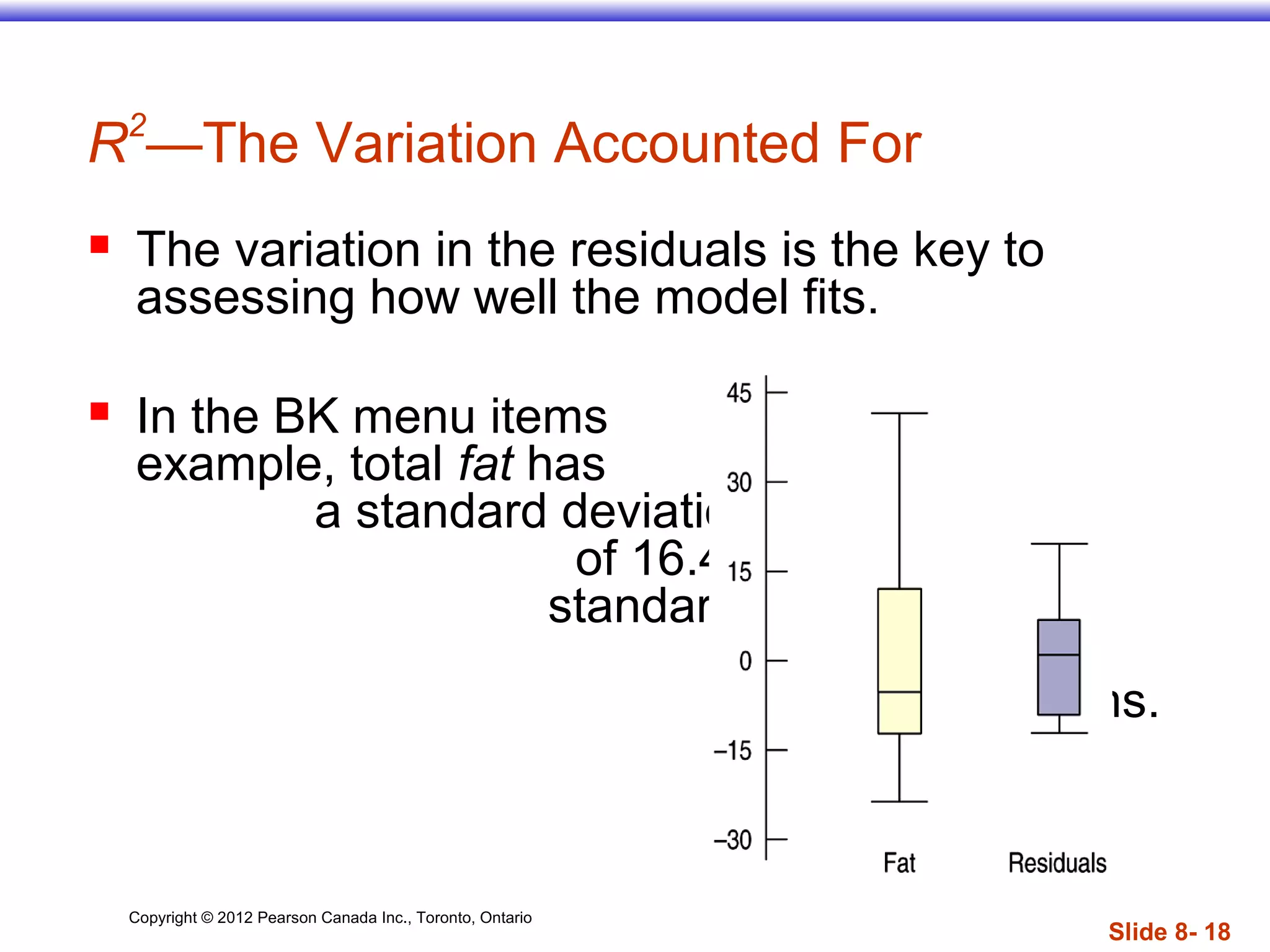
Copyright © 2012 Pearson Canada Inc., Toronto, Ontario
Slide 8- 1
The Linear Model
 Correlation says “There seems to be a linear
association between these two variables,” but it
doesn’t tell what that association is.
 We can say more about the linear relationship
between two quantitative variables with a model.
 A model simplifies reality to help us understand
underlying patterns and relationships.

Slide 8- 2
The Linear Model (cont.)
 The linear model is just an equation of a straight
line through the data.
 The points in the scatterplot don’t all line up,
but a straight line can summarize the general
pattern.
 The linear model can help us understand how
the values are associated.

Slide 8- 3
Residuals
 The model won’t be perfect, regardless of the line
we draw.
 Some points will be above the line and some will
be below.
 The estimate made from a model is the predicted
value (denoted as ).ˆy

Slide 8- 4
Residuals (cont.)
 The difference between the observed value and
its associated predicted value is called the
residual.
 To find the residuals, we always subtract the
predicted value from the observed one:
ˆresidual observed predicted y y= − = −

Slide 8- 5
Fat versus Protein: An Example
 The following is a scatterplot of total fat versus
protein for 30 items on the Burger King menu:

Slide 8- 6
Residuals (cont.)
 A negative residual means
the predicted value’s too
big (an overestimate).
 A positive residual means
the predicted value’s too
small (an underestimate).

Why do we need them?
Regression models have many
applications in industry and science.
Regression models can predict future trends, like
population growth.
Regression models can be used to estimate costs
and profits for businesses.
Regression models can help medical care
professionals determine how much medication to
prescribe for their patients.

Slide 8- 8
“Best Fit” Means Least Squares
 Some residuals are positive, others are negative,
and, on average, they cancel each other out.
 So, we can’t assess how well the line fits by
adding up all the residuals.
 Similar to what we did with deviations, we square
the residuals and add the squares.
 The smaller the sum, the better the fit.
 The line of best fit is the line for which the sum of
the squared residuals is smallest.

Slide 8- 9
The Least Squares Line
 We write our model as
 This model says that our predictions from our
model follow a straight line.
 If the model is a good one, the data values will
scatter closely around it.
0 1
ˆy b b x= +

Slide 8- 10
The Least Squares Line (cont.)
 In our model, we have a slope (b1):
 The slope is built from the correlation and the
standard deviations:
 Our slope is always in units of y per unit of x.
1
y
x
s
b r
s
=

Copyright © 2012 Pearson Canada Inc., Toronto, Ontario 11
The Least Squares Equation
 The formulas for b1 and b0 are:
algebraic equivalent:
∑ ∑
∑ ∑ ∑
−
−
=
n
x
x
n
yx
xy
b 2
2
1
)(
∑
∑
−
−−
= 21
)(
))((
xx
yyxx
b
xbyb 10 −=
and

Slide 8- 12
Fat versus Protein: An Example
 The regression line for the
Burger King data fits the
data well:
 The equation is
 The predicted fat
content for a BK Broiler
chicken sandwich is
6.8 + 0.97(30) = 35.9
grams of fat.

Slide 8- 13
The Least Squares Line (cont.)
 Since regression and correlation are closely
related, we need to check the same conditions for
regressions as we did for correlations:
 Quantitative Variables Condition
 Straight Enough Condition
 Outlier Condition

Slide 8- 14
How Big Can Predicted Values Get?
 r cannot be bigger than 1 (in absolute value),
so each predicted y tends to be closer to its mean
(in standard deviations) than its corresponding
x was.
 This property of the linear model is called
regression to the mean; the line is called the
regression line.

Slide 8- 15
Residuals Revisited
 The linear model assumes that the relationship
between the two variables is a perfect straight
line. The residuals are the part of the data that
hasn’t been modeled.
Data = Model + Residual
or (equivalently)
Residual = Data – Model
Or, in symbols,
ˆe y y= −

Slide 8- 16
Residuals Revisited (cont.)
 Residuals help us to see whether the model
makes sense.
 When a regression model is appropriate, nothing
interesting should be left behind.
 After we fit a regression model, we usually plot
the residuals in the hope of finding…nothing.

Slide 8- 17
Residuals Revisited (cont.)
 The residuals for the BK menu regression look
appropriately boring:

Slide 8- 18
R2
—The Variation Accounted For
 The variation in the residuals is the key to
assessing how well the model fits.
 In the BK menu items
example, total fat has
a standard deviation
of 16.4 grams. The
standard deviation
of the residuals
is 9.2 grams.

Slide 8- 19
R2
—The Variation Accounted For (cont.)
 If the correlation were 1.0 and the model
predicted the fat values perfectly, the residuals
would all be zero and have no variation.
 As it is, the correlation is 0.83—not perfection.
 However, we did see that the model residuals
had less variation than total fat alone.
 We can determine how much of the variation is
accounted for by the model and how much is left
in the residuals.

Slide 8- 20
R2
 The squared correlation, r2
, gives the fraction of
the data’s variance accounted for by the model.
 Thus, 1– r2
is the fraction of the original variance
left in the residuals.
 For the BK model, r2
= 0.832
= 0.69, so 31% of the
variability in total fat has been left in the
residuals.

Slide 8- 21
R2
 All regression analyses include this statistic,
although by tradition, it is written R2
(pronounced
“R-squared”). An R2
of 0 means that none of the
variance in the data is in the model; all of it is still
in the residuals.
 When interpreting a regression model you need
to Tell what R2
means.
 In the BK example, 69% of the variation in total
fat is accounted for by the model.

Slide 8- 22
How Big Should R2
Be?
 R2
is always between 0% and 100%. What makes
a “good” R2
value depends on the kind of data
you are analyzing and on what you want to do
with it.
 The standard deviation of the residuals can give
us more information about the usefulness of the
regression by telling us how much scatter there is
around the line.

Slide 8- 23
Regressions Assumptions and Conditions (cont.)
 It’s a good idea to check linearity again after
computing the regression when we can examine
the residuals.
 You should also check for outliers, which could
change the regression.
 If the data seem to clump or cluster in the
scatterplot, that could be a sign of trouble worth
looking into further.

Slide 8- 24
 If the scatterplot is not straight enough, stop here.
 You can’t use a linear model for any two
variables, even if they are related.
 They must have a linear association or the
model won’t mean a thing.
 Some nonlinear relationships can be saved by re-
expressing the data to make the scatterplot more
linear.
Regressions Assumptions and Conditions (cont.)

Slide 8- 25
What Can Go Wrong?
 Don’t fit a straight line to a nonlinear relationship.
 Beware extraordinary points (y-values that stand off from
the linear pattern or extreme x-values).
 Don’t extrapolate beyond the data—the linear model may
no longer hold outside of the range of the data.
 Don’t infer that x causes y just because there is a good
linear model for their relationship—association is not
causation.
 Don’t choose a model based on R2
alone.

Linear regression

More Related Content

Similar to Linear regression

More from suncil0071

Recently uploaded

Linear regression