Download 23115 cheat sheet completely free + more videos and notes: http://goo.gl/DdkL9P

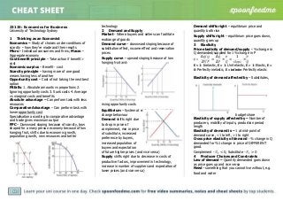
1. 23115: Economics for Business
University of Technology Sydney
1 Thinking as an Economist
Economics – Study of choices under conditions of
scarcity – how they’re made and their results
Micro - Individual consumers and firms; Macro -
Aggregate economy
Cost benefit principle – Take action if benefit >
cost
Economic surplus – Benefit - cost
Scarcity principle – having more of one good
means having less of another
Opportunity cost – Cost of not taking the next best
option
Pitfalls: 1. Absolute amounts vs proportions 2.
Ignoring opportunity costs 3. Sunk costs 4. Average
vs marginal costs and benefits
Absolute advantage – Can perform task with less
resources
Comparative Advantage – Can perform task with
lower opportunity cost
Specialisation according to comparative advantage
and trade gives maximum output
PPC – Downward sloping because of scarcity, bow
shaped for a many person economy because of low
hanging fruit, shifts due to economic growth,
population growth, new resources and better
technology
2 Demand and Supply
Market - Where buyers and sellers can facilitate
exchange of goods
Demand curve – downward sloping because of
substitution effect, income effect and reservation
prices
Supply curve – upward sloping because of low
hanging fruit and
rising opportunity costs
Equilibrium – System at rest, nobody wants to
change behaviour
Demand shifts right due
to drop in price of
complement, rise in price
of substitute, increased
preference by buyers,
increased population of
buyers and expectation
of future higher prices (and vice versa)
Supply shifts right due to decrease in costs of
productive factors, improvement in technology,
increase in number of suppliers and expectation of
lower prices (and vice versa)
Demand shifts right – equilibrium price and
quantity both rise
Supply shifts right – equilibrium price goes down,
quantity goes up
3 Elasticity
Price elasticity of demand/supply - % change in
Q demanded/supplied for 1% change in P
=
∆ /
∆ /
=
∆
∆
× =
1
×
E < 1: Inelastic, E = 1: Unit elastic, E > 1: Elastic, E =
0: Perfectly inelastic, E = infinite: Perfectly elastic
Elasticity of demand affected by – Substitutes,
budget share
Elasticity of supply affected by – Number of
producers, mobility of inputs, production period
length
Elasticity of demand is – 1 at mid-point of
demand curve, <1 to left, >1 to right
Cross price elasticity of demand - % change in Q
demanded for %1 change in price of DIFFERENT
good.
Complement - < 0, Substitute - > 0
4 Producer Choices and Constraints
Law of demand – Quantity demanded goes down
as price goes up and vice versa
Need - something that you cannot live without, e.g.
food and water

2. Want - something you would like to have, but don’t
need, e.g. ribs. Demand represents wants
Law of diminishing marginal utility – additional
utility (benefit) of consuming an extra unit of a good
decreases with consumption
Rational spending rule – Spend until marginal
benefit = marginal cost
Law of Supply – Quantity supplied goes up as price
goes up and vice versa
Constructing Market demand and supply
curves – Add HORIZONTALLY
Perfect competition – Profit maximizing firms,
price takers, identical products, many buyers and
sellers, no barriers to entry or exit, well informed
buyers and sellers
Fixed costs – Don’t change
Variable costs – Change with production
Profit
maximization
rule – Price =
Marginal cost
Consumer and Producer surplus – Difference
between reservation price and price paid
5 Efficiency
Pareto
improvement –
Somebody is made
better off and
nobody is made
worse off
Pareto efficiency
– No more Pareto
improvements can
occur
Economic surplus in a market is maximized
when exchange occurs at the equilibrium price
Causes of deadweight loss – Price floors, price
ceilings, price subsidies, taxes
6 The Invisible Hand
Accounting profit – Revenue - explicit costs;
Economic profit – Accounting profit – opp. costs
Normal profit – Economic profit = 0 (Normal profit
is opportunity cost)
Invisible Hand theory – Buyers and sellers acting
selfishly and independently will result in socially
optimal allocation of resources and best outcome for
everyone
Forms of market efficiency
Weak Semi-strong Strong
Info reflected
in share price
Private Public Both
7 Monopoly, Monopolistic Competition and
Price Discrimination
Price taker – Firm will lose all sales if price higher
than market price. Demand curve is perfectly elastic.
Price setter – Firm can change price and not lose all
sales. Demand curve is downward sloping.
Three types of imperfect competition
Pure
monopoly
Oligopoly Monopolistic
competition
Single firm Few large
firms
Many firms with
differentiated
products
Sydney
airport
ANZ, CBA,
Westpac, NAB
Restaurants
Monopolies arise from – Exclusive access to
resources, government, economies of scale
Economies of scale – Average cost goes down as
production goes up. Average cost = (Fixed costs +
Variable costs) / Quantity; FC/Q goes down with Q,
VC/Q goes up (diminishing marginal returns).
Diseconomies of scale when average starts to rise
Monopolist’s profit
maximization rule – =

3. MR NOT Price; higher production means price must
be lowered to get sufficient demand; MR decreasing.
Price discrimination – charging different prices to
different buyers for same good
Perfect price discrimination – Charging
customers their exact reservation price
8 Oligopoly and Game Theory
A game has – players, strategies, payoffs
Dominant strategy – Gives highest payoff no
matter what other players choose
Nash equilibrium – Every player has highest payoff
given other player choices
Prisoner’s dilemma – Every player has dominant
strategy but they are all better off if all choose
dominated strategy
The oligopoly prisoner’s dilemma – Can agree to
set price at monopolist profit maximizing level (form
a cartel), but each has incentive to lower price to
gain market share. Price war leads to lower profits for
all.
9 Externalities and Common Resources
Externality – Cost (negative) or benefit (positive) to
somebody not involved in activity. Causes
deadweight loss (see graph)
Coase theorem – Problems with externalities are
solved by people negotiating prices of property rights
IF transaction costs are low
Government solutions to externalities –
Regulations, market-based instruments (taxes,
subsidies, cap and trade)
Common resources – Resources that it is difficult
to exclude people from using (e.g. a lake)
Open access – When anybody can use a common
resource
Tragedy of the commons – Common resources
with open access are used by more and more people
until total surplus drops to zero
Positional externalities - a change in one person’s
performance changes the expected reward of another
in situations where reward depends on relative
performance
Positional arms race – Positional externalities lead
to series of continually offsetting investments in
performance by 2 players, e.g. use of performance
enhancing drugs in professional sport
10 Public Goods
Rivalry – Consumption of good by one person
means there is less available for another
Excludability – People can be prevented from using a
good if they don’t pay
Rivalrous Non-rivalrous
Excludable Private goods Collective goods
Non-excludable Common goods Public goods
Free rider problem – people value public goods but
avoid paying for them because they know they can’t
be excluded. Public goods don’t get sufficient funding
if too many people do this. Solved by taxes.
Head tax – Everybody pays same amount
Regressive tax – Proportion of income paid in taxes
declines as income rises (head tax is regressive)
Proportional income tax - all taxpayers pay the
same proportion of their incomes in taxes
Progressive tax - Proportion of income paid in
taxes rises as income rises
11 GDP, Unemployment and the Circular Flow
of Income
Macroeconomic goals - Rising living standards,
avoidance of expansions/contractions, stable
inflation, manageable debt, balance of
consumption/saving.
GDP – Market value of final goods and services
produced in a country during a given period of time
Production method – Sum market values of final
goods/services produced domestically
Expenditure method – Sum amounts spent on final
goods/services produced domestically
Income method – Sum revenue distributed from
sale of final goods/services produced domestically
Nominal GDP calculated with prices for that year
Real GDP calculated with prices from a base year

4. Real GDP generally indicates economic well-being but
ignores distribution of wealth, leisure, etc
CPI – Cost of a basket of goods in current year
divided by cost of basket in base year
Inflation - =
Inflation costs – Shoe-leather costs, noise in price
system, distortions of tax system, unexpected
redistribution of wealth, interference with long-run
planning and menu costs
= −
=
100
ℎ= −
∆ ℎ= + −
Saving Lifecycle Precautionar
y
Bequest
Reason Life goals Emergencies Inheritance
Real interest rate and inflation – 1 + =
Aggregate saving – = − −
Private saving – = − −
Public saving – = −
Investment – Depends on price of capital goods
and real interest rate (opportunity cost).
Supply of saving
must equal demand
of investment.
Investment
shifted by change
in technology,
saving shifted by
changed in
government budget
deficit
Labour market model – Demand downward
sloping because of diminishing marginal returns to
labour.
Demand shifted
by – change in
relative price of
output, change in
productivity of
workers
Supply shifted
by – Change in
size of working
population
= +
=
100
=
100
= +
Costs of unemployment
Cost Economic Psychologic
al
Social
Example Not paying tax Self esteem Crime
Types of unemployment
Frictional Structural Cyclical
Looking for
work
Skill mismatch Business cycle
Potential output – Output of an economy at full
employment
=
− ∗
Business Cycle
Recession – 2 consecutive quarters of negative real
GDP growth
Okun’s Law – 100
∗
= − ( − ∗)
Keynesian model – Prices don’t change in the
short-term (sticky), firms change production
Aggregate expenditure – = + + +
= −
Consumption function – = ̅ + −
̅ = exogenous consumption, = marginal
propensity to consume
Two-sector model – Government and foreign
sector excluded

5. =
1
1 −
[ ̅ + ]
Injections – = + +
Withdrawals – = + +
Equilibrium occurs when =
Four-sector model
= +
= ̅ − + 1 −
= 1 −
= ̅ − + + + + 1 −
=
1
1 − − 1 −
[ ̅ − + + + + ]
Shift in PAE caused by change in exogenous
variable (e.g. ̅, )
Change in gradient of PAE caused by change in
parameter (e.g. , )
=
1
1 − − 1 −
12 The Monetary System
Money – Medium of exchange, unit of account, store
of value
Currency – Notes and coins in circulation
M1 – Currency + current deposits with banks.
M3 – M1 + all deposits of private non-bank sector.
Broad Money – M3 + net borrowings of non-bank
financial institutions from private sector
Commercial banks and creation of money
Reserve-to-deposit ratio=10%
Assets Liabilities
Reserves $10,000 Deposits $100,000
Loans $90,000
− =
=
Money supply
= ℎ ℎ +
Velocity of money – =
Quantity equation – =
Quantity theory of money - and are constant,
therefore is proportional to (Inflation comes from
increase in money supply)
RBA targets cash rate to control inflation
13 The RBA and Monetary Policy
Demand for money is affected by nominal interest
rate (i), real GDP (y) and price level (p). Can shift
from changes in real income, price level, technology
or financial innovation.
Supply of money come from the RBA via OMOs
(buying and selling bonds)
Real interest rates can be controlled by RBA in short-
term but are set by saving/investment in long-term.
PAE and the real interest rate
= ̅ + − − , = ̅ − ∅
= ̅ + + ̅ + ̅ + − + ∅ +
14 Aggregate Demand and Aggregate Supply
Policy Reaction Function – = ̅ +
New equilibrium output (aggregate demand)
=
1
1 −
[ ̅ − + ̅ + ̅ + − + ∅ ̅
− + ∅

6. = −
∅
(downward sloping curve)
Short-run Aggregate Supply (SRAS) slopes up
because of sticky factor prices (inflation causes
higher MR but same MC -> increase production)
Long-run Aggregate Supply (LRAS) is constant
at potential output because factor prices aren’t sticky
and adjust until there is full employment
Shocks to AD come from changes in exogenous
components (RBA can offset with change to ̅)
Shocks to AS come in the form of inflation shocks
(SRAS) and potential output shocks (LRAS)
15 Fiscal policy
Fiscal policy is used by government to close
expansionary and contractionary gaps (rather than
trusting the economy to self-correct in time)
Gaps can be closed by shifting or changing the
gradient of PAE (AD)
AD can be shifted right by increasing government
spending ( ̅) or decreasing exogenous taxes ( )
The gradient can be increased by increasing the
tax rate ( )
Total spending by the government consists of
government expenditure (G), transfer payments (Q)
and interest payments on borrowings (rB)
Total government income consists of tax revenue
(T) and borrowings (B)
Balanced budget
+ + = + −
If the left hand side is greater, the government must
borrow more money (budget deficit). If lower, the
government can repay borrowings (budget surplus).
If government simultaneously increases/decreases
government expenditure and taxation
∆ = ∆ − ∆
As long as ≠ 1, increasing/decreasing and by
the same amount allows shifting of AD without
affecting budget balance
16 Exchange Rates
Appreciation (depreciation) is an increase
(decrease) in the relative value of a currency
Revaluation – appreciation of fixed exchange rate
Devaluation – depreciation of flexible exchange rate
Fixed exchange rate – Set by government
Flexible exchange rate – Set by supply & demand
ℎ =
High real exchange rate means domestic goods are
more expensive in general.
Law of one price – if transport costs are negligible,
the price of an internationally traded good must be
the same in all locations.
Purchasing Power Parity – the nominal exchange
rate will adjust such that the law of one price holds
Limitations of PPP – Empirical evidence supports in
long-run but not short-run, not all goods and services
traded internationally, many goods not identical,
trade barriers exist
Supply and demand model for exchange rate
Supply comes from
domestic residents
Demand comes from
foreign residents
Equilibrium value is
called fundamental
exchange rate value
Shifts in supply
(demand) to the
right come from
increased preference for foreign (domestic) goods,
increase in domestic (foreign) real GDP and increase
in foreign (domestic) real interest rates
Fixed exchange rates are easy to keep stable, at
the expense of possibly being over/undervalued

7. Learnyourunicourseinoneday.Checkspoonfeedme.com forfreevideosummaries,notesandcheatsheetsbytopstudents.
CHEATSHEET