Downloaded 29 times


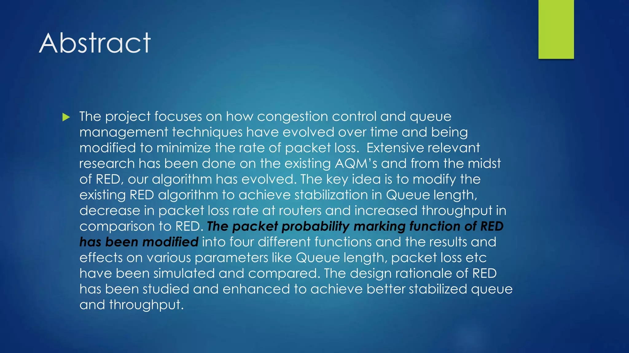


![Results
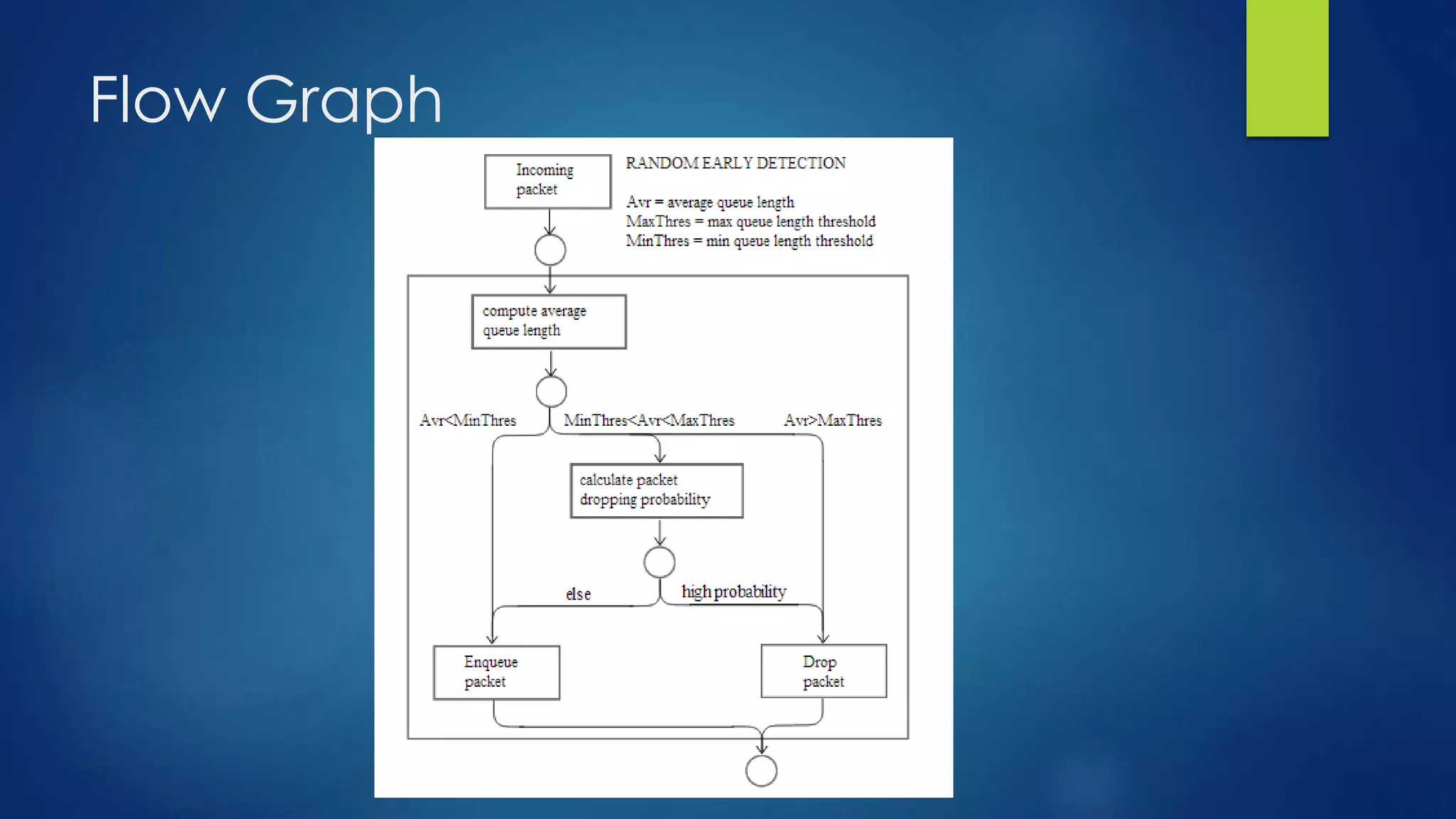
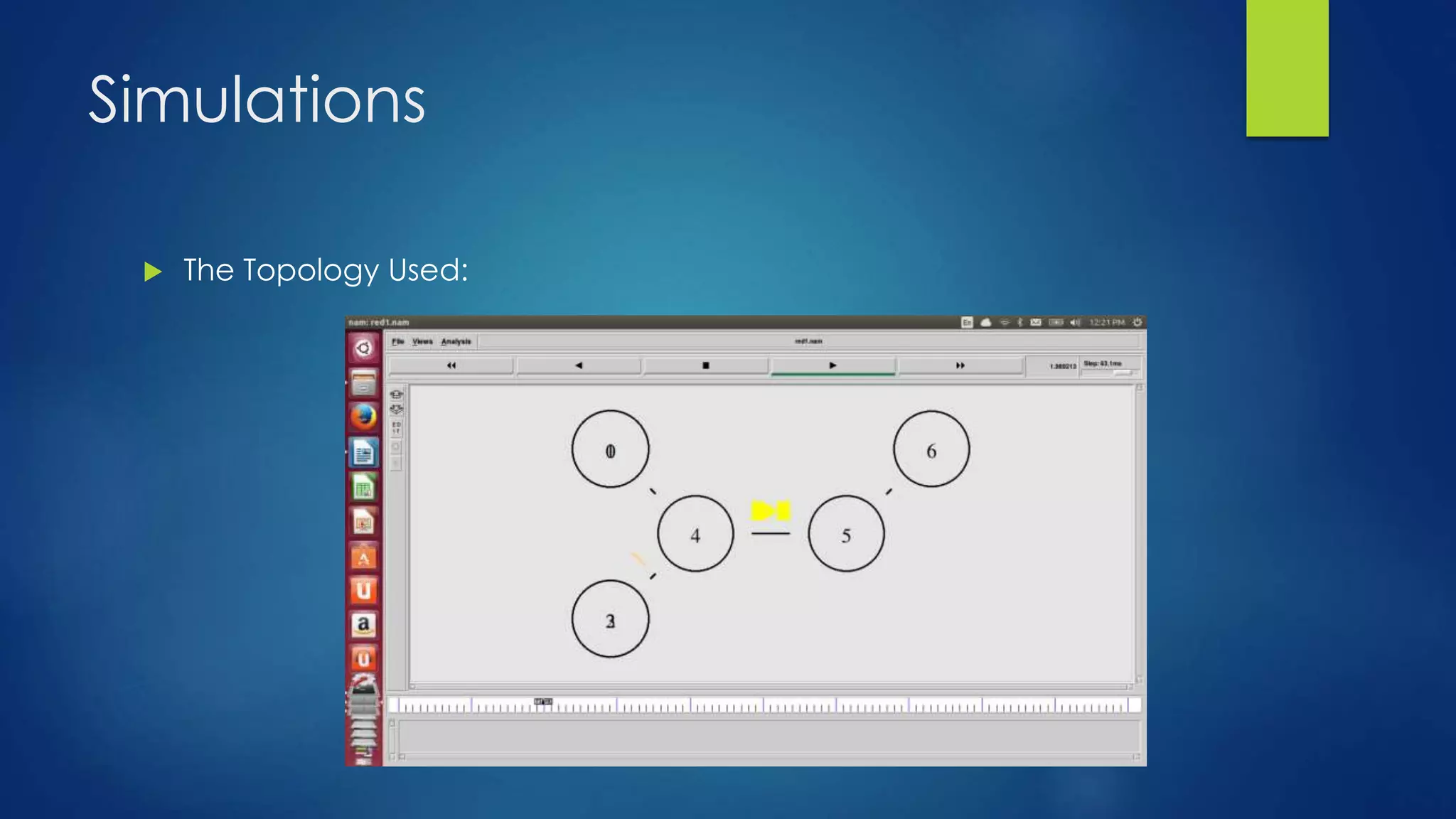
Simulation Topology
(scenario [15,45])
Modified RED
Drop Tail](https://image.slidesharecdn.com/modifiedred-140529105545-phpapp01/75/Analysis-and-Evolution-of-AQM-Algortihms-23-2048.jpg)
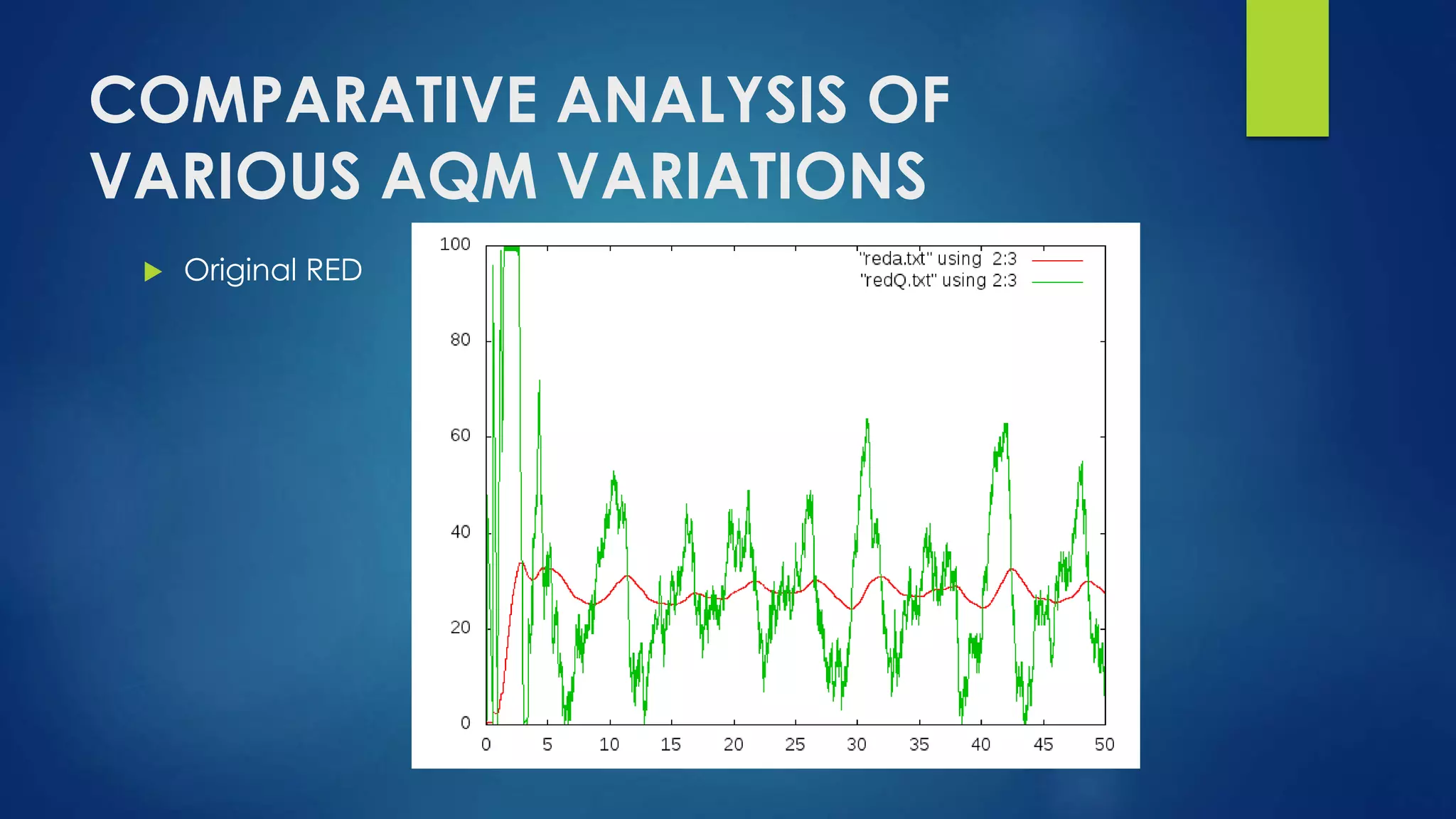
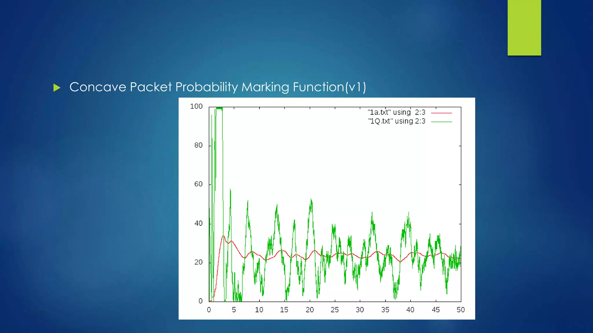
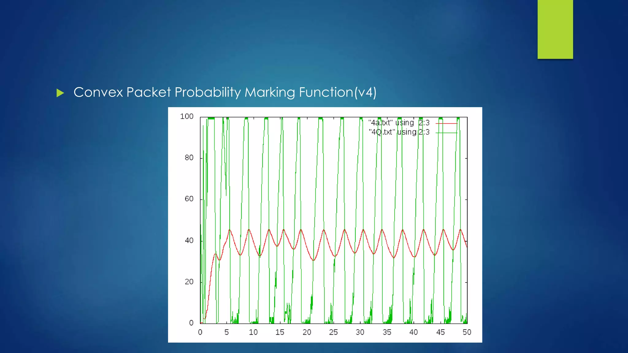
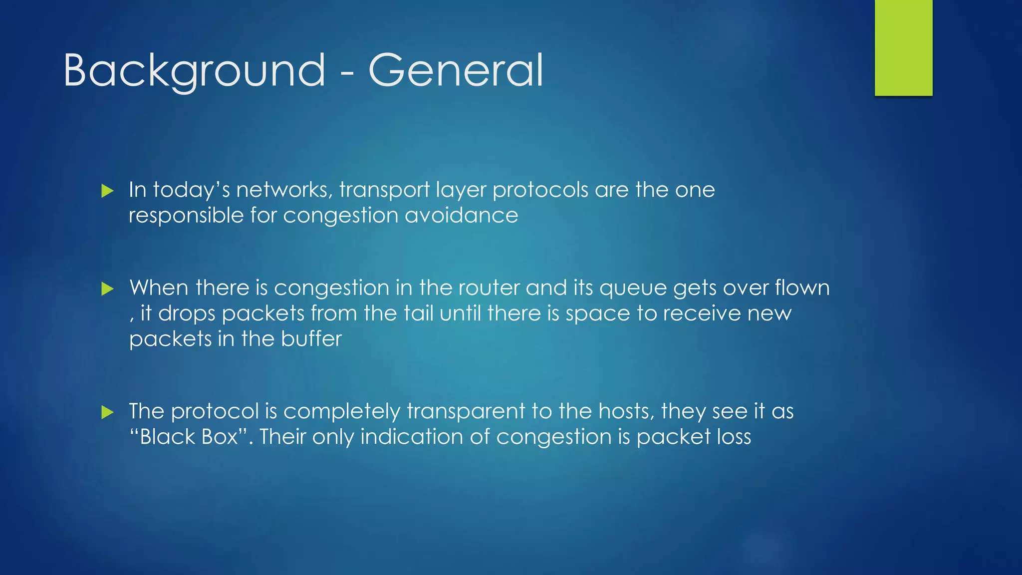
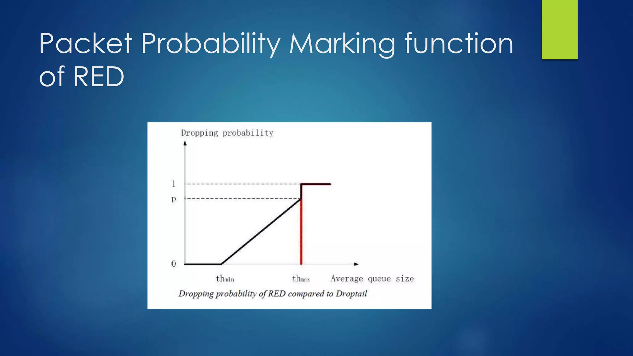
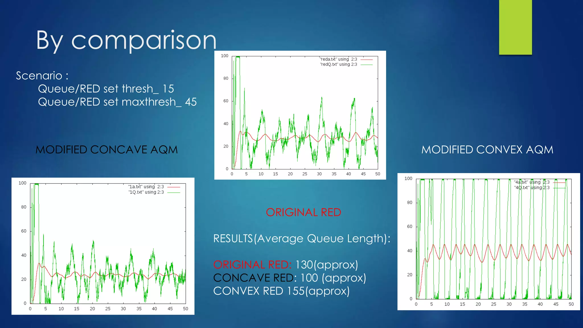
![FINDINGS & CONCLUSION
Queue Size
From the plot, we can see that v1 keeps the
average queue size at a lower level than regular
RED, while v4 keeps the average queue size at a
higher level than regular RED. This is expected as
v1 is always above the original linear function
given the same average queue size value in the
range of [th_min, th_max], in other words, v1 is
more aggressive in terms of dropping packets
when the average queue size is between th_min
and th_max. On the contrast, v4 is less aggressive
than regular RED.](https://image.slidesharecdn.com/modifiedred-140529105545-phpapp01/75/Analysis-and-Evolution-of-AQM-Algortihms-29-2048.jpg)
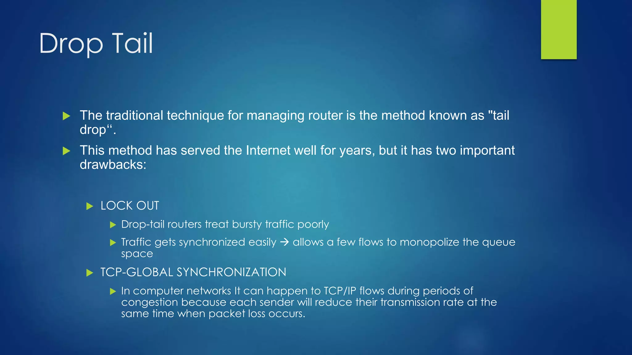
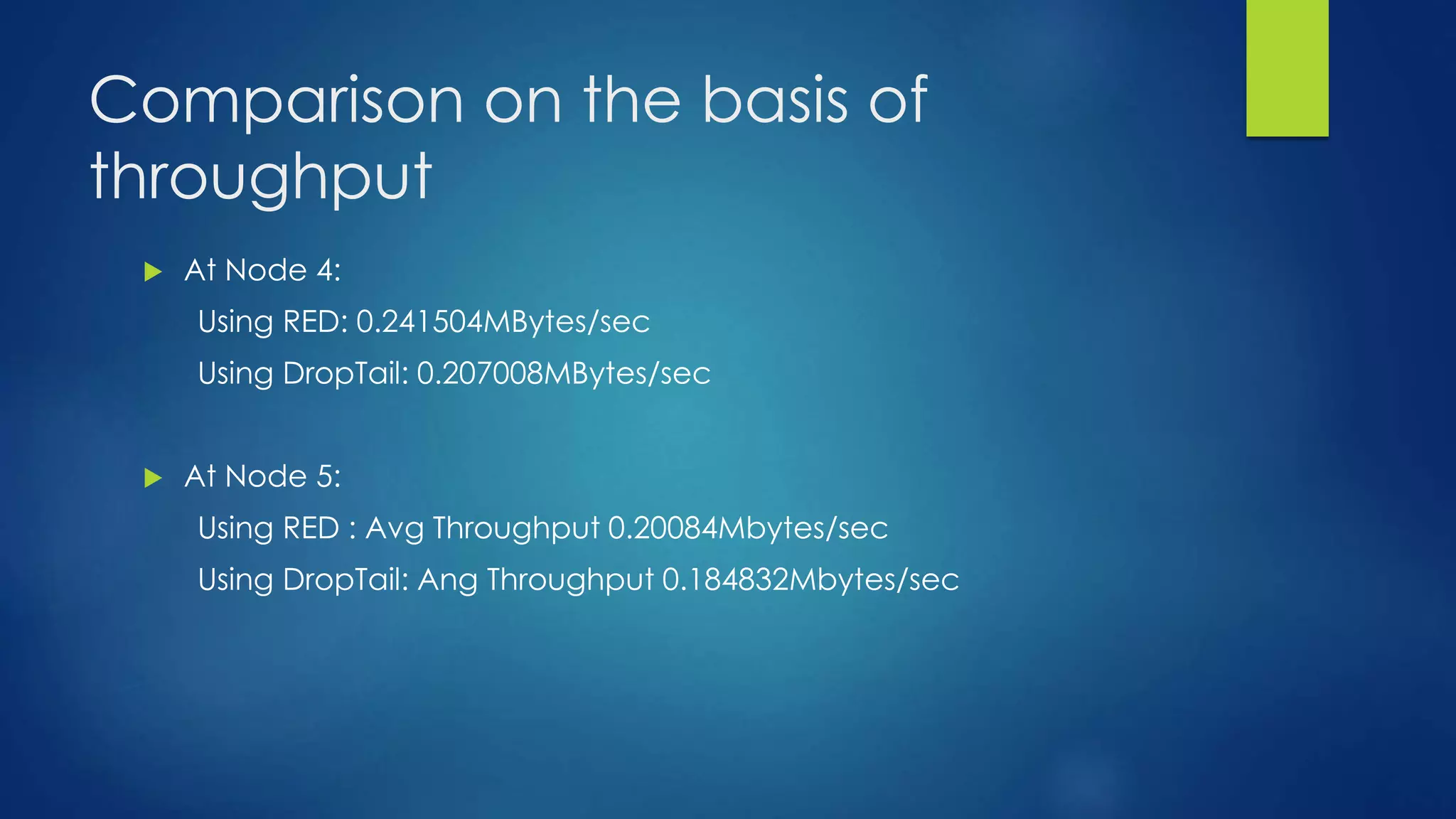
![Scenario[minp,maxp] Function/AQM Packet Sent Packet Lost % Packet Loss
[15,45] RED 18736 27 1.44
[15,45] Concave function (v1) 18717 23 1.22
[15,45] Piece wise Linear(v2) 18698 28 1.49
[15,45] Piece wise Linear(v3) 18459 27 1.46
[15,45] Convex function (v4) 18194 44 2.41
[20,60] RED 18671 25 1.33
[20,60] Concave function (v1) 18712 28 1.49
[20,60] Piece wise Linear(v2) 18636 26 1.39
[20,60] Piece wise Linear(v3) 18373 33 1.79
[20,60] Convex function (v4) 18025 33 1.83
[25,75] RED 18645 29 1.55
[25,75] Concave function (v1) 18657 26 1.39
[25,75] Piece wise Linear(v2) 18648 24 1.28
[25,75] Piece wise Linear(v3) 18579 25 1.34
[25,75] Convex function (v4) 17773 20 1.12
[30,90] RED 18511 26 1.40
[30,90] Concave function (v1) 18564 25 1.34
[30,90] Piece wise Linear(v2) 18564 27 1.45
[30,90] Piece wise Linear(v3) 18522 22 1.18
[30,90] Convex function (v4) 17773 20 1.125
Table Showing Packet Loss For differect Scenarios & Functions](https://image.slidesharecdn.com/modifiedred-140529105545-phpapp01/75/Analysis-and-Evolution-of-AQM-Algortihms-31-2048.jpg)

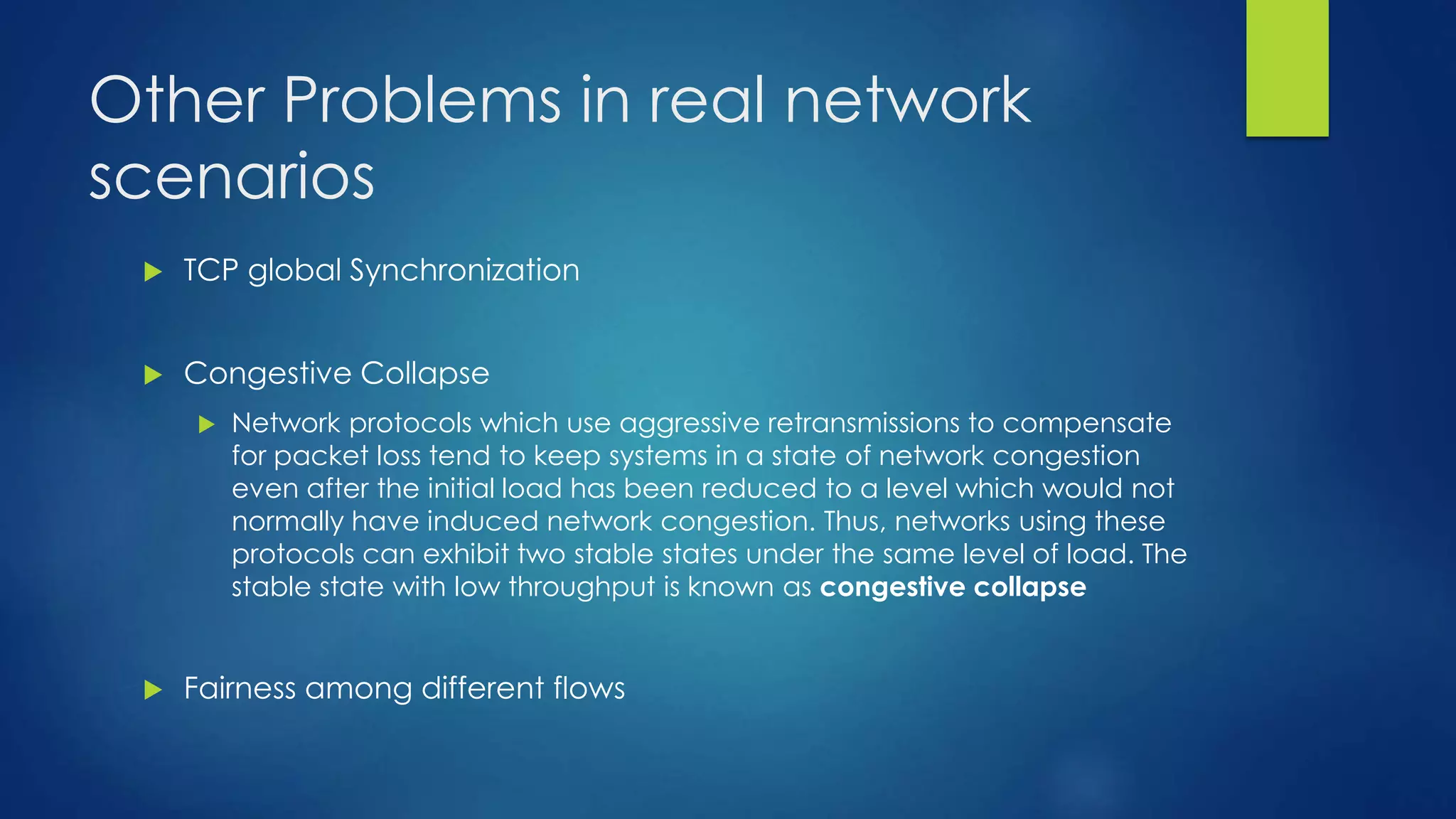
![ISSUES
Installing Ns2.34 in Ubuntu 13.04 (resolved)
Appropriate parameters for running RED. Keeping the number of
nodes high to observe the changes. Leading to overhead.
Appropriate parameters for running RED. Keeping the number of
nodes high to observe changes in throughput.
It was observed that results in a particular scenario [20,60] beg to
differ slightly from other scenarios.](https://image.slidesharecdn.com/modifiedred-140529105545-phpapp01/75/Analysis-and-Evolution-of-AQM-Algortihms-35-2048.jpg)


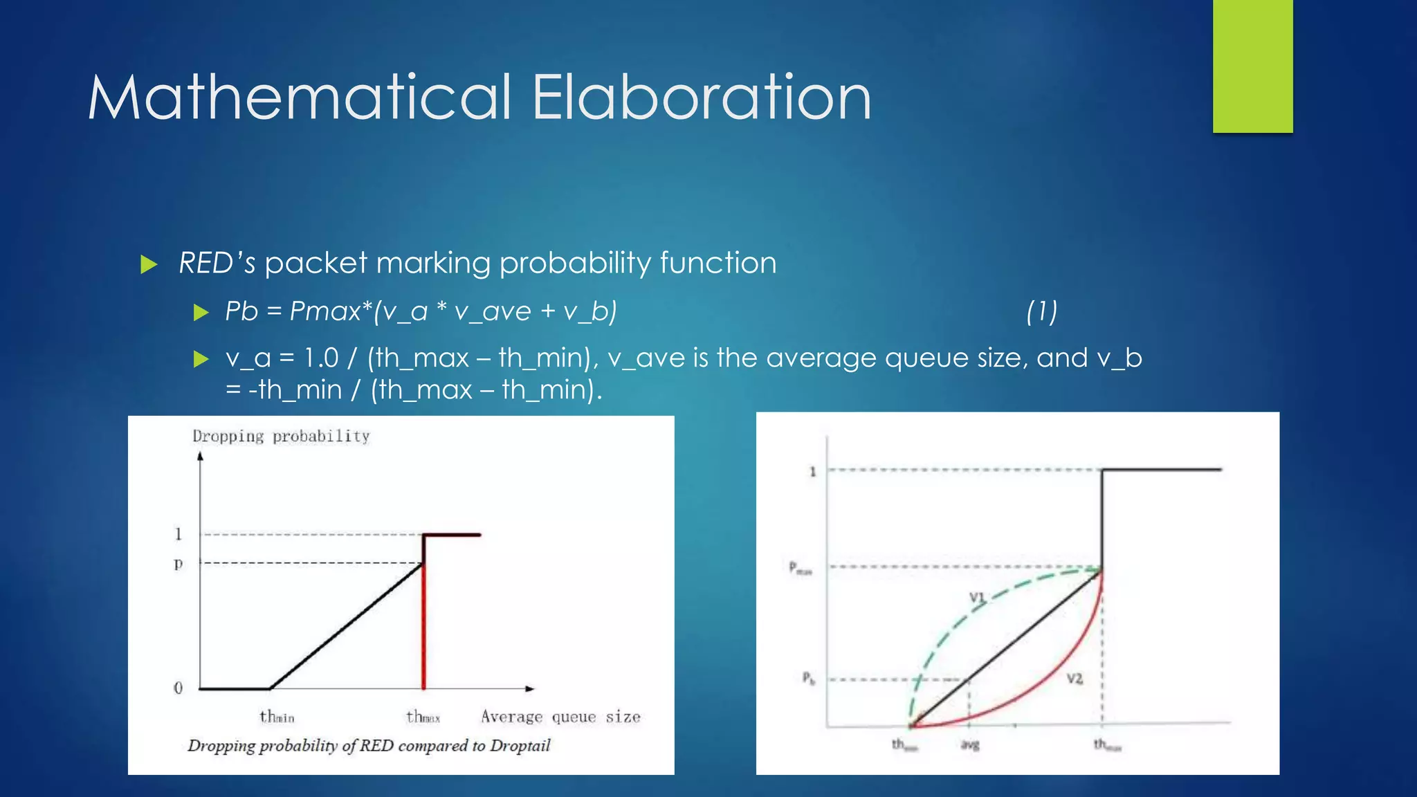


The document details a project by Siddharth Nawani, focusing on the evolution and modification of active queue management (AQM) algorithms, specifically the RED (Random Early Detection) algorithm, to reduce packet loss and improve network throughput. The project includes background analysis of conventional AQM methods, modifications to the RED algorithm, extensive simulation results, and plans for future work to integrate multiple congestion control strategies. Findings indicate that the modified RED variants can maintain lower average queue sizes and reduce packet loss in comparison to standard implementations.