Download to read offline
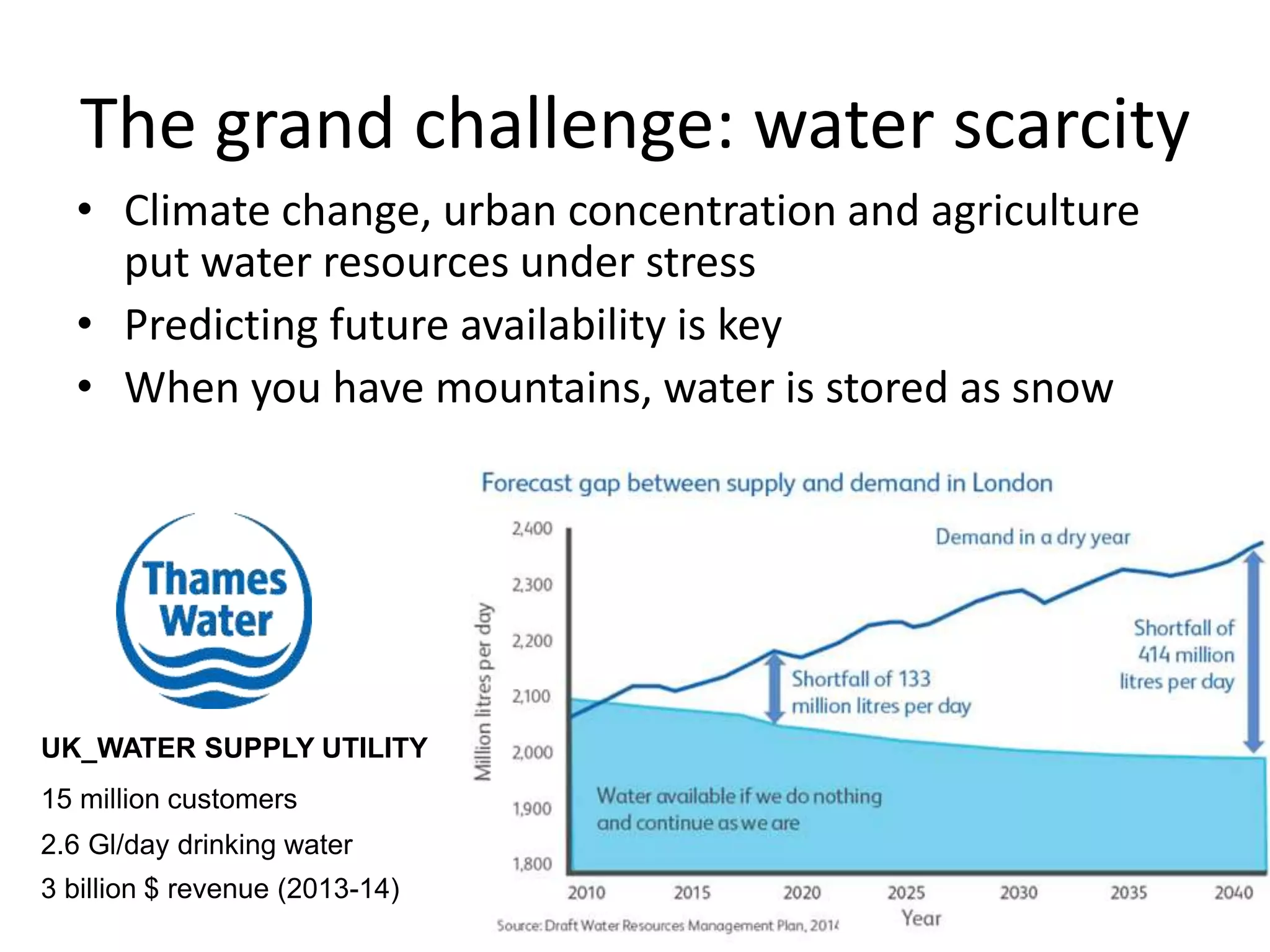
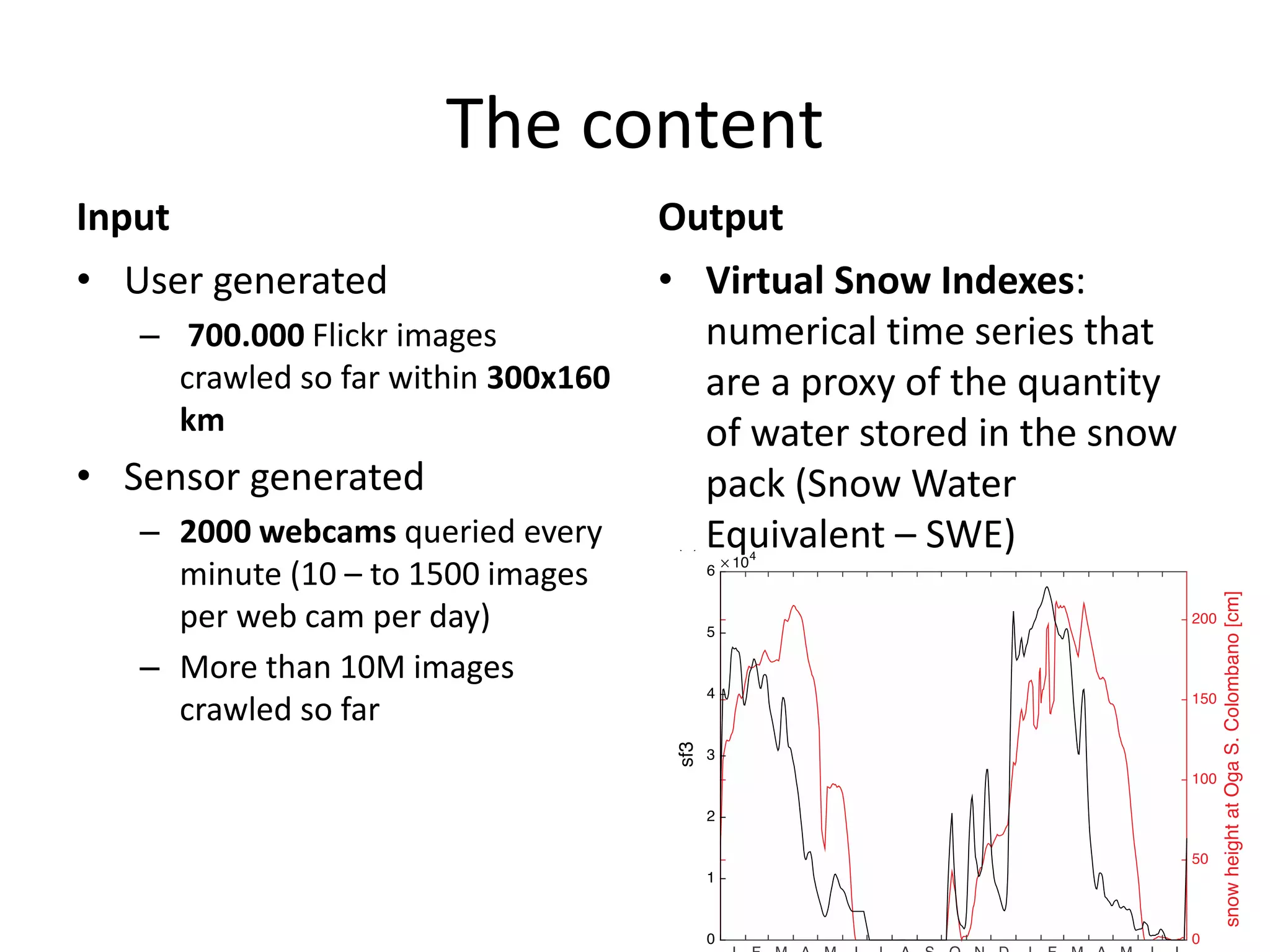
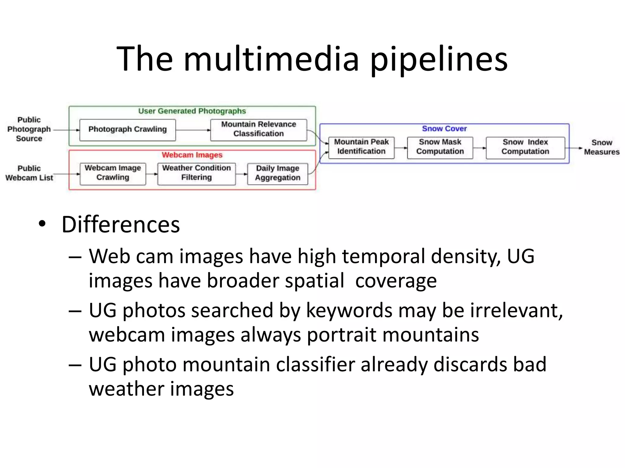
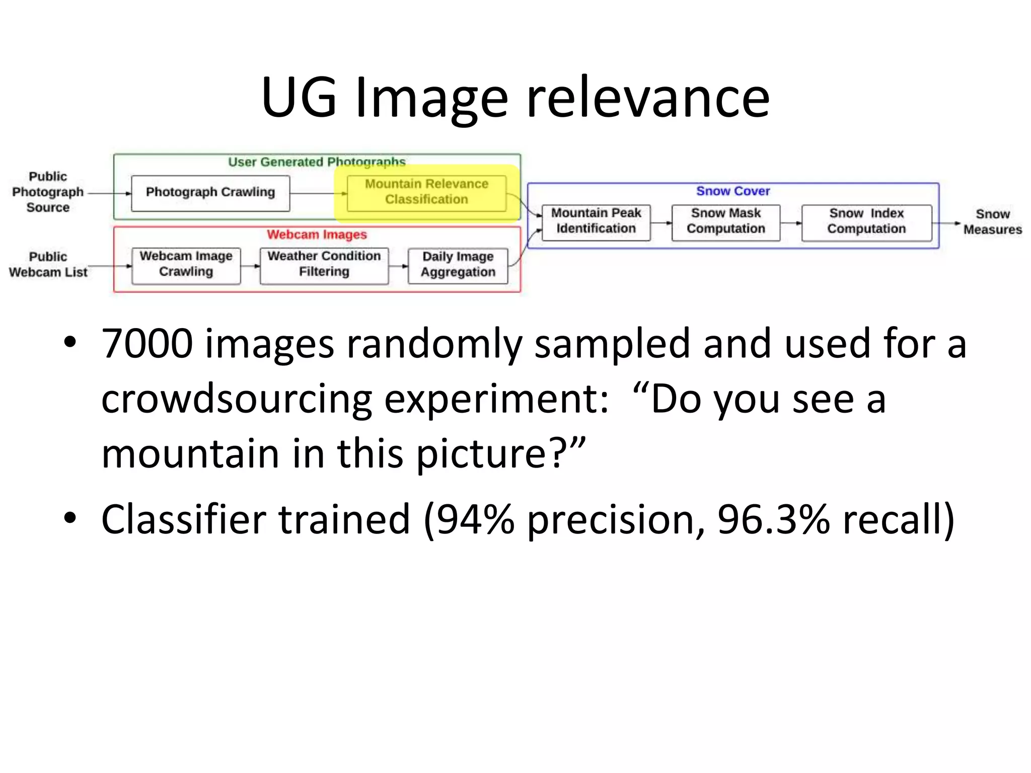
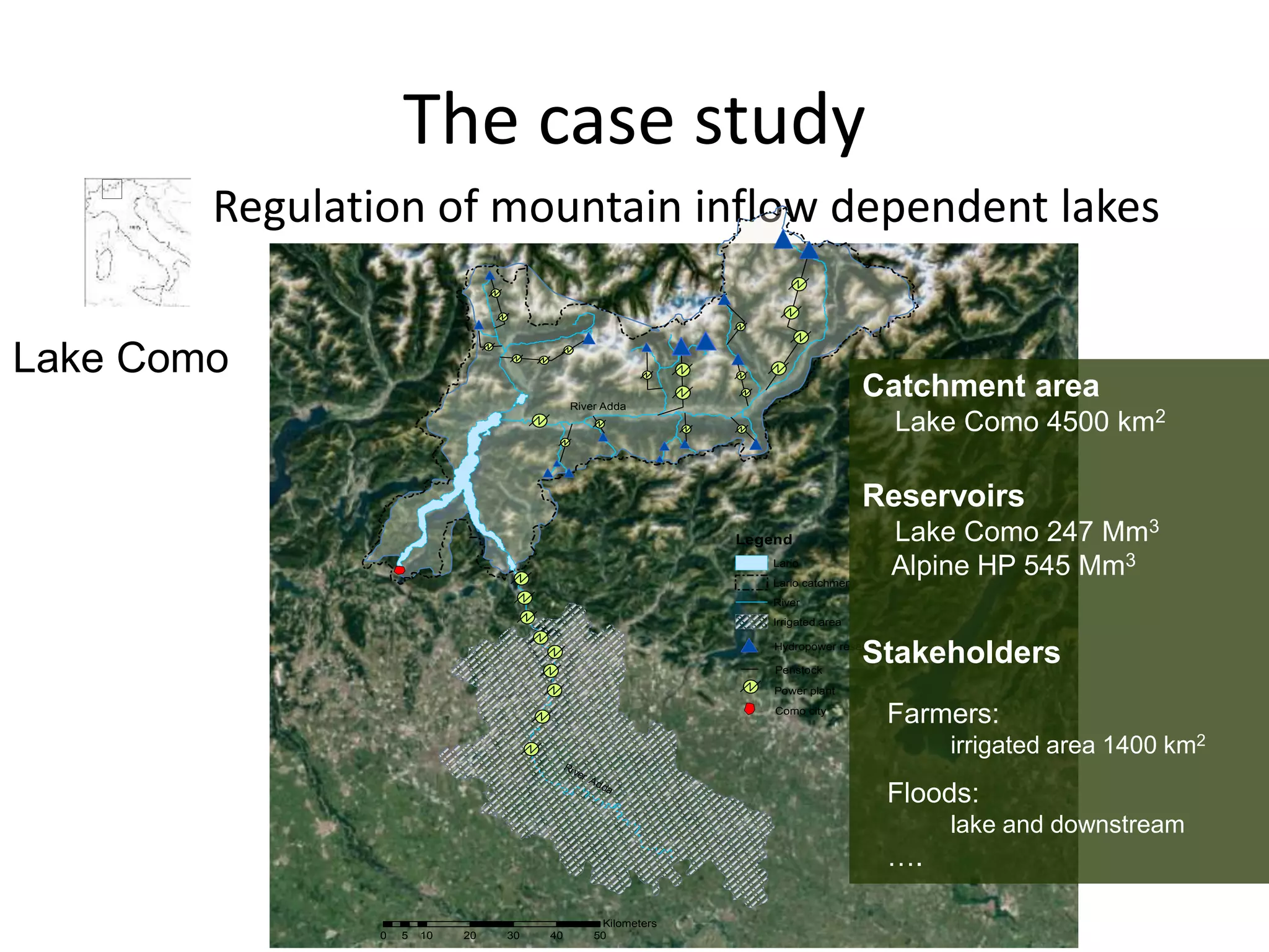


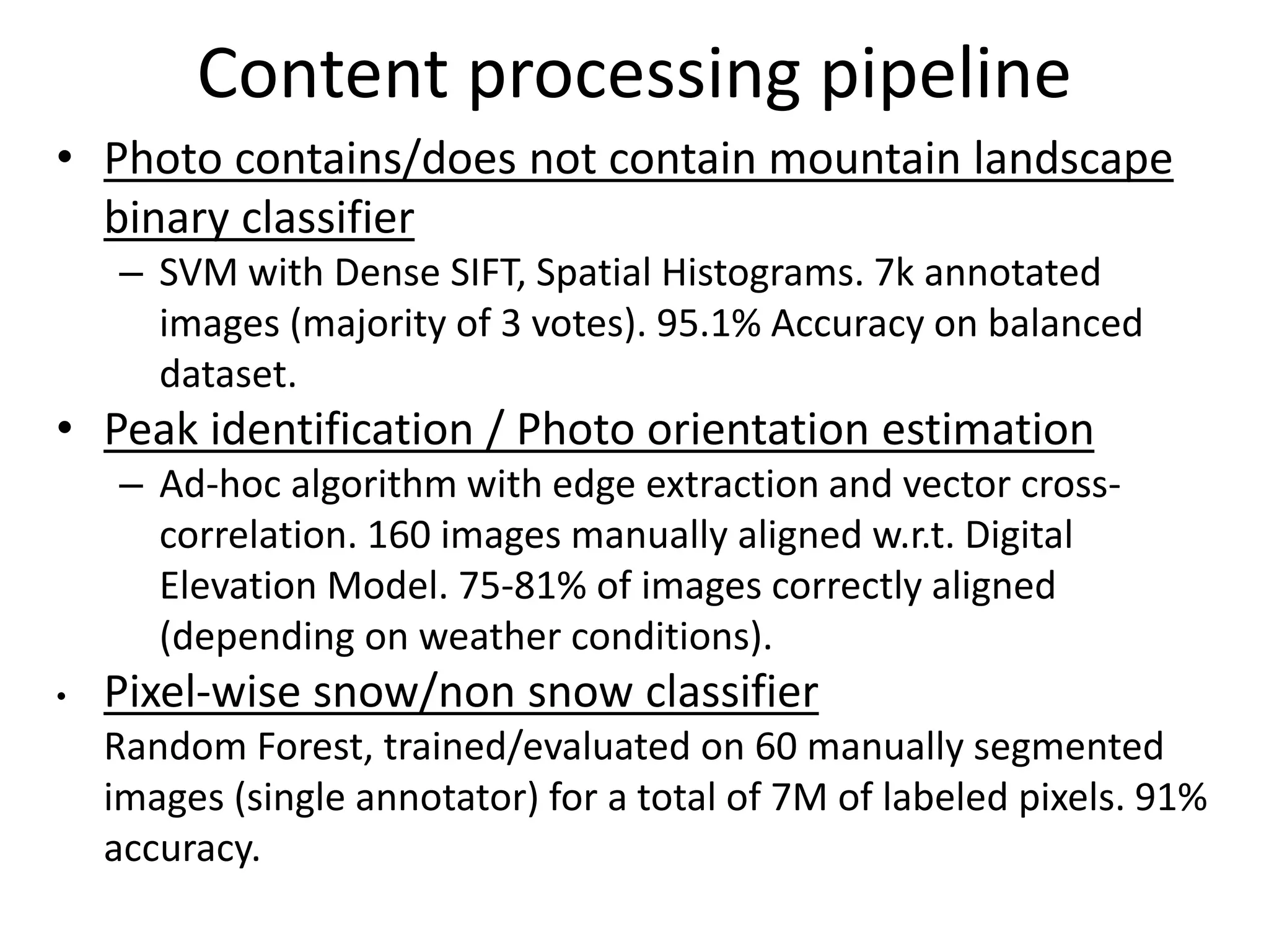


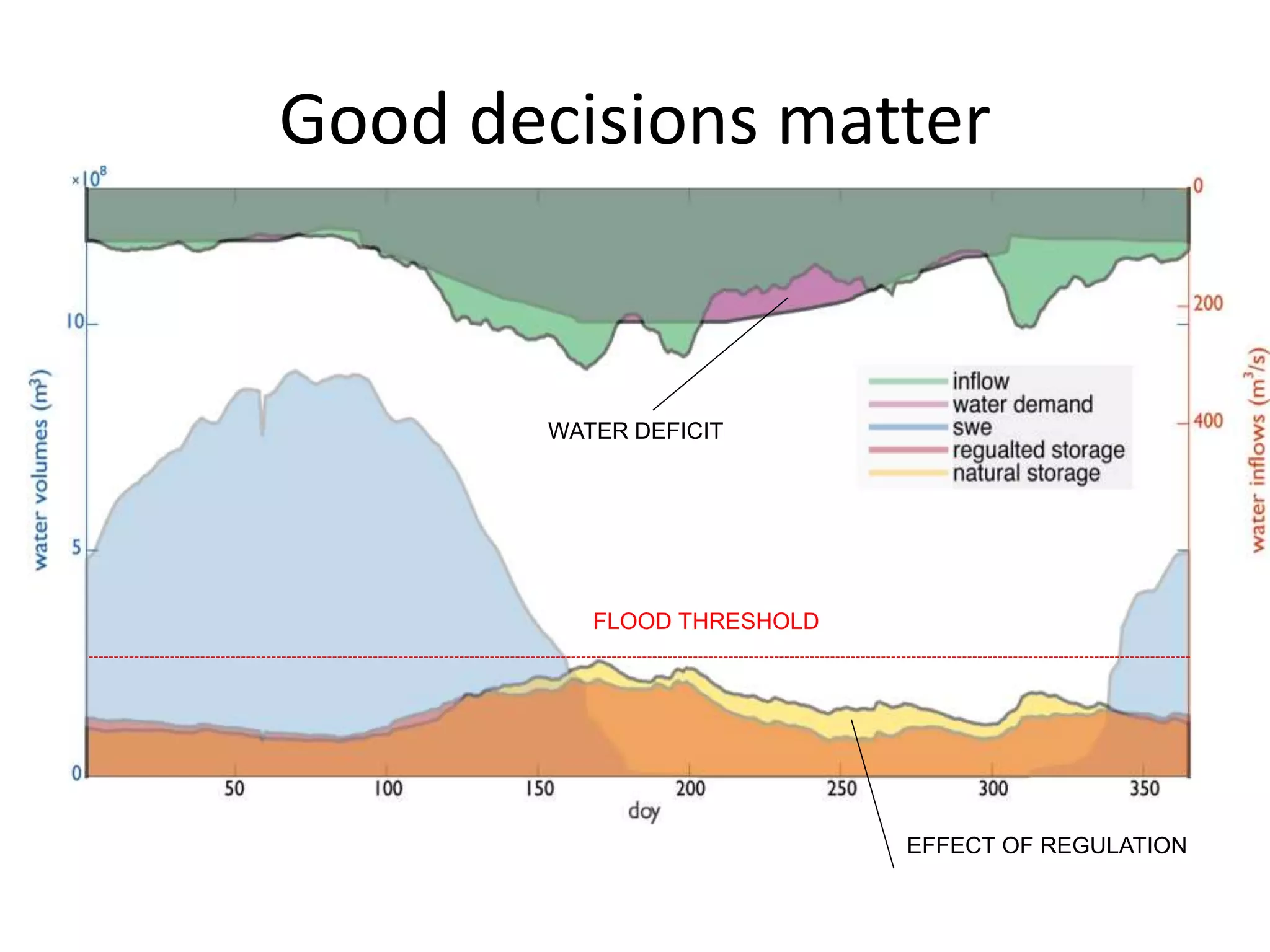
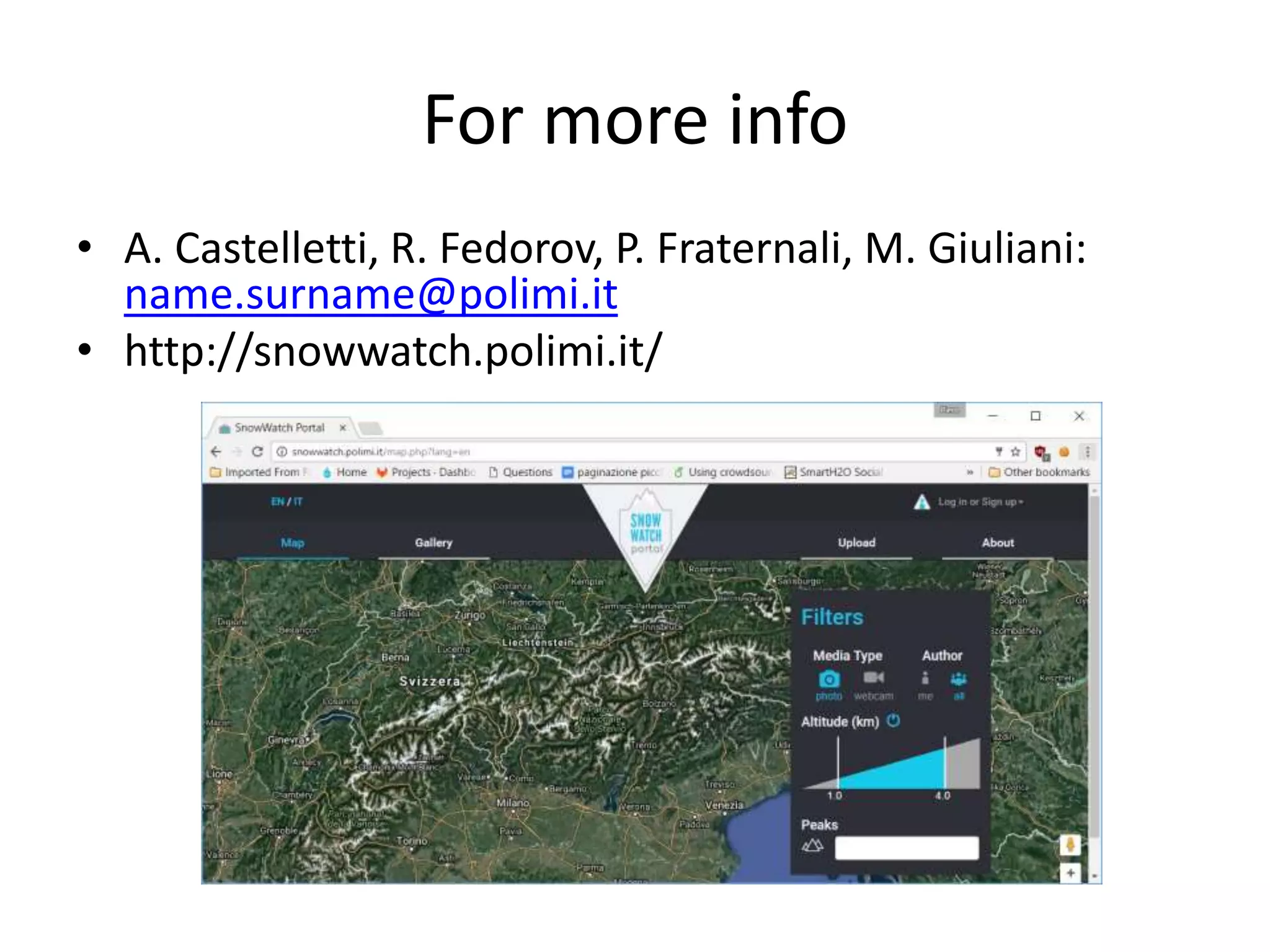

The document discusses the use of public multimedia content, particularly snow images, to enhance water resource management, addressing challenges like water scarcity exacerbated by climate change. It outlines the development of virtual snow indexes from user-generated and sensor-generated data to predict water availability, exploring various methodologies for image classification and policy optimization for lake inflow regulation. The case study focuses on Lake Como, illustrating how the integration of visual data can improve water management decisions while ensuring ecological preservation.


![[IJET-V1I3P9] Authors :Velu.S, Baskar.K, Kumaresan.A, Suruthi.K](https://cdn.slidesharecdn.com/ss_thumbnails/ijet-v1i3p9-150603165341-lva1-app6892-thumbnail.jpg?width=640&height=640&fit=bounds)