This document discusses high-performance computing and numerical algorithms for large-scale scientific simulations. It describes how modern HPC architectures have increasing numbers of cores but declining memory per core, posing challenges for numerical algorithms. High-order numerical methods that efficiently use computing power while maintaining solution accuracy are needed. The document also provides an overview of the FLASH astrophysics simulation code, its capabilities, and examples of simulations performed.

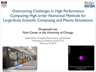
1. Dongwook Lee
Flash Center at the University of Chicago
Overcoming Challenges in High Performance
Computing: High-order Numerical Methods for
Large-Scale Scientific Computing and Plasma Simulations
Department of Applied Mathematics and Statistics
University of California, Santa Cruz
February 24, 2014
FLASH Simulation of a 3D Core-collapse Supernova
Courtesy of S. Couch
MIRA, BG/Q, Argonne National Lab
49,152 nodes, 786,432 cores

2. Computer Genius
Introducing…
Math GeniusHigh Performance Computing

3. High Performance Computing (HPC)
‣To solve large problems in science, engineering, or
business
‣Modern HPC architectures have
▪ increasing number of cores
▪ declining memory/core
‣This trend will continue for the foreseeable future

4. High Performance Computing (HPC)
‣This tension between computation & memory brings a
paradigm shift in numerical algorithms for HPC
‣To enable scientific computing on HPC architectures:
▪ efficient parallel computing, (e.g., data parallelism, task
parallelism, MPI, multi-threading, GPU accelerator, etc.)
▪ better numerical algorithms for HPC

5. Numerical Algorithms for HPC
‣Numerical algorithms should conform to the
abundance of computing power and the scarcity of
memory
‣But…
▪ without losing solution accuracy
▪ maintaining maximum solution stability
▪ faster convergence to “correct” solution

6. Large Scale Astrophysics Codes
▪FLASH (Flash group, U of Chicago)
▪ PLUTO (Mignone, U of Torino),
▪ CHOMBO (Colella, LBL)
▪ CASTRO (Almgren,Woosley, LBL, UCSC)
▪ MAESTRO (Zingale, Almgren, SUNY, LBL)
▪ ENZO (Bryan, Norman, Abel, Enzo group)
▪ BATS-R-US (CSEM, U of Michigan)
▪ RAMSES (Teyssier, CEA)
▪ CHARM (Miniati, ETH)
▪ AMRVAC (Toth, Keppens, CPA, K.U.Leuven)
▪ ATHENA (Stone, Princeton)
▪ ORION (Klein, McKee, U of Berkeley)
▪ ASTROBear (Frank, U of Rochester)
▪ ART (Kravtsov, Klypin, U of Chicago)
▪ NIRVANA (Ziegler, Leibniz-Institut für Astrophysik Potsdam), and others
Peta- Scale
Current HPC
Future HPC
Giga- Scale
Current Laptop/Desktop
?

7. The FLASH Code
‣FLASH is is free, open source code for astrophysics and HEDP
!
▪ modular, multi-physics, adaptive mesh refinement (AMR), parallel
(MPI & OpenMP), finite-volume Eulerian compressible code for
solving hydrodynamics and MHD
!
▪ professionally software engineered and maintained (daily
regression test suite, code verification/validation), inline/online
documentation
!
▪ 8500 downloads, 1500 authors, 1000 papers
!
▪ FLASH can run on various platforms from laptops to
supercomputing (peta-scale) systems such as IBM BG/P and BG/Q

8. FLASH Simulations
cosmological
cluster formation supersonic MHD
turbulence
Type Ia SN
RT
CCSN
ram pressure stripping
laser slab
rigid body
structure
Accretion Torus
LULI/Vulcan experiments: B-field
generation/amplification

9. High Energy Density Physics
!
▪ multi-temperature (1T, 2T, & 3T) in
hydrodynamics and MHD
▪ implicit electron thermal conduction
using HYPRE
▪ flux-limited multi-group approximation
for diffusion radiative transfer
▪ multi-material support: EoS and
opacity (tabular & analytic)
▪ laser energy deposition using ray
tracing
▪ rigid body structures
FLASH’s Multi-Physics Capabilities
Astrophysics
!
▪ hydrodynamics, MHD, RHD,
cosmology, hybrid PIC
▪ EoS:
gamma laws, multi-gamma,
Helmholtz
▪ nuclear physics and other source
terms
▪ external gravity, self-gravity
▪ active and passive particles
(used for PIC, laser ray tracing,
dark matter, tracer particles)
▪ material properties
✓Fortran, C, Python > 1.2 million lines (25% comments!)
✓Extensive documentations available in User’s Guide
✓Scalable to tens of thousand processors with AMR

10. Numerical Algorithm
Astrophysics
High Energy Density Physics
My Research Work
coming soon!

11. My Collaborators
▪ M. Ruszkowski (U of Michigan)
▪ J. ZuHone (NASA, Goddard)
▪ K. Murawski (UMSC, Poland)
▪ F. Cattaneo (U of Chicago)
▪ P. Ricker (UIUC)
▪ M. Bruggen, R. Banerjee (U of Hamburg)
▪ M. Shin (U of Oxford)
▪ P. Oh, S. Ji (UCSB)
▪ I. Parrish (UCB)
▪ E. Zweibel (UWM)
▪ A. Deane (UMD)
▪ A. Dubey, P. Colella, J. Bachan, C. Daley (LBL)
▪ C. Federrath (Monash U,Australia)
▪ R. Fisher (UM Darthmouth)
▪ G. Gianluca, J. Meinecke (U of Oxford)
▪ P. Drake (U of Michigan)
▪ R.Yurchak (LULI, France)
▪ F. Miniati (ETH, Switzerland)
Astrophysics
High Energy
Density Physics

12. Parallelization, Optimization & Speedup
‣Adaptive Mesh Refinement with Paramesh
▪standard MPI (Message Passing Interface)
parallelism
▪domain decomposition distributed over
multiple processor units
▪distributed memory
uniform grid octree-based
block AMR
patch-based AMR
Single block

13. Parallelization, Optimization & Speedup
16 cores/node
16 GB/node
4 threads/core

14. ▪ 5 leaf blocks in a single MPI rank
▪ 2 threads/core (or 2 threads/rank)
Parallelization, Optimization & Speedup
thread block list thread within block
‣Multi-threading (shared memory) using OpenMP directives
▪more parallel computing on BG/Q using hardware threads on a core
▪ 16 cores/node, 4 threads/core

15. FLASH Scaling Test on BG/Q
VESTA:
2 racks
1024 nodes/rack
MIRA:
48 racks
1024 nodes/rack
BG/Q:
16 cores/node
4 threads/core
16GB/core
512
(4k)
1024
(8k)
2048
(16k)
4096
(32k)
8192
(64k)
16384
(128k)
32768
(256k)
Mira nodes (ranks), 8 threads/rank
0
2
4
6
8
10
108
corehours/zone/step
0
5
10
15
20
25
107
corehours/zone/IOwrite
Total evolution
MHD
Gravity
Grid
IO (1 write)
⌫-Leakage
Ideal
RTFlame, strong scaling: 4 threads/rank CCSN, weak scaling: 8 threads/rank

16. Numerical Algorithms,
Solvers,
Godunov Schemes,
High-Order Methods,
Oscillations,
Stability,
Convergence,
etc…

17. Discretization Approaches
‣FiniteVolume (FV)
▪shock capturing, compressible flows, structured/unstructured grids
▪hard to achieve high-order (higher than 2nd order)
‣Finite Difference (FD)
▪smooth flows, incompressible, high-order methods
▪non-conservative, simple geometry
‣Finite Element (FE)
▪arbitrary geometry, basis functions, continuous solutions
▪hard coding, problems at strong gradients
‣Spectral Element (SE)
‣Discontinuous Galerkin (DG)

18. FV Godunov Scheme for Hyperbolic System
‣The system of conservation laws
(hyperbolic PDE) in 1D:
!
!
!
!
‣A discrete integral form (i.e., finite-
volume):
!
!
!
‣Godunov scheme seeks for time averaged
fluxes at each interface by solving the self-
similar solution of the Riemann problem:
!
!
@U
@t
+
@F
@x
= 0
Un+1
i = Un
i
t
x
(Fn
i+1/2 Fn
i 1/2)
U⇤
i+1/2(x/t) = RP(Un
i , Un
i+1),
Fn
i+1/2 = F(U⇤
i+1/2(0))
= F(Un
i , Un
i+1)
t
x
U⇤
(x/t)
Un
i+1Un
i
Riemann Fan
rarefaction
contact
discontinuity
shock
piecewise-constant (first-order)

19. A Discrete World of FV
U(x, tn
)
xixi 1 xi+1

20. A Discrete World of FV
u(xi, tn
) = Pi(x), x 2 (xi 1/2, xi 1/2)
xixi 1 xi+1
piecewise polynomial reconstruction
on each cell
uL = Pi+1(xi+1/2)uR = Pi(xi+1/2)

21. A Discrete World of FV
xixi 1 xi+1
At each interface we solve a RP and obtain Fi+1/2

22. A Discrete World of FV
We are ready to advance our solution in time and
get new volume-averaged states
Un+1
i = Un
i
t
x
(Fi+1/2 Fi 1/2)

23. It Gets Much More Complicated in Reality
▪In 3D we have 6 interfaces per cell
▪2 transverse RPs per each interface
▪12 RPs are needed to for maximum
Courant stability limit, Ca~1
▪Expensive!
x
y
z

24. Computational Advantages In Unsplit Solvers
‣New Efficient Unsplit Algorithm (Lee & Deane, 2009; Lee, 2013)
‣Most unsplit schemes need 12 Riemann solves (see Table)
‣3D Unsplit solvers in FLASH need
▪ 3 Riemann solves in hydro & 6 Riemann solves in MHD with
maximum Courant stability limit, Ca ~ 1
Mignone et al. 2007

25. Stability, Consistency and Convergence
‣Lax Equivalence Theorem (for linear problem, P. Lax, 1956)
▪The only convergent schemes are those that are both consistent and stable
▪Hard to show that the numerical solution converges to the original
solution of PDE; relatively easy to show consistency and stability of
numerical schemes
‣In practice, non-linear problems adopts the linear theory as guidance
▪code verification (code-to-code comparison)
▪code validation (code-to-experiment, code-to-analytical solution
comparisons)
▪self-convergence test over grid resolutions (a good measurement for
numerical accuracy)

26. PLM PPM
High-Order Polynomial Reconstruction
• Godunov’s order-barrier theorem (1959)
• Monotonicity-preserving advection schemes are at most first-order! (Oh no…)
• Only true for linear PDE theory (YES!)
!
• High-order “polynomial” schemes became available using non-linear slope limiters
(70’s and 80’s: Boris, van Leer, Zalesak, Colella, Harten, Shu, Engquist, etc)
• Can’t avoid oscillations completely (non-TVD)
• Instability grows (numerical INSTABILITY!)
FOG

27. Shu-Osher Problem:1D Mach 3 Shock

28. Low-Order vs. High-Order
1st Order
High-Order
Ref. Soln
1st order: 3200 cells (50 MB), 160 sec, 3828 steps
vs
High-order: 200 cells (10 MB), 9 sec, 266 steps

29. Circularly Polarized Alfven Wave (CPAW)
▪A CPAW problem propagates
smoothly varying oscillations of
the transverse components of
velocity and magnetic field
▪The initial condition is the exact
nonlinear solutions of the MHD
equations
▪The decay of the max ofVz and
Bz is solely due to numerical
dissipation: direct measurement
of numerical diffusion (Ryu, Jones
& Frank,ApJ, 1995)
Fig. A.3. Long term decay of circularly polarized Alfvén waves after 16.5 time units, corresponding to $ 100 wave periods. In the left panel, we plot the
A. Mignone et al. / Journal of Computational Physics 229 (2010) 5896–5920 5907

30. Outperformance of High-Order: CPAW
L1 norm error
avg. comp.
time / step
32 256
0.221 (x5/3)sec 38.4 sec
Source: Mignone & Tzeferacos, 2010, JCP
▪PPM-CT (overall 2nd
order): 2h42m50s
▪MP5 (5th order):
15s(x5/3)=25s
!
▪More computational
work & less memory
▪Better suited for HPC
▪Easier in FD; harder in FV
▪High-orders schemes are
better in preserving
solution accuracy on AMR

31. Numerical Oscillations
‣ In general, numerical (spurious) oscillations happen
‣near steep gradients (Gibbs’ oscillation)
‣lack of numerical dissipation (high-order schemes)
‣lack of numerical stability (Courant condition)
‣if present, numerical solution is invalid
‣Controlling oscillations is crucial for solution accuracy & stability
‣More complicated situations (see LeVeque):
‣carbuncle/even-odd decoupling instability (Quirk, 1992)
‣start-up error
‣slow-moving shocks (see next)

32. Numerical Oscillations
‣Slow-moving shocks:
‣unphysical oscillations can exponentially grow in time, especially near
strong and slowly moving shocks (Woodward & Colella, 1984)
‣Jin &Liu (1996); Donat & Marquina (1996); Karni & Canic (1997);Arora
& Roe (1997); Striba & Donat (2003); Lee (2010)
First-order Godunov method (Source: LeVeque)

33. PPM Oscillations for Slow-Moving Shocks
✓Standard 3rd order PPM suffers from
unphysical oscillations for MHD Brio-
Wu Shock Tube (Brio-Wu, 1988)
✓Fix is available by applying an upwind
slope limiter for PPM (Lee, 2010)
✓Upwind PPM behaves very similar to
WENO5, reducing oscillations!
standard PPM
(Colella & Woodward, 1984)
upwind PPM (Lee, 2010)
WENO5 (Jiang & Shu, 1996)
Bad!
Improved!
Reference solution

34. Traditional High-Order Schemes
‣Traditional approaches to get (N+1)th high-order schemes take Nth
degree polynomial
▪only for normal direction (e.g., FOG, MH, PPM, ENO,WENO, etc)
▪with monotonicity controls (e.g., slope limiters, artificial viscosity)
‣ High-order in FV is tricky (when compared to FD)
▪volume-averaged quantities (quadrature rules)
▪preserving conservation w/o losing accuracy
▪higher the order, larger the stencil
▪high-order temporal update (ODE solvers, e.g., RK3, RK4, etc.)
2D stencil for
2nd order PLM
2D stencil for
3rd order PPM

35. High-Order using Gaussian Processes (GP)
▪ Gaussian Processes (GP) are a class of a stochastic processes that yield
sampling data from a function that is probabilistically constrained,
but not exactly known
▪C. Graziani, P. Tzeferacos & D. Lee (Flash, U of Chicago)
▪Our high-order GP interpolation scheme is based on:
▪ samples (i.e., volume-averaged data points) of the function
▪ train the GP model on the samples by means of Bayes’ theorem
▪ the posterior mean function is our high-order interpolant of the
unknown function
▪The result is to pass from an “agnostic” prior model
(a mean function and a covariance kernel) to a data-informed
posterior model (an updated mean function and covariance)

36. Agnostic Prior Model
GP is defined through
(1) a mean function, and
(2) a symmetric positive-definite integral kernel K(x,y):
‣ Mean function
!
!
‣ Kernel (covariance function)
!
!
‣Write
!
!
‣The likelyhood function (the probability of f given the GP model)

37. ‣Want to predict an unknown function f probabilistically at a new
point x*
!
!
‣ Then the augmented likelyhood function is
!
!
!
where
Data-Informed Posterior Model
The result is to pass from an agnostic prior model (a mean
function and a covariance kernel) to a data-informed posterior
model (an updated mean function and covariance)

38. ‣ Bayes’ Theorem gives
Updated Mean Function
The result is to pass from an agnostic prior model (a mean
function and a covariance kernel) to a data-informed posterior
model (an updated mean function and covariance)
Our high-order
interpolated value:
a Gaussian probability
distribution on the
unknown function
value f*

39. Truly Multidimensional Use of Stencil
The current GP interpolation method in FLASH for smooth
flow tests. For this, we use square exponential (SE) convariance
and interpolate on “blocky sphere” of radius R
C1
‣ SE covariance has the property of having a native functions, thus can
provide with spectral convergence rates when the underlying approximated
function is itself C1
2D stencil for GP
2D stencil for
2nd order PLM 2D stencil for
3rd order PPM

40. Revisited:1D Mach 3 Shock
!
PLM on 1600
GP (spectral)
WENO-Z (5)
PPM (3)
PLM (2)
FOG (1)

41. Results on Smooth Flows 1
• 2D advection of an isentropic vortex along the domain
diagonal on a periodic box ( , )R = 2 = 6

42. Results on Smooth Flows II
• 1D advection of Gaussian profile ( , )= 12R = 2

43. Exponential Convergence Rate
• 1D advection of Gaussian profile ( , )= 12R = 2
spatial error
dominance
temporal error
dominance

44. Implicit Solver in Unsplit Hydro
‣Spatial parallelism & optimization (MPI, multi-threading, numerical
algorithm improvements, coding optimizations)
‣Temporal optimization:
▪overcome small diffusion (parabolic PDE) time scales
▪Jacobian-Free Newton-Krylov fully implicit solver (e.g., Knoll and
Keys, 2004;Toth et al., 2006) for unsplit hydro solver
▪ NSF grant (PHY-0903997), 2009-2012, $400K
▪ Dongwook Lee (PI), Guohua Xia (postdoc), Shravan Gopal &
Prateeti Mohapatra (scientists)
▪ GMRES with preconditioner

45. Future ApplicationsSUBMITTED TO APJ ON 2013 OCTOBER 21
Figure 13. Pseudo-color slices of entropy at fou
‣In Core-collapse SN, sound
speed at the core of the proto-
neutron star reaches up to ~1/3
of speed of light
‣This results in a very small
time step is the observed
regions, where there is no shock
‣Hybrid Time Stepping: Implicit
solutions at the core; explicit
solutions elsewhere will bring
huge computing acceleration for
CCSN
FLASH Simulation of a 3D Core-collapse Supernova
Courtesy of S. Couch
entropy

46. Summary
• Novel mathematical algorithms and ideas in designing a scientific code,
and performing state-of-art simulations are the most important key to
success in scientific computing on HPC
!
• High-order method is a good approach to embody the desired
tradeoff between memory and computation in future HPC
!
• Building a good large-scale scientific code with computational
accuracy, stability, efficiency, modularity, especially with multi-physics
capabilities requires to combine various research fields, including
mathematics, physics (and other fields of sciences) and computer
science

47. Future Work!
!
▪More high-order reconstruction methods
▪High-order quadrature rules for multi-dimensions
▪More studies on GP
▪ covariance kernels, applications on AMR
prolongations, more convergence studies, GP for
FD, etc.
▪High-order temporal integrations (RK3, RK4, etc.)
▪Hybrid explicit-implicit solvers
!
▪More fine-grained threading
▪Keep up with HPC trends
▪GPU accelerators

48. Type 1a SN (105M hr, 2013)
Shock-Generated Magnetic Fields (40M hr, 2013)
Turbulent Nuclear Combustion (150M hr, 2013)
FLASH’s Recent Computing Time Awards
Core-Collapse SN (30M hr, 2013)

49. Thank you! Questions?
Supersonic Banana Slug

50. Supplementary Slides

51. High-Order Numerical Algorithms
‣ Provide more accurate numerical solutions using
▪ less grid points (=memory save)
▪ higher-order mathematical approximations (promoting
floating point operations, or computation)
▪ faster convergence to solution

52. Unsplit Hydro/MHD Solvers
‣Spatial Evolution (PDE evolution with Finite-volume):
‣Reconstruction Methods:
‣Polynomial-based:1st order Godunov, 2nd order PLM, 3rd order
PPM, 5th order WENO
‣Gaussian Process model-based: spectral-order GP (very new!)
‣Riemann Solvers:
‣Rusanov, HLLE, HLLC, HLLD (MHD), Marquina, Roe, Hybrid
‣Temporal Evolution (ODE evolution):
‣2nd-order characteristic tracing (predictor-corrector type) method