2011 santiago marchi_souza_araki_cobem_2011

Proceedings of COBEM 2011 21
st
Brazilian Congress of Mechanical Engineering
Copyright © 2011 by ABCM October 24-28, 2011, Natal, RN, Brazil
PERFORMANCE OF THE MULTIGRID METHOD WITH ALTERNATIVE
FORMULATIONS FOR THE NAVIER-STOKES EQUATIONS
Cosmo Damião Santiago, cosmo@utfpr.edu.br
Federal Technology University of Paraná (UTFPR) – Campus of Apucarana
Rua Marcílio Dias, 635, CEP 86812-460 - Apucarana, PR, Brazil.
Carlos Henrique Marchi, marchi@ufpr.br
Department of Mechanical Engineering (DEMEC) – Federal University of Paraná (UFPR), Curitiba - PR, Brazil
Leandro Franco de Souza, lefraso@icmc.usp.br
University of São Paulo (USP) - Department of Applied Mathematics and Statistics – Campus of São Carlos
Av. Trabalhador São-Carlense, 400, CEP 13566-590 São Carlos, SP, Brazil
Luciano Kiyoshi Araki, araki@ufpr.br
Department of Mechanical Engineering (DEMEC) – Federal University of Paraná (UFPR), Curitiba - PR, Brazil
Abstract. The performance of the geometric multigrid method in solving the two-dimensional incompressible Navier-
Stokes equations is studied. Two alternative formulations are employed for the classical lid-driven cavity flow
problem: the recent streamfunction-velocity and the streamfunction-vorticity. The main objective of this work is the
CPU time reduction by the finding of optimum values for the following multigrid parameters: inner iterations and the
number of grid levels, for different Reynolds numbers and different grid sizes. The performance of the two formulations
is also compared. The equations are discretized using the Finite Difference Method, with second-order central
differencing approximations and uniform grids. The systems of linear equations are solved with the use of the
Successive Over-Relaxation (SOR) method, associated to the geometric multigrid. The results show that: the
streamfunction-vorticity formulation presents smaller CPU times; the efficiency of the multigrid decreases with the
growth of the Reynolds number; and the performance of the multigrid method to solve the Navier-Stokes equations
seems to be connected to the physics of the problem.
Keywords: Finite difference, CFD, Navier-Stokes equations, streamfunction-velocity, streamfunction-vorticity
1. INTRODUCTION
The multigrid method (Brandt, 1977; Hackbusch, 1985) has been recognized as one of the most efficient methods
to achieve high convergence rates in iterative techniques applied to partial differential equations. This method is based
on: grids hierarchy, with the use of coarse and fine grids; a solver, which smoothes propertly the oscillatory errors; and
transfer operators between the grids. In spite of dealing with only the finest grid, where the solution is expected to be
found, the information about the residual and/or the numerical solution is carried out to auxiliary grids, where only few
iterations are enough to smooth the numerical error. The information about the residual and/or the solution is carried out
to the finest grid by the multigrid operators, providing the numerical solution (Trottenberg et al., 2001).
Based on this philosophy, for elliptical problems, the computational cost for the numerical solution is proportional
to the number of variables (N) of the problem; typical speed-up factors are in the range from 10 to 100 when five grid
levels are used (Ferziger and Peric, 2001). The speed-up factor (S) measures how faster the multigrid method is, when
compared to a solution obtained without its use. However, the difficulties associated to non-elliptical problems, like the
advection-difusion equations, frequently cause a significant reduction of the multigrid efficiency. In a purely diffusive
problem, for example, like the two-dimensional Laplace equation, with 129x129 nodes, Tannehill et al. (1997) found S
= 325, which should be constant (theoretically), for any problem, if this same grid is considered.
The multigrid method depends on some parameters that influence the CPU time, such as: inner iterations, solver,
cycles and restriction and prolongation schemes/operators. According to Trottenberg et al. (2001), a single modification
in the algorithm might result in a significant reduction of the CPU time requirements. Based on this, a good
combination of optimum parameters for the multigrid method is needed to improve its convergence rate.
The basic model, for the incompressible fluid flow, is given by the Navier-Stokes equations (Botella and Peyret,
1998). These are non-linear partial differential equations and can be written in different formulations: primitive
variables (velocity-pressure); vorticity-velocity; streamfunction-vorticity (Fox and McDonald, 1995; Fortuna, 2000);
and, the recently, streamfunction-velocity (Gupta and Kalita, 2005). The primitive variables formulation demands
special treatment for the pressure-velocity coupling; the other ones present as advantage the removal of the difficulties
associated to both the pressure determination and the boundary conditions. In the streamfunction-velocity formulation,
the Navier-Stokes equations are written only in terms of the streamfunction. According to Gupta and Kalita (2005), this
formulation avoids also the difficulties associated to the vorticity calculations at the solid boundaries.

st
Independently of the adopted formulation, however, the theoretical performance of the multigrid method has not
been reached yet for the Navier-Stokes equations, especially for high Reynolds numbers and problems with singular
perturbations (Ferziger and Peric, 2001). The speed-up of the multigrid seems to be strongly influenced (and
degradated) by the increasing of the Reynolds number (Re): Ferziger and Peric (2001) obtained S = 42 and 11, for the
primitive variables formulation, in a uniform grid with 128x128 volumes, for Re = 100 and 1000, respectively.
The reasons why the ideal performance of the multigrid method, for the Navier-Stokes equations, has not been
obtained are not clear in the current literature. One possible explanation for such weak performance, which motivates
this work, is the coupling of equations; the analyses of this work, therefore, are done for alternative formulations, that
do not deal with the pressure-velocity coupling.
Santiago and Marchi (2007) concluded that the efficiency of the multigrid method is not affected by the number of
equations. To obtain such result, two formulations for the same linear problem were used: one with one equation and
other one with two equations. A good coherence among the best parameters of the multigrid method for both models
was observed, with good speed-up values, associated to the optimization of some multigrid parameters.
The objective of this work is to investigate the influence of some parameters of the geometric multigrid method, on
the CPU time, for the two-dimensional incompressible Navier-Stokes equations. They are applied for the classical
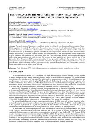
problem of the lid-driven cavity (Rubin and Khosla, 1977; Shankar and Deshpande, 2000), Fig. 1, where u and v are the
velocity components in the x and y directions, respectively. Two formulations are used: streamfunction-velocity and
streamfunction-vorticity. The analyzed parameters are: the number of nodes; the number of inner iterations; the number
of grid levels; and the Reynolds number. For all the studies, uniform grids are used, up to 1025x1025 nodes, with Re =
100, 400 and 1000. Both formulations performances are also compared.
Figure 1. Boundary conditions for the velocities in the lid-driven cavity.
The lid-driven cavity is a classical problem, extensively adopted to validate computational codes involving the
Navier-Stokes equations (Ghia et al., 1982; Shankar and Deshpande, 2000). It presents simple geometry and
configuration, though there are discontinuities in the two upper corners. Numerical results for moderate Reynolds
numbers are commonly found in the literature, using different solution procedures, while only few works show results
for high Reynolds numbers, such as done by Erturk (2009).
This classical problem was also used to the study and improvement of the multigrid method for the Navier-Stokes
equations. Ghia et al. (1982) used the streamfunction-vorticity formulation with a coupled implicit solver, Reynolds
numbers varying from 100 to 10000 and grids as refined as 257x257 nodes. In this case, the use of the multigrid method
was enough to reduce the CPU time by a factor of four, compared to a singlegrid solution. The same formulation was
used by Zhang (2003), to provide comparisons among second, fourth and sixth order approximation functions for the
Finite Difference Method. Vanka (1986) preferred to use the primitive variables for the multigrid method, using as
solver a symmetric coupled Gauss-Seidel method (SCGS), obtaining solutions for grids up to 321x321 nodes. It was
observed that the CPU time increased almost linearly with the number of nodes, as theoretically predicted, but it also
depended on the adopted Reynolds number. For Re = 5000, for example, it was impossible to reduce the residuals to the
desired level, compromising the accuracy of the numerical solution. Yan and Thiele (1998), on other hand, proposed a
modified Full Multigrid scheme (FMG) using V-cycle, in which only the residual is restricted to the coarse grid, unlike
the FAS, which restricts the residual and the solution.
Yan et al. (2007) provided a general verification of the algorithm presented by Yan and Thiele (1998), using high-
order convection schemes, laminar and turbulent 2D and 3D models, several geometries and different types of grids,
providing a comparison among the performances of the modified full multigrid (FMG), the classical FMG and the
singlegrid. The modified FMG presented an expressive performance growth: for the lid-driven cavity, in a 256x256
volumes grid, with Re = 400 and 1000, S = 187 and 169, respectively, for the classical FMG, while for the modified
FMG, S = 289 and 284, in this order. These results, however, corroborates the previous studies of Vanka (1986), once
the speed-up factor slightly reduces with the increasing of the Reynolds number. Kumar et al. (2009) used the primitive
variables formulation, using a high order scheme for the convective terms and a second order scheme for the diffusive
 1,0
 0,1
0=v=u 0=v=u
0=v=u
,=u 1 0=v
y
x

st
ones. It was observed that the number of grid levels did not influence the computational cost. Using a 129x129 nodes
grid, with 4 levels and Re = 1000 and 5000, the obtained speed-up factors were about 10.41 and 8.06 respectively. The
streamfunction-velocity formulation was firstly proposed by Gupta and Kalita (2005), to solve the lid-driven cavity
problem. The accuracy of the numerical solutions was analyzed for grids up to 161x161 nodes and Re = 10000, with
singlegrid. Santiago et al. (2010), using the same formulation, studied the accuracy of the numerical solution for grids
up to 1025x1025, optimizing some parameters of the multigrid method, for Re ≤ 5000.
The next sections of this work presents: the mathematical model (section 2), the numerical model (section 3), the
numerical results and their analysis (section 4) and the conclusions (section 5).
2. MATHEMATICAL MODEL
2.1. Streamfunction-velocity: ψ v
Considering the streamfunction-velocity formulation, the two-dimensional Navier-Stokes equations, for an
incompressible viscous flow, can be reduced to a forth-order partial differential equation (Gupta and Kalita, 2005):






































3
3
2
3
2
3
3
3
4
4
22
4
4
4
2
y
ψ
+
yx
ψ
v+
yx
ψ
+
x
ψ
uRe=
y
ψ
+
yx
ψ
+
x
ψ
(1)
where ψ is the streamfunction, Re is the Reynolds number, and x and y are the spatial coordinates. The velocity
components are defined as
y
ψ
=u


and
x
ψ
=v


 (2)
For all the boundaries, Dirichlet boundary conditions are applied, according to Fig. 1.
2.2. Streamfunction-vorticity: ωψ 
Considering the streamfunction-vorticity formulation, the two-dimensional viscous fluid flow is modeled by the
following equations (Schreiber and Keller, 1983; Erturk, 2009):



















y
ω
x
ψ
x
ω
y
ψ
=
y
ω
+
x
ω
Re2
2
2
2
(3)
ω=
y
ψ
+
x
ψ





2
2
2
2
(4)
where ω is vorticity. Equations (3) and (4) are Poisson-like ones and are coupled by two variables, ψ and ω. The
velocity components are given by Eq. (2).
3. NUMERICAL MODEL
The domain, shown at Fig. 1, is divided into a given number of nodes, N = Nx Ny, where Nx and Ny are related to the
number of nodes in each one of the Cartesian coordinate directions x and y, respectively. Each grid node presents as
coordinates the pair (xi, yi) = ((i – 1)hx, (j –1) hy)), where hx = 1/(Nx – 1) and hy = 1/(Ny – 1) are the grid size elements in
each one of the coordinate directions, and i varies from 1 to Nx, while j varies from 1 to Ny. The partial differential
equations are discretized by the use of the Finite Difference Method (Tannehill et al., 1997), using uniform grids and
second order approximation schemes.
A second order compact scheme (Lele, 1992) was employed for the streamfunction-velocity formulation. In this
scheme, each node (xi, yi) is connected to its eight closer neighbors, resulting in a nine diagonal matrix of coefficients.
The velocity components, Eq. (2), are evaluated using forth order approximation functions, as suggest by Gupta and
Kalita (2005). For the streamfunction-vorticity formulation, the second order central differencing scheme (CDS) is
employed (Tannehill et al., 1997), originating a five diagonal matrix of coefficients. In both formulations, the system of
linear equations originated by the discretization of Eqs. (1), (3) and (4) can be written as

st
hhh
f=φA (5)
where Ah
is a discrete operator, φh
is the numerical solution, f h
is the independent term, and h = hx = hy is the grid
spacing. For refined grids, with small values of h, the system given by Eq. (5) can reach millions of unknowns.
There are two possibilities about the data transfer among grids for the multigrid method. In the first option, only the
residual is transferred, providing the methodology known as Correction Scheme (CS), more appropriated for linear
problems. The second option is the transference of both the residual and the solution, according a methodology known
as Full Approximation Scheme (FAS), more appropriate for non-linear problems (Brandt, 1977). In the present work,
the FAS scheme, associated to the V-cycle and a coarsening ratio of two was adopted for the multigrid method.
In a typical FAS V-cycle, the system of linear equations, in the finest grid, is solved using only few iterations. The
residual, given by Rh
= f h
– Ah
φh
, and the approximated solution are transferred to the nearest coarser grid, in which the
solution is updated with the use of the residual and then some more few iterations are made, providing a new solution
approximation. This process is repeated up to the chosen coarsest grid, in which the correction is interpolated and used
to correct the solution in the immediately finer grid. The system of equations is solved in all the grid levels.
The information transfer process among the grids requires the use of some operators, for both restriction and
prolongation processes. In both cases, literature provides several options, for example: injection, full weighting and half
weighting, for restriction; and bilinear, trilinear and cubic interpolation, for prolongation (Briggs et al., 2000;
Trottenberg et al., 2001). The most used operators, however, are the injection (for restriction) and the bilinear
interpolation (for prolongation). Attention must also be paid to the error smoothing properties: the used solver must
guarantee this property (Trottenberg et al., 2001; Wesseling and Oosterlee, 2001). In the present work, the Successive
Over-Relaxation (SOR) method was adopted as smoother. An outer iteration is characterized by a complete V-cycle,
while the inner iteration is concerned about the smooth iteration carried out in the SOR method in any grid level.
3.1. Streamfunction-velocity: ψ v
In this formulation, there is only one system of linear equations to be solved with the multigrid method. Both the
residual and the approximated solution were transferred by a full weighting (in the restriction) and interpolated by the
bilinear operator (prolongation), because the use of injection for the restriction process caused the divergence for all the
tests. Each inner iteration of the SOR solver was over-relaxed by a parameter λ Î(0;1.4). The best results, based on
numerical tests, was obtained with ν = 1 in the finest grid and ν = 20 in the coarsest grid. In the end of each V-cycle, the
convergence process is checked, based on the ratio between the infinity norm evaluated in the k iteration and the same
norm evaluated in the first iteration. The iterative process was interrupted when
71
10/ 

RRk
(6)
where Rk
is the residual of ψ in the k iteration, and R1
is the residual in the first iteration. The velocity components were
updated only in the finest grid, using the numerical approximations of Eq. (2), the TDMA method and the boundary
conditions specified in Fig. 1; ψ = 0 was employed as initial guess for the calculations.
3.2. Streamfunction-vorticity: ωψ 
In this formulation, there are two Poisson-like equations, which provide two systems of linear equations: one
associated to the vorticity and the other one, to the streamfunction. Both the residual and the approximated solution
were transferred by injection (in the restriction) and interpolated by the bilinear operator (prolongation), once the use of
full weighting for the restriction process caused the divergence for all the tests. Each inner iteration of the SOR solver
was sub-relaxed by a parameter λ Î(0;1); a reduction of about 5% was observed in the CPU time in some intermediate
grids, when there was no relaxation for the streamfunction. There is a coupling between ψ and ω, clearly seen in Eqs.
(3) and (4); in this case, the vorticity solution is used as a source-term to evaluate the streamfunction in the iterative
process. From numerical results, it was observed that ν = 1, in the finest grid, was the best choice for both vorticity and
streamfunction equations.
At the boundaries, the vorticity is evaluated only for the finest grid according the second-order Jensen formula
(Erturk, 2009; Chen et al., 2008), given by
hh
+ψψψ
=ω cc
c
3u
2
87
2
21


(7)
where the indices: c denotes a node on the boundary, 1 the adjacent node to the boundary (neighbor to c) and 2 the node
in the second line adjacent to the boundary (neighbor to 1). The velocity components were evaluated in a post-

st
processing step, using numerical approximations of Eq. (2), the TDMA method and boundary conditions specified in
Fig. 1. The initial guesses are ψ = ω = 0 and the iterative process is interrupted when the following criterion is achieved
  711
10//max 

ω
k
ωψ
k
ψ RR,RR (8)
where Rk
is the residual in the k iteration, R1
is the residual in the first iteration, and the index is related to the variable.
According to Ghia et al. (1982), the use of traditional iterative methods to solve the discrete systems associated to
the Navier-Stokes equations leads to very low convergence rates, which are, in general, dependent on parameters as the
Reynolds number and the grid refinement. Even when the multigrid method is used, some numerical results (not
presented in this work) show that both the Gauss-Seidel and the Modified Strongly Implicit (MSI) (Schneider and
Zedan, 1981) methods are extremely slow, with worse performances for higher Reynolds numbers.
4. RESULTS
Numerical multigrid codes were implemented using Fortran 95 language. The simulations were done in desktop
computer, with an Intel Core 2 Duo processor, 2.66 GHz and 8 GB RAM, using one core. For each formulation, about
300 simulations were done to evaluate the effects, on the CPU time, of the number of inner iterations (ν), the number of
grid levels (L), the size of the problem (N) and the Reynolds number (Re). The optimum value of a parameter is defined
as the value which presents the minimum CPU time, when the other parameters are kept constant; in this case, νoptimum is
the optimum number of inner iterations, while Loptimum is the optimum number of grid levels.
In the ψ-v formulation, a strong sub-relaxation (λ = 0.001) was necessary for the 65x65 nodes grid, with Re = 1000;
in all the other simulations of this formulation, the value of λ = 1.3 was adopted. Gupta and Kalita (2005) also reduced
the relaxation parameter for high Reynolds numbers and coarser grids; the adopted solver, however, was the Bi-
Conjugated Gradient Stabilized method (BiCGStab) (Burden and Faires, 2003). In the ψ-ω formulation, for Re = 100,
the value of λ = 0.8 for almost all grids. Smaller values of λ were employed for coarser grids with high Reynolds
numbers: for example, for Re = 1000, in the 1025x1025 nodes grid, λ = 0.8 was enough to guarantee the numerical
solution convergence; this value, however, was gradually reduced, reaching 0.02 for the 65x65 nodes grid.
4.1. Inner iterations ( ν )
The effect of the number of inner iterations (ν) was analyzed for the grids with N = 65x65, 129x129, 257x257,
513x513 and 1025x1025 nodes and Re = 100, 400 and 1000. The influence of ν on the CPU time is shown in Fig. 2 for
(a) Re = 100, (b) Re = 400 and (c) Re = 1000; the value of ν, which provides the minimum CPU time, is indicated with a
"star" symbol (*).
In the ψ-v formulation, there is not a unique value for νoptimum: for Re = 100 and 400 (Figs. 2a and 2b), νoptimum
increases with the grid refinement (increasing of the number of nodes), while for Re = 1000 (Fig. 2c) this behavior is
not observed. The CPU time behavior, for Re = 100 (Fig. 2a), was similar to the one observed by Santiago and Marchi
(2008) for two-dimensional models: Navier, Burgers (coupled) and Laplace equations; there was no convergence,
however, when ν < νoptimum for Re = 100. Another important remark is the sensitivity of ν to the Reynolds number and
the grid refinement, especially for Re > 100 (Figs. 2b and 2c).
In the ψ-ω formulation, excepted by the 65x65 nodes grid, νoptimum = 4 for Re = 100 (Fig. 2a). For the other
Reynolds numbers, however, this was not the observed behavior. For Re = 400 (Fig. 2b), νoptimum = 4 for the 257x257
nodes grid, while for both the 65x65 and 129x129 nodes grid, νoptimum = 5 (the use of ν = 4 implied in an increment of
about 5% in the CPU time). And for Re = 1000 (Fig. 2c), νoptimum = 4 for the 65x65 and 513x513 nodes grids and νoptimum
= 2 for the 129x129, 257x257 and 513x513 nodes grids. It must be noted that, for this formulation, except by the 65x65
nodes grid with Re = 100, there was no convergence when ν > νoptimum.
4.2. Number of grid levels (L)
The influence of the number of grid levels (L) on the CPU time was studied using grids with N = 129x129, 257x257
and 513x513 nodes, Re = 100, 400 and 1000 and the νoptimum values obtained in the previous section. For each grid, L
could assume values in the range 1 ≤ L ≤ Lmaximum, being L = 1 correspondent to the singlegrid method and L = Lmaximum,
to the use of all the possible auxiliary grids, with the coarsest grid presenting only one internal node. For example, for
the grid 513x513, the auxiliary grids are 257x257, 129x129, 65x65, 33x33, 17x17, 9x9, 5x5 and 3x3, totalizing (with
the finest grid) Lmaximum = 9 grids.
Figure 3 presents the numerical results about the influence of L on the CPU time; the value of L, which provides the
minimum CPU time, is indicated with a "star" symbol (*). In the ψ-v formulation, for Re = 100 (Fig. 3a), numerical
results corroborate previous analyses made for other problems (Santiago and Marchi, 2008; Pinto and Marchi, 2007):
Loptimum = Lmaximum, in other words, the minimum CPU time was obtained with the use of all possible auxiliary grids. The
use of smaller values of L implies in an increment of the CPU time, which can be small, of about only 5%, when L =

st
Lmaximum – (1 to 4), or significant, when an even smaller number of auxiliary grids is employed. Similar behavior is
observed for Re = 400 (Fig. 3b) and Re = 1000 (Fig. 3c). The CPU time increment, when L > Lmaximum – (1 to 4),
however, is smaller than the observed for Re = 100. The use of more refined grids (513x513 nodes) seems to expand the
range in which the CPU time is not much affected by the choice of L once, for Re = 400 and 1000, only a tiny variation
of the CPU time (smaller than 3%) is observed for L > Lmaximum – (1 to 6); in the coarser grid (129x129 nodes),
nevertheless, the choice of Loptimum = Lmaximum is more obvious, for Re = 1000.
Figure 2. Effect of the number of inner iterations on the CPU time.
In the ψ-ω formulation, there is an independence of the CPU time about the adopted Reynolds number. In all the
cases, again, Loptimum = Lmaximum. The CPU time increment, when L > Lmaximum is more expressive than the observed for
the ψ-v formulation: taking the 513x513 nodes grid, for example, and using L = Lmaximum – (1 to 3), the CPU time grows
9.5% for Re= 100 and 10% for Re = 1000 (remembering that this values were about 3 to 5% for the previous
formulation).
All the conclusions for L obtained in this work are consistent on other results presented in the literature: Pinto and
Marchi (2006) recommend the use of L = Lmaximum for the Laplace equation, while for this same problem Tannehill et al.
(1997) showed that the computational effort using L = 4 or 5 was practically the same of using L = Lmaximum, for a
129x129 nodes grid. Otherwise, Rabi and De-Lemos suggest the use of at least 4 levels in solving the two-dimensional
advection-diffusion problem. Qualitatively, this work presents an excellent agreement to the behavior shown by Pinto
and Marchi (2006) for the two-dimensional Laplace equation and by Santiago and Marchi (2007) for the two-
dimensional Laplace and Navier equations, even if another problem (Navier-Stokes equations), with alternative
formulations and the FAS scheme are employed.
4.3. Size of the problem (N)
In this section, the values of νoptimum and Loptimum found in the previous ones are employed. Grid sizes varies from N =
17x17 nodes up to N = 129x129 for the ψ-v formulation, and up to N = 513x513 for the ψ-ω one, using the singlegrid
method. This limitation is associated to the fact that the CPU time increases fast with the growth of N. For coarser grids,

st
it was not possible to obtain numerical solutions for Re = 400 and 1000 and, using the multigrid method, numerical
results were obtained to grids with up to N = 1025x1025 nodes, for both formulations.
Figure 3. Effect of the number of levels on the CPU time.
The CPU time behavior, using both the multigrid and the singlegrid methods, is shown at Fig. 4: the more refined
the grid is, the more advantageous is the use of the multigrid, in agreement with Ferziger and Peric (2001). Such
behavior is more visible for the ψ-v formulation (Fig. 4a): taking the 65x65 and 129x129 nodes grids, for example, the
speed-up's (S) for the multigrid method are S = 203 and S = 60 (for Re = 100 and 400, respectively), for the former grid,
and S = 1543 and S = 185 (for Re = 100 and 400, respectively), for the later grid. These results, furthermore, show the
reduction of the speed-up with the growth of the Reynolds number (for N = 129x129 and Re = 1000, S = 69) and agree
with the observations of Vanka (1986) and Yan et al. (2007).
Another observation for the ψ-v formulation (Fig. 4a) is the absence of proportionality between the growths of the
computational effort and the number of grid nodes (represented by N). For example, for Re = 100, when the N doubles
in each direction, from N = 129x129 to N = 257x257, CPU time increases 8 times, while this variation is of about 9.6
times for the next grid refinement, N = 257x257 to N = 513x513. Similar behavior is observed for other Reynolds
numbers: for Re = 400, these augments are of about 14 and 7.5, for the same grid refinements, and for Re = 1000, the
found values of these growths are 22.7 and 3.6, respectively.
For the ψ-ω formulation (Fig. 4b), although the CPU time associated to the multigrid method is smaller than the
obtained with the use of the singlegrid, the speed-up values are really small and almost constant, for N > 65x65 nodes.
For example, S = 4 for Re = 100 and N = 129x129 nodes, while S = 6 for N = 513x513, keeping the same Reynolds
number, and S = 5 for Re = 1000 and N = 513x513 nodes. These results are similar to the ones obtained by Ghia et al.
(1982), who used the same formulation.
Comparing both formulations, the ψ-ω one presents, in general, the smaller CPU times. This analysis does not count
on the values of the speed-up, once for each formulation, the CPU time associated to the singlegrid method is different,
with much higher values observed to the ψ-v formulation.

st
The text-book performance of the multigrid method is observed for some two-dimensional problems, such as the
Laplace, Navier and Burgers equations (Tannehill et al., 1997; Santiago and Marchi, 2007). However, for two-
dimensional flows, governed by the Navier-Stokes equations, and using primitive variables, the multigrid performance
is much smaller, as observed by Ferziger and Peric (2001). This performance reduction could be associated to the
pressure-velocity coupling, existent in the primitive variables formulation. Using alternative formulations, however, this
coupling effect does not exist any more. The numerical results presented in this work, for both the ψ-v and the ψ-ω
formulations, nevertheless, show the same performance degeneration and agree with Ghia et al. (1982) results. Based
on this, it is likely to attribute the performance degeneration of the multigrid method, for the Navier-Stokes equations,
mainly to the physics of the problem; other factors, including the mathematical formulation and the multigrid
parameters, seem to have a secondary role.
Figure 4. Multigrid performance compared to the singlegrid one for both formulations.
5. CONCLUSION
The two-dimensional incompressible flow in the lid-driven cavity was solved using two alternative formulations
(streamfunction-velocity and streamfunction-vorticity), in order to analyze the influence of the chosen formulation on
the geometric multigrid performance. Some multigrid parameters were also studied: the number of inner iterations (ν)
and the number of grid levels (L), for different Reynolds numbers (Re) and different grid sizes (N). The chosen
multigrid method includes: FAS scheme, V-cycle and refinement ratio equals to 2. For both formulations, the
differential equations were discretized by the Finite Difference Method, with second order central differencing
approximations and uniform grids. The systems of linear equations were smoothed using the SOR method.
As main results, it was verified that:
1) The CPU time is strongly influenced by the adopted values of ν, L, N and Re.
2) νoptimum is not the same for all the grids and varies with N and Re, beyond its dependence on the adopted formulation.
3) Usually, Loptimum = Lmaximum.
4) For the same values of N and Re, the ψ-ω formulation presents, in general, the smaller CPU time values.
5) The degeneration of the multigrid performance observed for the Navier-Stokes equations seems to be related mainly
to the physics of the problem; other factors, such as the mathematical formulation and the multigrid parameters,
seem to have a secondary role.
6. ACKNOWLEDGEMENTS
The first author would like to acknowledge the Laboratory of Numerical Experimentation (LENA) of the
Department of Mechanical Engineering (DEMEC), the Federal University of Paraná (UFPR) and the Federal
Technology University of Paraná (UTFPR) by the physical support provided to the conclusion of this work. The second
author is supported by a scholarship by CNPq (Conselho Nacional de Desenvolvimento Científico e Tecnológico,
Brazil). The authors would like to acknowledge, also, the financial support provided by CNPq, CAPES (Coordenação
de Aperfeiçoamento de Pessoal de Nível Superior, Brazil), Fundação Araucária (Paraná, Brazil) and the Brazilian Space
Agency (AEB), by the UNIESPAÇO Program.

st
7. REFERENCES
Botella, O. and Peyret, R., 1998, “Benchmark spectral results on the lid-driven cavity flow”, Computers & Fluids, Vol.
27, pp. 421-433.
Brandt, A., 1977, “Multi-Level adaptive solutions to boundary-value problems. Mathematics of Computation”, Vol. 31,
No.138, pp. 333-390.
Briggs, W.L., Henson, V.E. and McCormick, S.F., 2000, “A Multigrid Tutorial”. 2nd Ed., SIAM.
Burden, R.L. and Faires, J.D., 2003, “Análise Numérica”, Ed. Pioneira Thomson Learning, São Paulo, Brasil.
Chen, S., Tolke, J. and Krafczyk, M., 2008, “A new method for the numerical solution of vorticity-streamfunction
formulations”, Computer Methods in Applied Mechanics and Engineering, Vol. 198, pp. 367–376.
Erturk, E., 2009, “Discussions on driven cavity flow”, International Journal for Numerical Methods in Fluids; Vol. 60,
pp. 275–294
Ferziger, J.H. and Peric, M., 2001, “Computational Methods for Fluids Dynamics”. 3rd ed., Springer.
Fortuna, A. O., 2000, “Técnicas Computacionais para Dinâmica dos Fluidos”, Edusp, São Paulo, Brasil.
Fox, R.W., McDonald, A.T., 1995, “Introdução à Mecânica dos Fluidos”, Guanabara Koogan, Rio de Janeiro, Brasil.
Ghia, U., Ghia, K.N. and Shin, C.T., 1982, “High-Re solutions for incompressible flow using the Navier-Stokes
equations and a multigrid method”, Journal of Computational Physics, Vol. 48, pp. 387-411.
Gupta, M.M. and Kalita, J.C., 2005, “A new paradigm for solving Navier-Stokes equations: streamfunction-velocity
formulation”, Journal of Computational Physics, Vol. 207, pp. 52-68.
Hackbusch, W., 1985, “Multi-Grid Methods and Applications”, Springer-Verlag, Berlin.
Kumar, D.S., Kumar, K.S. and Das, M.K., 2009, “A fine grid solution for a lid-driven cavity flow using multigrid
method”, Engineering Applications of Computational Fluid Mechanics, Vol 3, No. 3, pp. 336-354.
Lele, S.K.,1992, “Compact finite difference schemes with spectral-like resolution”, Journal of Computational
Physics,Vol. 103, pp. 16-42.
Pinto, M.A.V. and Marchi, C.H, 2006, “Efeito de parâmetros do método multigrid CS e FAS sobre o tempo de CPU
para a equação de Laplace Bidimensional”, Proceedings of the 11th Brazilian Congress of Thermal Sciences and
Engineering (ENCIT), Curitiba, Brazil.
Pinto, M.A.V. and Marchi, C.H, 2007, “Optimum parameters of a geometric multigrid for the two-dimensional
Laplace’s equation”, Proceedings of 19th International Congress of Mechanical Engineering (COBEM), Brasília,
Brazil.
Rabi, J.A. and DeLemos, M.J.S., 2001, “Optimization of convergence acceleration in multigrid numerical solutions of
conductive-convective problems”, Applied Mathematics and Computation, Vol. 124, No. 2, pp. 215–226.
Rubin, S.G. and Khosla, P.K., 1977, “Polynomial Interpolation Methods for Viscous Flow Calculations”, Journal of
Computational Physics, Vol. 24, pp. 217-244.
Santiago, C.D. and Marchi, C.H., 2007, “Optimum parameters of a geometric multigrid for a two-dimensional problem
of two-equations”, Proceedings of 19th International Congress of Mechanical Engineering (COBEM), Brasília,
Brazil.
Santiago, C.D. and Marchi, C.H, 2008, “Parâmetros ótimos do método multigrid geométrico CS e FAS para problemas
2D com duas equações”, Proceedings of XXIX Iberian Latin American Congresso in Computational Methods in
Engineering (CILAMCE), Maceió, Brazil.
Santiago, C.D. , Marchi, C.H. and Souza, L.F., 2010, “Análise do desempenho do método multigrid geométrico com a
formulação função de corrente e velocidade”, Anais do VI Congresso Nacional de Engenharia Mecânica
(CONEM), Campina Grande, Paraíba.
Schneider, G.E. and Zedan, M., 1981, “A Modified Strongly Implicit Procedure for Numerical Solution of Field
Problems”, Numerical Heat Transfer, Vol. 4, pp. 1-19.
Schreiber, R. and Keller, H.B., 1983, “Driven cavity flows by efficient numerical techniques”, Journal of
Shankar, O.N. and Deshpande, M.D., 2000, “Fluid mechanics in the driven cavity”, Annual Review of Fluid
Mechanics, Vol. 32, pp. 93–136.
Tannehill, J.C., Anderson, D.A. and Pletcher, R.H., 1997, “Computational fluid mechanics and heat transfer
Washington”, Taylor & Francis, 2 Ed.
Trottenberg, U., Oosterlee C. W. and Schüller A., 2001, “Multigrid”. Academics Press.
Vanka, S.P., 1986, “Block-Implicit Multigrid Solution of Navier-Stokes Equations in Primitive Variables”, Journal of
Wesseling, P. and Oosterlee, C. W., 2001, “Geometric Multigrid with Applications to Computational Fluid Dynamics”,
Journal of Computation and Applied Mathematics, Vol. 128, pp. 311-334.
Yan, J. and Thiele, F. 1998, “Performance and accuracy of an modified full multigrid algoritm for fluid flow and heat
transfer”. Numerical heat transfer, Part B, Vol 34, pp. 323-338.
Yan, J., Thiele, F. and Xue L. 2007, “A modified full multigrid algorithm for the Navier-Stockes equations”. Computer
& Fluids Vol. 36, pp. 445-454.

st
Zhang , J., 2003 , “Numerical Simulation of 2D Square Driven Cavity Using Fourth-Order Compact Finite Difference
Schemes”, Computers and Mathematics with Applications, Vol. 45, pp. 43-52.
8. RESPONSIBILITY NOTICE
The authors are the only responsible for the printed material included in this paper.

2011 santiago marchi_souza_araki_cobem_2011

Recommended

Recommended

More Related Content

What's hot

What's hot (17)

Viewers also liked

Viewers also liked (13)

Similar to 2011 santiago marchi_souza_araki_cobem_2011

Similar to 2011 santiago marchi_souza_araki_cobem_2011 (20)

Recently uploaded

Recently uploaded (20)

2011 santiago marchi_souza_araki_cobem_2011