1. Heat Transfer study on Numerical Analysis Methodology
Jesse Thomas
4/3/15
Introduction:
The transfer of thermal energy along temperature gradients is the basis of heat transfer. Described
mathematically with the combined heat equation, real objects can be simulated and the heat transfer
anticipated. It is the application of linear algebra and numerical methods that allows engineers to draw
conclusions between simulations and complex geometries or initial conditions.
This report explores the heat equation in three dimensions using the vector matrix capabilities of
MatLab. The simulated object is a long, rectangular bar with cross-sectional dimensions of 100mm x
150mm with uniform temperatures on each side. In this report, the transfer of heat and interactions inside
of the cross-section are investigated using the Gauss-Seidel method of solving linear partial differentiable
equations. The Gauss-Seidel method is also explored in some detail, varying tolerances, resolution and
runtime for the creation of a standardized format for use with the approach.
Method:
The initial conditions used, beginning with side temperatures from the top and clockwise were 75,
60, 85 and 30 degrees C. The initial guess for uniform cross-sectionaltemperature being a hazard of 55
degrees C to begin with. Tolerances were set to Res > 0.0001 and resolution beginning at 9. Throughout
the experiment, all initial conditions were varied to create a robust code and provide a practical standard.
Parting from the initial conditions, the first variable tested was the resolution of the output. To
achieve the initial condition of 9 resolution, Nx and Ny were both initialized at a value of 3. Nx and Ny
were varied from the initial 3 to 31 with a cursory runtime test at 41 and then 51 to test the viability and
effects of very high resolution. Runtime was measured using a digital stopwatch and result quality was
measured by its effect on center node temperature and subjective aesthetics such as smoothness of charted
data. A shortlist of resolutions was recorded for further experimentation for use as the ideal standard.
Using the values Nx=21, Ny=21, the residual tolerance was varied between E-4 and E-5 at
increments of 5E-6 to assess the influence of tolerance on the number of iterative cycles performed by
using the Gauss-Seidel method as well as the responsiveness and runtime of the computations. As a
benchmark of improvement and diminishing returns, previously acquired trends of centralnode
temperature from varied resolution were used to compare results in context. These results were applied to
resolution values on the short list to resolve a practical standard for application to other heat transfer
problems.
Using the identified standard, boundary conditions at the four known surfaces of constant
temperature were changed to test predictable, two dimensional heat transfer problems as well as three
dimensional simulations that could be easily estimated. In this way, the program was verified as robust
and acceptable for application to various heat transfer problems as well as it was provided another
opportunity to examine the standard parameter set for adequate tolerance and resolution.
Results and Conclusions:
The results of experimentation with the grid resolution and number of nodes in the Gauss-Seidel
method of linear differential systems of equations showed that there was a great leap in accuracy in initial
growth of the grid. However,the method of increasing precision by manipulating resolution alone was
demonstrated to be inadequate for a number of reasons. Firstly, an increased number of nodes required a
longer runtime to solve. With an acceptably tight tolerance, very high resolutions took an amount of time
to compute that was untenable. For the purposes of this study, only up to Nx=Ny=51 was attempted at
residual > E-3 because of its consequentially insupportable runtime. Secondly, very high resolution grids
without adequately strict tolerances will show diminishing returns from smaller grids due to the
magnified errors in calculation. An example of comparably high resolution with very low tolerance

2. resulted in a choppy image and unreliable data. As seen in figures 1.1 and 1.2, smooth data with low gap
difference between points effectively show the transfer of heat through the cross-sectional area without a
high load or runtime on the machine.
Figures 1.1 and 1.2: High resolution Gauss-Seidel approximations with medium tolerance produce acceptable results. (Problem
statement initial conditions. Nx=Ny=30).
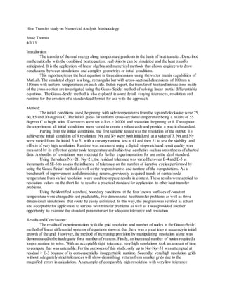
Additional benefits beyond visual evidence due to higher resolution are demonstrated in figure
1.3 which shows the asymptotic approach of the approximation to a true value for center-position nodes
in severalresolutions. It was found that even with very high runtimes upwards of 1.5 minutes (Nx=51),
the precision did not appreciably increase compared to 10 second runtimes at much lower resolutions
(Nx=20) while center node temperature accuracy decreased if tolerance remained constant.
Figure 1.3: Theasymptoticapproach of the Gauss-Seidel method to a truevalue.
Resolutions between Nx=Ny equal to 15 and 21 were recorded for future application as standards.
0
0.02
0.04
0.06
0.08
0.1
0
0.05
0.1
0.15
0.2
30
40
50
60
70
80
90
xy
Temperature
x
y
0.01 0.02 0.03 0.04 0.05 0.06 0.07 0.08 0.09
0.02
0.04
0.06
0.08
0.1
0.12
0.14
62.484
62.486
62.488
62.49
62.492
62.494
62.496
62.498
62.5
62.502
9 25 49 81 121 169 225 289 361 441 529 625 729 841 961
CenterNodeTemperature,C
Grid dimension,Nx*Ny
Center cell temperature(C) corresponding to node field
resolution Nx,Ny

3. The problem of runtime apart from resolution-evoked increase was found to be a consequence of
tighter tolerance. Because the Gauss-Seidel numerical method is asymptotic in nature, a small increase in
tolerance requires many more iterations to converge. By decreasing allowable tolerance by factors of 10
and holding the resolution constant, the relationship in figure 2.1 was discovered.
Figure 2.1: Therelationship between tightened tolerance and the number of iterations of the Gauss-Seidel approximation required
for convergence.
With very loose tolerance at Residual > 10, only two iterations were required while beyond
Residual > 1, many hundreds of iterations were completed before the solution converged. This decrease in
tolerance had an effect on runtime but its linear nature caused the increased calculations to effect runtime
much less than similar increases in the exponentially behavioral resolution property.
Similar to the increased precision due to an increase in resolution, decreased tolerances showed
great initial increases in precision as seen in figure 2.2 but without the loss of accuracy from the high
resolution-loose tolerance example.
2 7
53
162
274
387
499
612
724
837
949
0
100
200
300
400
500
600
700
800
900
1000
10 1 0.1 0.01 0.001 E-4 E-5 E-6 E-7 E-8 E-9
Residual >X
Number of Gauss-SeidelIterations as a Function of
Tolerance, Nx=Ny=21

4. Figure 2.2: increases in solution precision due to tightened tolerance.
Diminishing returns are apparent much earlier in the variance of tolerance which is the
consequence of the limits of Nx=Ny=21 resolution.
More simply explained with respect to numerical analysis: the number of iterations required to
obtain a convergent solution was directly related to the tolerance in the Gauss-Seidel convergence
solution. When allowed a greater tolerance for error, the function discontinued iterations at a solution in
fewer cycles than runs with a more strict tolerance. In figure 2.3 the number of iterations and the core
node temperature (for additional context) have been compared to their respective tolerance values –
Residual > 0.0001 and 0.00001. The difference between the two is that with a tighter tolerance, the
program continued to solve the Gauss-Seidel approximation until the solution was much further on in the
asymptotic approach to a true solution, resulting in more iterations.
55.000 55.008
58.128
62.024
62.452 62.495 62.500 62.500 62.500 62.500 62.500
50
52
54
56
58
60
62
64
10 1 0.1 0.01 0.001 E-4 E-5 E-6 E-7 E-8 E-9
CenterNodeT(C)
Residual >X
Center Node Temperature as a function of Tolerance, Nx=Ny=21

5. Figure 2.3: Iterations required for convergence with respect to tightened tolerances with center node temperatures shown for
context. See figure 2.2 for complete center node temperatureanalysis. (Matlab)
Executing the program using tight tolerances and high resolution was shown to heavily burden
the computer processor resulting, in extreme cases,in computational runtimes up to five or ten minutes
with resolutions only in the few thousands. For this reason, a standard Nx, Ny resolution and tolerances
were identified for comparative and accurate results fit for adequately rigorous analyses. Nx, Ny for this
standard were both held at 21 with a relatively tight tolerance of Residual > E-5. Computational runtime
at this setting on a standard Iowa Engineering machine are within acceptable ranges of 25s to one minute
depending on severalfactors. With this standard, it was possible to vary several important boundary
conditions for comparison and presentation without spending too much downtime in computation and still
providing enough smoothness in data and fidelity to the resolution that inherent variance did not interfere
with side-by-side comparison (e.g. center node temperature at high resolutions and high tolerances).
As an example of the standard chosen above, the boundary conditions and initial temperatures
were reconfigured to Tbottom = 96, Ttop = 15, Tleft = 13, Tright = 55 degrees C. As seen in figures 3.1-
3.4, the smoothness of data with high predictability and resolution provide excellent demonstrations of
heat transfer in three dimensions with a runtime of only 20s in this instance. The experiment and code
was thus shown to be adequately rigorous.
62.497 62.499
222
281
0
50
100
150
200
250
300
350
400
Residual > E-4 Residual > E-5
Iterations and Center Node Temperatureas a function of Gauss-
Seidel tolerance
Center node Temperature (C) Iterations

6. Figures 3.1 and 3.2: Example boundary conditions at standard operating resolution and tolerances (Matlab).
Figures 3.3 and 3.4: Application of the standard developed parameters to a predictable heat transfer problem (Tl=Tr=Tb=0,
Tt=90 C). (Matlab)
Appendix:
Begin Matlab code -
clear all
close all
%Specify grid size
Nx = 21; % you select (and vary) Nx
Ny = 21; % you select (and vary) Ny
%Specify boundary conditions (insert values as per problem assignment)
Tbottom= 0;
0
0.02
0.04
0.06
0.08
0.1
0
0.05
0.1
0.15
0.2
0
20
40
60
80
100
xy
Temperature
0
0.02
0.04
0.06
0.08
0.1
0
0.05
0.1
0.15
0.2
0
20
40
60
80
100
xy
Temperature
x
y
0.01 0.02 0.03 0.04 0.05 0.06 0.07 0.08 0.09
0.02
0.04
0.06
0.08
0.1
0.12
0.14
x
y
0.01 0.02 0.03 0.04 0.05 0.06 0.07 0.08 0.09
0.02
0.04
0.06
0.08
0.1
0.12
0.14

7. Ttop = 0;
Tleft = 0;
Tright = 90;
% initialize coefficient matrix and constant vectorwith zeros
A = zeros(Nx*Ny);
C = zeros(Nx*Ny,1);
% initial ’guess’for temperature distribution (uniform distribution OK -- you specify value)
T(1:Nx*Ny,1) = 55;
% Build coefficient matrix and constant vector
% inner nodes
A = zeros (Nx,Ny);
for n = 2:(Ny-1)
for m = 2:(Nx-1);
i = (n-1)*Nx + m;
%DEFINE COEFFICIENT MATRIX ELEMENTS HERE
A(i,i+Nx) = 1;
A(i,i-Nx) = 1;
A(i,i+1) = 1;
A(i,i-1) = 1;
A(i,i) = -4;
end
end
% Edge nodes
% bottom
for m = 2:(Nx-1)
%n = 1
i = m;
%DEFINE COEFFICIENT MATRIX AND CONSTANT VECTOR ELEMENTS HERE
A(i,i+Nx) = 1;
A(i,i+1) = 1;
A(i,i-1) = 1;
A(i,i) = -4;
C(i) = -Tbottom;
end
%top:
for m = 2:(Nx-1)
% n = Ny
i = (Ny-1)*Nx + m;
%DEFINE COEFFICIENT MATRIX AND CONSTANT VECTOR ELEMENTS HERE
A(i,i-Nx) = 1;
A(i,i+1) = 1;
A(i,i-1) = 1;
A(i,i) = -4;
C(i) = -Ttop;
end
%left:
for n=2:(Ny-1)

8. %m = 1
i = (n-1)*Nx + 1;
%DEFINE COEFFICIENT MATRIX AND CONSTANT VECTOR ELEMENTS HERE
A(i,i-Nx) = 1;
A(i,i+Nx) = 1;
A(i,i+1) = 1;
A(i,i) = -4;
C(i) = -Tleft;
end
%right:
for n=2:(Ny-1)
%m = Nx
i = (n-1)*Nx + Nx;
%DEFINE COEFFICIENT MATRIX AND CONSTANT VECTOR ELEMENTS HERE
A(i,i-Nx) = 1;
A(i,i+Nx) = 1;
A(i,i-1) = 1;
A(i,i) = -4;
C(i) = -Tright;
end
% Corners
%bottomleft (i=1):
i=1;
%DEFINE COEFFICIENT MATRIX AND CONSTANT VECTOR ELEMENTS HERE
A(1,Nx+1) = 1 ;
A(1,2) = 1;
A(1,1) = -4;
C(i) = -(Tbottom + Tleft);
%bottomright:
i = Nx;
%DEFINE COEFFICIENT MATRIX AND CONSTANT VECTOR ELEMENTS HERE
A(i,i+Nx) = 1;
A(i,i-1) = 1;
A(i,i) = -4;
C(Nx) = -(Tbottom + Tright);
%top left:
i = (Ny-1)*Nx + 1;
%DEFINE COEFFICIENT MATRIX AND CONSTANT VECTOR ELEMENTS HERE
A(i,i-Nx) = 1;
A(i,i+1) = 1;
A(i,i) = -4;
C(i) = -(Ttop + Tleft);
%top right:
i = Nx*Ny;
%DEFINE COEFFICIENT MATRIX AND CONSTANT VECTOR ELEMENTS HERE
A(i,i-Nx) = 1;

9. A(i,i-1) = 1;
A(i,i) = -4;
C(i) = -(Ttop + Tright);
%Solve using Gauss-Seidel
residual = 100; % set residual to a big number so loop executes at least once
iterations = 0; % set the iteration counterto zero
while (residual > .000001) % The residual criterion is 0.0001 in this example
% You can test different values
% increment the iteration counter
iterations = iterations+1;
%Transfer the previously computed temperatures to an array Told
Told = T;
%Update estimate of the temperature distribution
%INSERT GAUSS-SEIDEL ITERATION HERE
% Transfer the previously computed temperatures to an array Told
for n=1 : Ny
for m=1 : Nx
i = (n-1)*Nx + m;
Told(i) = T(i);
end
end
% iterate through all of the equations
for n=1 : Ny
for m=1 : Nx
i = (n-1)*Nx + m;
%sum the terms based on updated temperatures
sum1 = 0;
for j=1 : i-1
sum1 = sum1 + A(i,j)*T(j);
end
%sum the terms based on temperatures not yet updated
sum2 = 0;
for j=i+1 : Nx*Ny
sum2 = sum2 + A(i,j)*Told(j);
end
% update the temperature for the current node
T(i) = (1/A(i,i)) * (C(i) - sum1 - sum2);
end
end
%compute residual
% deltaT is a vectorof differences
deltaT = abs(T - Told);
residual = max(deltaT);
end
iterations % report the number of iterations that were executed
%Now transform T into 2-D network so it can be plotted.
delta_x = .100/(Nx+1) % Lx is the width of the bar (insert value)
delta_y = .150/(Ny+1) % Ly is the height of the bar (insert value)
for n=1:Ny
for m=1:Nx
i = (n-1)*Nx + m;
T2d(m,n) = T(i);

10. x(m) = m*delta_x;
y(n) = n*delta_y;
end
end
T2d
% plotting the transpose T2d correctly aligns with x and y vectors
surf(x,y,T2d)
xlabel('x')
ylabel('y')
zlabel('Temperature')
figure
contour(x,y,T2d)
xlabel('x')
ylabel('y')