This document provides an introduction to groupoids. It begins with basic definitions of groupoids, including their partially defined multiplication and inverse properties. It introduces concepts like the unit space, range and source maps. Properties of these concepts are proved, including that the range and source maps are retractions onto the unit space. The document defines topological groupoids and notes they are usually assumed to be locally compact Hausdorff. It provides examples of how groupoids generalize groups, sets, equivalence relations and transformation groups.

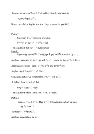
![the fact that r is continuous we have r(ui) → r(u). However, r is a
retraction onto G(0) by Proposition 1.5 so r(ui) = ui. It follows that ui → r(u).
Since G is Hausdorff u = r(u) ∈ G(0) and G(0) is closed. Finally, suppose
(γi, ηi) ∈ G(2) and (γi, ηi) → (γ, η). Then we have γi → γ and ηi → η.
It follows that s(γi) → s(γ) and
r(ηi) → r(η). However, s(γi) = r(ηi) for all i, and
G is Hausdorff so s(γ) = r(η) and (γ, η) ∈ G(2).
An important class of groupoids are those for which the unit spaceis also open.
We will see later that they are very rigid objects with some nice properties.
Definition 1.11.
SupposeG is a locally compact Hausdorff groupoid. If G(0) is open
in G then we say that G is an r-discrete groupoid.
Remark 1.12.
We are using the older definition of r-discrete as given in [Ren80].
However, this definition has fallen out of favor. Currently r-
discrete groupoids are
those for which the unit spaceis open and the range map is a local homeomorph
im.
These groupoids are also called etal´e groupoids. We will see in Proposition 1.2
9
That this is equivalent to assuming that the groupoid is rdiscrete, in the classical
sense,and has a Haar system.Groupoids are very general objects and extend a nu
mber of well understood structures.
The following examples show how groupoids generalize groups, sets, equivale
nce relations, and transformation groups.
Example 1.13.](https://image.slidesharecdn.com/digitaltext-180204134308/85/Digital-text-10-320.jpg)
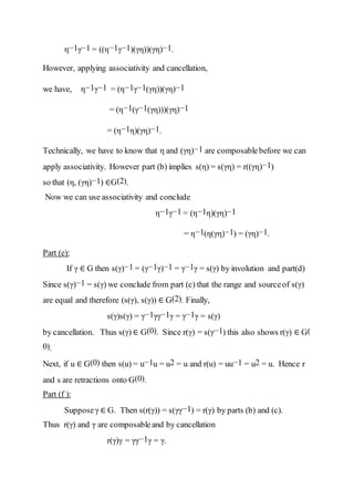
![Then define G(2) = {((x, n, y), (w, m, z)) ∈ G × G : y = w}
and give G the operations (x, n, y)(y, m, z) := (x, n + m, z),
(x, n, y)−1 := (y, −n, x).
With these operations G is a groupoid with unit space G(0) = {(x, 0, x) ∈ G : x ∈
X}.
We usually make the obvious identification of G(0) with X. Under this
identification r(x, n, y) = x and s(x, n, y) = y. Furthermore, in these
circumstances G carries a topology making it into a locally compactHausdorff
r-discrete groupoid [Dea95,Theorem 1] This is known as the “Deaconu-
Renault groupoid” associated to (X, σ).
Example 1.20.
Suppose E = (E0, E1, r, s) is a row-finite2 directed graph without
sources. Let E∞ denote the infinite path spaceof E. Two paths α, β ∈ E∞ are shi
ft
equivalent with lag n ∈ Z, denoted α ∼n β, if there exists N ∈ N such that αi = β
i+nfor all i ≥ N . Let G = {(α, n, β) ∈ E∞ × Z × E∞ : α ∼n β}.Next, define
G(2) = {((α, n, β), (γ, m, δ)) ∈ G × G : β = γ} and let
(α, n, β)(β, m, δ):= (α, n + m, δ),
(α, n, β)−1 := (β, −n, α).
Then G is a groupoid. The unit spaceG(0) = {(α, 0, α) ∈ G : α ∈ E∞} can be
naturally identified with E∞ and the range and sourcemaps are given by
r(α, n, β) = α
and s(α, n, β) = β. It is shown in [KPRR97, Proposition 2.6] that G
carries a topology making it into a locally compactHausdorff
r-discrete groupoid, called the “graphgroupoid” associated to E.
Remark 1.21.
The reason that the groupoids in Examples 1.19 and 1.20 look so](https://image.slidesharecdn.com/digitaltext-180204134308/85/Digital-text-13-320.jpg)
![similar is that they are bothassociated to generalizations of Cuntz-
Krieger algebras
A directed graph is row finite if each vertex emits at most finitely many edges
.[Dea96, KPRR97].Haar measure is essential to the study of locally compact grou
ps because it allows
one to integrate. We will also want to integrate on groupoids and
to do that we will need the following generalization of Haar measure.
END
1.1.1 The Stabilizer Subgroupoid
One slightly surprising fact is that a groupoid (potentially) contains many differ
ent
groups.
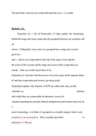
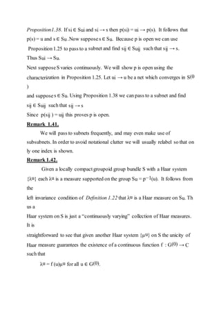
Proposition1.30.
SupposeG is a locally compact Hausdorff groupoid and u ∈ G(0).
Then Su = Gu ∩ Gu = {γ ∈ G : r(γ) = s(γ) = u}, with the operations inherited fro
m
G, is a locally compactHausdorff group which is closed in G.
Proof.
First, it’s clear that u ∈ Su so that Su is not empty. Now, every elem
ent](https://image.slidesharecdn.com/digitaltext-180204134308/85/Digital-text-14-320.jpg)
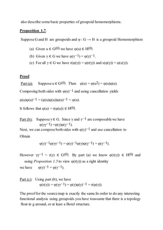
![in Su has range and sourceu so that any two elements are composable. Thus th
e
groupoid operation is everywhere defined on Su × Su and its associative becaus
e ofthe associativity condition in Definition 1.1. Given γ ∈ Su, since s(γ) = r(γ)
= u,we know from Proposition 1.5 that γu = uγ = γ. Finally, given γ ∈ Su we h
aveγ−1γ = s(γ) = u and γγ−1 = r(γ) = u. Thus, Su is a group.
Next supposewe have a net γi → γ in G such that γi ∈ Su for all i. The fact
that the range and sourcemaps are continuous implies r(γi) → r(γ) and
s(γi) →s(γ). However, r(γi) = s(γi) = u for all i so clearly, because G is
Hausdorff, r(γ) = s(γ) = u. Thus Su is closed and it follows that the relative
topology on Su is locally compactHausdorff [Wil07, Lemma 1.26]. Finally,
since the operations are continuous on G they are continuous on Su. Thus Su is
a locally compact Hausdorff group
These groups will play an important role and are given their own special name.
Definition 1.31.
SupposeG is a groupoid and u ∈ G(0) then the group
Su = {γ ∈ G : s(γ) = r(γ) = u}
is known as the stabilizer subgroup of G at u. The set
S := {γ ∈ G : s(γ) = r(γ)} =Su , u∈G(0)
is called the stabilizer subgroupoid of G. Well use p to denote the restriction of th
e
range (and source) map to S. Oftentimes the word isotropy is used interchangeabl
y
with stabilizer.
Remark 1.32. Since Su is a group we will generally denote elements of Su and S
by
lowercase Roman letters, instead of the Greek letters used to denote generic elem
ents
of G.](https://image.slidesharecdn.com/digitaltext-180204134308/85/Digital-text-15-320.jpg)
![compactHausdorff groupoid S such that the range and source maps are equal.
Wewill denote the range (and source)map by p. We view S as a bundle over S(
0)
with
bundle map p and denote the fibres by Su = p−1(u) for all u ∈ S(0). We say
that Sis an abelian group bundle if Su is an abelian group for all u ∈ S(0).
Remark 1.35.
Groupoid group bundles are different than the kinds of group bundles
one
usually encounters. For instance, groupoid group bundles carry no kind of loc
al
triviality condition and the fibres can and will vary over the basespace.
Furthermore,the injection of the unit spaceinto S always gives a continuous
section of the bundle map
Example 1.36.
Supposewe have a locally compactHausdorff group H and a topological
spaceX. Then we can view S = X × H as a group bundle where the bundle
map is just the projection onto the first factor. In this case the unit spacecan be
identified with X and the groupoid operations are obvious.
It turns out that the existence of a Haar system on a group bundle S is equivalent
to requiring the fibres of S vary “continuously.” In order to make this notion
precise we recall the following from [Wil07, Section H.1].
Definition 1.37.
Let X be an arbitrary topological spaceand C(X) the collection of
all closed subsets of X (including the empty set). Given a finite collection F of
open sets of X and a compactsubsetK of X we define](https://image.slidesharecdn.com/digitaltext-180204134308/85/Digital-text-17-320.jpg)
![U (K; F ) := {F ∈ C(X) : F ∩ K = ∅ and F ∩ U = ∅ for all U ∈ F}.
The collection {U (K; F )} forms a basis for a compactHausdorff topology on
C(X) called the Fell Topology.
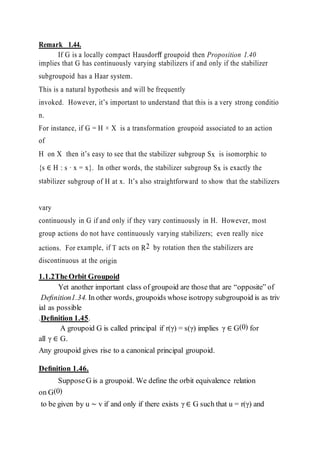
Proposition1.38.
SupposeX is a locally compact spaceand let {Fi}i ∈ I be a net in C(X).
Then Fi → F in C(X) if and only if
(a) given ti ∈ Fi such that ti → t, then t ∈ F , and
(b) if t ∈ F , then there is a subnet {Fij } and tij ∈ Fij such that tij → t.
Using Definition 1.37 to pin down the appropriate notion of continuity we can
make the following
Definition 1.39.
SupposeS is a locally compact Hausdorff group bundle. We saythat S is
continuously varying if given a net {ui} in S(0) such that ui → u in S(0) then
Sui → Su with respectto the Fell topology. If G is a locally compact
Hausdorff groupoid we say that G has continuously varying stabilizers if
its stabilizersubgroupoid S is continuously varying.
At this point we can give some reasonable conditions for the existence of a Haar
system for a group bundle. The following also provides a partial converse to
Proposition 1.24.
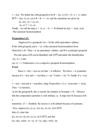
Proposition1.40.
SupposeS is a locally compact Hausdorff groupoid group bundle with
bundle map p. The following are equivalent:
(a) S has a Haar system,
(b) p is open,
(c) S is continuously varying.
Proof.
It is shown in [Ren91, Lemma 1.3] that (a) and (b) are equivalent.
Now supposep is open and ui → u in S(0). We will show Sui → Su using](https://image.slidesharecdn.com/digitaltext-180204134308/85/Digital-text-18-320.jpg)
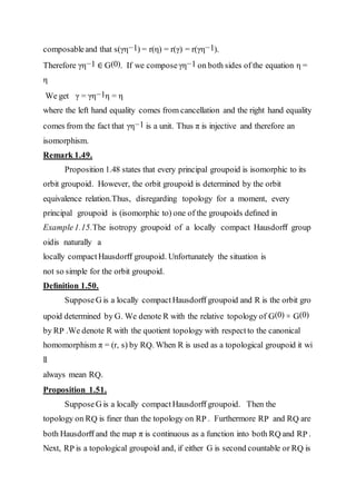
![locally compact,
then RQ is a topological groupoid. Finally, if G has open range
and sourcethen the range and source maps are open as maps on RP and RQ.
Proof.
First we will show π : G → RP is continuous. Supposeγi → γ ∈ G. Sinc
e
the range and source maps are continuous we have (r(γi), s(γi)) → (r(γ), s(γ)) in
G(0) × G(0) and hence in RP . Since RQ has the quotient topology determined
by π, clearly π : G → RQ must be continuous.
Next, supposeO is open in RP , then π−1(O) is open in G, but this implies that
O
is open in RQ. Thus RQ has a finer topology than RP . Furthermore, since any
Subset
of a Hausdorff space inherits a Hausdorff topology, RP is Hausdorff. This
implies RQ is Hausdorff as well, since it carries a finer topology.
It’s pretty easy to see that the operations on RP are continuous with respect
to the product topology. After all (ui, vi) → (u, v) in RP if and only if ui → u a
ndui → u. Proving that the operations are continuous on RQ takes more work, a
nd
more hypotheses. Let I : G → G be defined by I(γ) = γ−1 and consider
π◦I : G → RQ. It’s easy to see that I is a continuous map and that if π(γ) = π(η)
then π ◦I(γ) = π ◦I(η).
Thus I ◦ π factors to a continuous map from RQ into RQ and clearly this
Factorization is nothing more than the inversion operation on RQ. We would
Like to use the Same argument with the multiplication The main issue is the
Following Claim. The map π × π : G × G → RQ × RQ is a quotient map.
Proofof Claim. It is known [Mic68, Section 8] that the product of a quotient m
ap](https://image.slidesharecdn.com/digitaltext-180204134308/85/Digital-text-24-320.jpg)
![with itself need not be quotient. However, there are rather minimal conditions
on RQ which will guarantee that π × π is a quotient map. We know from
[Mic68, Theorem1.5] that if G and RQ × RQ are Hausdorff k-spaces4
then π × π will be a quotient map. It’s clear that G and RQ × RQ are
Hausdorff and, since locally compact spaces are always k-
spaces,all that is left is
to show that RQ × RQ is a k-space.
If, on one
hand, RQ is locally compactthen RQ × RQ is locally compactand we
are done.On
the other hand, supposeG is second countable. Then by choosing a
countable basis of compactneighborhoods we can find a countable collection
{Kn} of compact setswhich cover G and have the property that a set A ⊂ G is
closed if and only if A ∩ Kn is closed for all n.
Such a spaceis known as a kω-space. It follows from [Mic68,Remark 7.5] that
quotients and products of kω-spaces are kω-spaces so that
we can conclude RQ × RQ is a kω-space.
Thus assuming either G is second countable or RQ is locally compact
proves our claim.(2)
RQ × RQ and, since G(2) is just the set of those elements whose range and
sources4A topological space X is called a k-space if a set A ⊂ X is
closed whenever A ∩ K is closed in K for every compactK ⊂ X. Such a
spaceis also called compactly generated.
match up, that G(2) = (π × π)−1(R(2)). It is also straightforward to see that the
restriction of a quotient map to the inverse image of a closed set results in a
quotient (2) be given by M (γ, η) = γη and consider π ◦ M : G(2) → RQ.
Then it’s easy to see that](https://image.slidesharecdn.com/digitaltext-180204134308/85/Digital-text-25-320.jpg)
![if π × π(γ, η) = π × π(γ , η ) then π ◦ M (γ, η) = π ◦ M (γ , η ) so that π ◦ M factor
s
to a operation on RQ implying that composition is continuous.
Finally, supposeG has open range and sourcemaps, that ui → u in G(0) and
that (u, v) ∈ R. First, chooseany γ ∈ G such that π(γ) = (u, v). Since the range
on G is open we can pass to a subnet and find γi → γ such that r(γi) = ui. Then
π(γi) → π(γ) = (u, v) in both RP and RQ and r(π(γi)) = ui. Thus r is open on RP
and RQ. The proofthat s is open is similar.
Remark 1.52.
The astute reader will have noticed that there are several things
missing from Proposition 1.51. For instance, neither RP nor RQ are necessaril
y
locally compact. What’s more, in extreme cases it is not clear if RQ is even a
topological groupoid. On the other hand, the operations on RQ are always
continuous if G is second countable, which includes almost all of the examples
that we will care about. It’s also nice to note that if the topology on RQ is well
behaved (i.e. locally compact)then the operations are continuous then as well.
However, even in this case RQ may not have a Haar system when
G does. Interestingly enough, given a groupoid G there is a duality
between its orbit groupoid and its stabilizer subgroupoid. The following is
stated in [Ren 91,Remark 1.2].
Proposition1.53.
SupposeG is a locally compact Hausdorff groupoid. Then G has
continuously varying stabilizers if and only if the canonical map π = (r, s) is ope
n
onto RQ. Furthermore, under these conditions RQ is a locally compact
Hausdorff groupoid, and if G is second countable then RQ is also.
Proof.](https://image.slidesharecdn.com/digitaltext-180204134308/85/Digital-text-26-320.jpg)

![It follows that RQ is locally compact, since the image of a basis of compact
neighborhoods under π will be a basis of compactneighborhoods for RQ. In th
is
case, Proposition 1.51 implies that the operations on RQ are continuous.
Furthermore,since the image of a countable basis under π will be a countable
basis, if G is second countable then so is RQ.
Remark 1.54.
It is not necessary for the stabilizers to vary continuously for RQ to
be a
locally compactHausdorff (topological) groupoid. Forinstance, consider T
acting on
the closed unit ball in R2 by rotation. Then RQ is compactsince it’s the
continuousimage of a compact space, and is therefore a topological groupoid.
However, the stabilizers are clearly discontinuous at the origin.
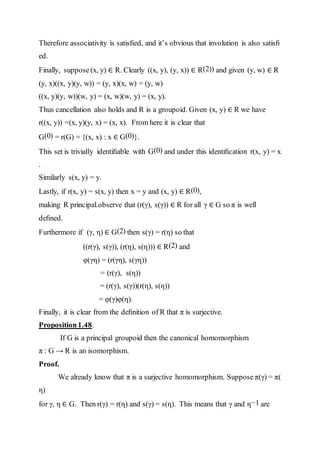
The notion of a groupoid action on a spaceis a straightforward generalization of
group actions. The only caveat is that the action is only “partially defined” in th
e
same sense that the groupoid multiplication is only partially defined. Once agai
n,
much of this section is inspired by [Muh].
Definition 1.55.
SupposeG is a groupoid and X is a set. We say that G acts (on
the left) of X, and that X is a left G-space, if there is a surjection rX : X → G(0)
and
a map (γ, x) → γ · x from G ∗ X := {(γ, x) ∈ G × X : s(γ) = rX (x)} to X such
that
(a) if (η, x) ∈ G ∗ X and (γ, η) ∈ G(2), then (γη, x), (γ, η · x) ∈ G ∗ X and
γ · (η · x) = γη · x,](https://image.slidesharecdn.com/digitaltext-180204134308/85/Digital-text-28-320.jpg)