Modal analysis involves determining the modal parameters of a structure, which describe its inherent dynamic behavior. These parameters include the modal frequencies, damping rates, and mode shapes. A structure's response can be represented as a sum of contributions from individual normal modes of vibration. Each normal mode behaves like a single-degree-of-freedom oscillator and is characterized by its modal parameters. Modal analysis allows constructing a modal model to predict how the structure will respond under various operating conditions.

2. STRUCTURAL TESTING
Part II: Modal Analysis and Simulation
by
Ole Døssing, Brüel&Kjær
Experimental Modal Analysis………………………………. 2
All Structures Exhibit Modal Behaviour………………... 4
Single-degree-of-freedom (SDOF) Models……………….. 6
SDOF Models in the Frequency Domain ...............…...... 7
A Closer Look at Pole Location and Residue .....……..... 9
The DOF and MDOF models ....….................................... 10
What is a Mode Shape? ................................................. 11
Normal Modes and Complex Modes .......................... 12
How Residues Relate to Mode Shapes ...................... 13
Scaling the Mode Shapes .............................................. 14
Modal Coupling ................................................................ 15
What Does the Modal Description Assume? ............ 16
Practical Structures ......................................................... 17
The Lumped-parameter Model and Modal Theory . 18
The Modal Space .............................................................. 19
Specifying the Degrees of Freedom (DOFs) ............ 20
DOFs and the Mobility Matrix ...................................... 22
Modal Test on a Simple Structure .............................. 24
Mode Shapes from Quadrature Picking ..................... 26
Parameter Estimation by Curve-fitting ....................... 28
What is Curve-fitting? ..................................................... 29
Curve-fitters for Modal Analysis .................................. 30
Local and Global Curve-fitters ..................................... 32
Computer-aided Modal Testing ..................................... 33
Step 1 - Setting up the Modal Test .......................... 34
Step 2 - Making the Measurements .......................... 36
Step 3 - Parameter Estimation by Curve-fitting .... 37
Step 4 - Documentation of the Test .......................... 38
The Dynamic Modal Model ............................................ 40
Checking and Applying the Model ............................. 41
Considerations of Model Completeness .................... 42
Computer Simulations .................................................... 43
Response Simulation ...................................................... 44
Modification Simulation .................................................. 46
Applying Modifications ................................................... 47
Implementating Modifications ....................................... 48
Case Story: Application of Synthesized FRFs .....….. 49
Further Reading .............................................................. 51
Symbols and Notation .................................................... 52
March 1988

3. Preface to Part 2
The study of structural dynamics is essential for under-
standing and evaluating the performance of any engineer-
ing product. Whether we are concerned with printed-circuit
boards or suspension bridges, high-speed printer mecha-
nisms or satellite launchers, dynamic response is funda-
mental to sustained and satisfactory operation.
Modal analysis of the data obtained from structural testing,
provides us with a definitive description of the response of
a structure, which can be evaluated against design specifi-
cations. It also enables us to construct a powerful tool, the
modal model, with which we can investigate the effects of
structural modifications, or predict how the structure will
perform under changed operating conditions.
A simplified definition of modal analysis can be made by
comparing it to frequency analysis. In frequency analysis, a
complex signal is resolved into a set of simple sine waves
with individual frequency and amplitude parameters. In
modal analysis a complex deflection pattern (of a vibrating
structure) is resolved into a set of simple mode shapes with
individual frequency and damping parameters.
2
A rigorous mathematical approach to the subject is outside
the scope of this primer. Where necessary we simply quote
the mathematics! definitions required to support our intu-
itive introductions. For readers who need to confirm the
quoted mathematical "truths" we have included a list of rel-
evant literature at the end of this booklet.
To the assumptions already made about the reader (see
preface to part 1), we now add a knowledge of the subject
matter of part 1 (Mechanical Mobility Measurements).

4. Experimental Modal Analysis
Introduction
Most structures vibrate. In operation, all machines, vehicles
and buildings are subjected to dynamic forces which cause
vibrations. Very often the vibrations have to be investigat-
ed, either because they cause an immediate problem, or
because the structure has to be "cleared" to a "standard"
or test specification. Whatever the reason, we need to
quantify the structural response in some way, so that its
implication on factors such as performance and fatigue can
be evaluated.
By using signal-analysis techniques, we can measure vibra-
tion on the operating structure and make a frequency anal-
ysis. The frequency spectrum description of how the vibra-
tion level varies with frequency can then be checked
against a specification. This type of testing will give results
which are only relevant to the measured conditions. The
result will be a product of the structural response and the
spectrum of an unknown excitation force, it will give little or
no information about the characteristics of the structure it-
self.
An alternative approach is the system-analysis technique in
which a dual-channel FFT analyser can be used to measure
the ratio of the response to a measured input force. The
frequency response function (FRF) measurement removes
the force spectrum from the data and describes the inher-
ent structural response between the measurement points.
From a set of FRF measurements made at defined points
on a structure, we can begin to build up a picture of its
response. The technique used to do this is modal analysis.
3

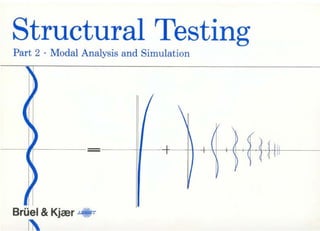
5. All Structures Exhibit Modal Behaviour
An FRF measurement made on any structure will show its
response to be a series of peaks. The individual peaks are
often sharp, with identifiable centre-frequencies, indicating
that they are resonances, each typical of the response of a
single-degree-of-freedom (SDOF) structure. If the broader
peaks in the FRF are analyzed with increased frequency
resolution, two or more resonances are usually found close
together. The implication is that a structure behaves as if it
is a set of SDOF substructures. This is the basis of modal
analysis, through which the behaviour of a structure can be
analyzed by identifying and evaluating all the resonances,
or modes, in its response.
Let us begin with a review of how structural response can
be represented in different domains. Through this we will
be able to see how the modal description relates to de-
scriptions in the spatial, time and frequency domains.
As our example, we will take the response of a bell, which
is a lightly damped structure. When the bell is struck, it
produces an acoustical response containing a limited num-
ber of pure tones. The associated vibration response has
exactly the same pattern, and the bell seems to store the
energy from the impact and dissipate it by vibrating at par-
ticular discrete frequencies.
In the illustration, each column shows the response of the
bell represented in different domains:
In the physical domain, the complex geometrical deflection
pattern of the bell, can be represented by a set of simpler,
independent deflection patterns, or mode shapes.
In the time domain the vibration (or acoustic) response of
the bell is shown as a time history, which can be represent-
ed by a set of a decaying sinusoids.
In the frequency domain, analysis of the time signal gives
us a spectrum containing a series of peaks, shown below
as a set of SDOF response spectra.
In the modal domain we see the response of the bell as a
modal model constructed from a set of SDOF models.
Since a mode shape is the pattern of movement for all the
points on the structure at a modal frequency, a single mod-
al coordinate q can be used to represent the entire move-
ment contribution of each mode.
Looking back from the modal domain, along the rows in the
illustration, we see that each SDOF model is associated
with a frequency, a clamping and a mode shape. These are
the MODAL PARAMETERS:
• modal frequency
• modal damping
• mode shape
which together form a complete description of the inherent
dynamic characteristics of the bell, and are constant wheth-
er the bell is ringing or not.
Modal analysis is the process of determining the modal pa-
rameters of a structure for all modes in the frequency
range of interest. The ultimate goal is to use these parame-
ters to construct a modal model of the response.
Two observations worth noting here are that:
• Any forced dynamic deflection of a structure can be rep-
resented as a weighted sum of its mode shapes.
• Each mode can be represented by an SDOF model.
4

6. 5

7. Single-degree-of-freedom (SDOF) Models
As each peak - or mode - in a structural response can be
represented by an SDOF model, we will look at some as-
pects of SDOF dynamics. In particular, we will examine the
way in which SDOF structure can be modelled in the physi-
cal, time and frequency domains. These models are not in-
tended to represent physical structures, but will serve as
instruments for interpreting dynamic behaviour (constrained
by a set of assumptions and boundary conditions). They will
help us to:
• understand and interpret the behaviour of structures;
• describe the dynamic properties of structures, using a
small set of parameters;
• extract the parameters from measured data (curve-fit-
ting).
•
•
•
• An analytical model can be constructed in the physical
domain. It is an abstract system consisting of a point mass
(m). supported by a massless linear spring (k) and connect-
ed to a linear viscous damper (c). The mass is constrained
so that it can move in only one direction (x) - a Single-
degree-of-freedom.
•
•
•
• A mathematical model in the time domain can be de-
rived by applying Newton's Second Law to the analytical
model. By equating the internal forces (inertia, damping and
elasticity) with the external (excitation) force, we obtain the
model
which is a second-order differential equation. A model
which is more mathematically manageable can be obtained
in the frequency domain.
6

8. SDOF Models in the Frequency Domain
•
•
•
• A spatial-parameter model can be constructed in the
frequency domain to describe the frequency response func-
tion H(ω) in terms of mass, spring stiffness and damping
coefficient.
Let us look at the behaviour of this model under sinusoidal
excitation and see what happens to the magnitude |H(ω)|
and phase as frequency increases.
The static deflection is controlled by spring stiffness alone.
At low frequencies the response is dominated by the spring
and is in phase with the excitation.
As frequency increases, the inertial force of the mass has
an increasing influence. At a particular frequency (ω0 = k/m
the undamped natural frequency) the mass and spring
terms cancel each other out, the response is controlled only
by the damping term, and compliance becomes high. If the
damping term was, in fact, zero the compliance would be
infinite. At ω0, the response lags the excitation by 90°.
At frequencies greater than ω0, the mass term takes con-
trol, the system begins to behave simply as a mass, the
compliance decreases and the response lags the excitation
by 180°.
•
•
•
• The FRF (or black-box) model is non-parametric. It is
based on the definition of H(ω).
X(ω) = H(ω) · F(ω)
H(ω) is in terms of compliance (displacement/force). It is
the ratio of output/input spectra; and varies as a function
of frequency (ω).
This model links the analytical SDOF model to practical
measurements. 7

9. The spatial parameter model is ideal for working with ana-
lytical systems. With real structures we will usually have lit-
tle or no knowledge of the mass, stiffness and damping
distributions. The next model is a practical link between
theory and measurements.
•
•
•
• The modal-parameter model is shown in the illustration.
It is constructed using two parameters which can be ob-
tained from FRF measurements.
In the illustration, H(ω) is defined in terms of the pole loca-
tion (p) and the residue (R) - and their complex conjugates
(p* and R*). The pole location and the residue are them-
selves defined in terms of the spatial parameters.
The pole location is a complex number. The numerical val-
ue of its real part (σ) is the rate at which a damped oscilla-
tion decays. This is shown on the impulse response func-
tion in the time domain. In the frequency domain, a
represents half the -3 dB bandwidth of the FRF peak. The
imaginary part of the pole location is the modal frequency -
the damped natural frequency (ωd) for a free decaying os-
cillation.
The residue for an SDOF system is an imaginary number
which expresses the strength of the mode.
As indicated in the illustration, both the pole location and
the residue can be obtained from measurements made on a
displayed FRF. The modal parameter model thus gives the
relationship between the analytical models and experimen-
tal measurements.
8

10. A Closer Look at Pole Location and Residue
As these two parameters are fundamental to modal analy-
sis, let us look at them in more detail.
•
•
•
• The pole location contains two of the modal parameters
listed on page 4. The real part of the pole location is the
rate at which free vibrations die out (related to the modal
damping), and the imaginary part is the frequency at which
the system oscillates in free decay (modal frequency). This
information is held in the form of a centre frequency and a
half-bandwidth (at -3 dB) of a resonance. The pole location
describes the shape of the magnitude and phase curves of
the FRF. It gives us a qualitative measure of the dynamic
properties.
•
•
•
• The residue is a mathematical concept and has no direct
interpretation in physical terms. It carries the absolute scal-
ing of the FRF, and thus the level of the magnitude curve.
We will see later that the residue is related to the third
modal parameter, the mode shape.
The residue is sometimes called the pole-strength, but the
magnitude of a mode is not given by the residue alone. It is
the ratio of the residue to the decay rate:
R
H(ωd) ≅
σ
The illustration gives an example of the properties of pole
location and residue. In a simplistic SDOF view, a hi-fi turn-
table unit could have the same stiffness, damping and mass
distribution as a car, and hence the same pole location.
Their measured FRFs would have the same shape but their
response to unit force would be quite different. The differ-
ence can be seen in the residues.
9

11. The DOF and Multiple-degree-of-freedom (MDOF) Models
Previous models have been restricted to the SDOF case,
with only one movement in a single direction. Real struc-
tures have many points which can move independently -
many degrees-of-freedom. To make an FRF measurement
on a real structure we have to measure the excitation and
response between two points. But any point may have up to
six possible ways of moving so we must also specify the
measurement direction.
•
•
•
• A degree-of-freedom (DOF) is a measurement-point-and-
direction defined on a structure. An index i is used to indi-
cate a response DOF, and j an excitation DOF. Additional
indices x,y and z may be used to indicate the direction.
Xi(ω)
Thus Hij(ω) ≡ ----------
Fj(ω)
By writing H (ω) in two different ways, we obtain the two
ij
MDOF models shown as equations in the illustration.
•
•
•
• The MDOF FRF-model represents Hij(ω) as the sum of
SDOF FRFs, one for each mode within the frequency range
of the measurement, where r is the mode number and m is
the number of modes in the model.
•
•
•
• The MDOF modal-parameter model defines Hij(ω) in
terms of the pole locations and residues of the individual
modes. This model indicates two significant properties of
the modal parameters:
• Modal frequency and damping are global properties.
The pole location has only a mode number (r) and is
independent of the DOFs used for the measurement.
• The residue is a local property. The index (ijr) relates it
to a particular combination of DOFs and a particular
mode.
10

12. What is a Mode Shape?
A mode shape is, as we said in the bell example on page 4,
a deflection-pattern associated with a particular modal fre-
quency - or pole location. It is neither tangible nor easy to
observe. It is an abstract mathematical parameter which
defines a deflection pattern as if that mode existed in isola-
tion from all others in the structure.
The actual physical displacement, at any point, will always
be a combination of all the mode shapes of the structure.
With harmonic excitation close to a modal frequency, 95%
of the displacement may be due to that particular mode
shape, but random excitation tends to produce an arbitrary
"shuffling" of contributions from all the mode shapes.
Nevertheless, a mode shape is an inherent dynamic proper-
ty of a structure in "free" vibration (when no external forces
are acting). It represents the relative displacements of all
parts of the structure for that particular mode.
•
•
•
• Sampled mode shapes →
→
→
→ the mode shape vector
Mode shapes are continuous functions which, in modal
analysis, are sampled with a "spatial resolution" depending
on the number of DOFs used. In general they are not mea-
sured directly, but determined from a set of FRF measure-
ments made between the DOFs. A sampled mode shape is
represented by the mode shape vector {Ψ}r, where r is the
mode number.
•
•
•
• Modal displacement
The elements Ψir of the mode shape vector are the relative
displacements of each DOF (i). They are usually complex
numbers describing both the magnitude and phase of the
displacement.
11

13. Normal Modes and Complex Modes
Modes can be divided into two classes
• Normal modes
These are characterized by the fact that all parts of the
structure are moving either in phase, or 180° out of phase,
with each other. The modal displacements Ψir are therefore
real and are positive or negative. Normal mode shapes can
be thought of as standing waves with fixed node lines.
• Complex modes
Complex modes can have any phase relationship between
different parts of the structure. The modal displacements Ψir
are complex and can have any phase value. Complex mode
shapes can be considered as propagating waves with no
stationary node lines.
• Where to expect normal/complex modes
The damping distribution in a structure determines whether
the modes will be normal or complex. When a structure has
very light or no damping it exhibits normal modes. If the
damping is distributed in the same way as inertia and stiff-
ness (proportional damping), we can also expect to find
normal modes.
Structures with very localized damping, such as automobile
bodies with spot welds and shock absorbers, have complex
modes.
Warning. The mode shapes derived from poor measure-
ments can indicate complex modes on structures where
normal modes exist.
12

14. How Residues Relate to Mode Shapes
On page 9 we saw that the residue is proportional to the
magnitude of the FRF. At a modal frequency (ωdr) the mag-
nitude is:
It can be shown that the residue for a particular mode (r) is
proportional to the product of the modal displacement Ψir at
the response DOF, and Ψjr at the excitation DOF.
The illustration shows the second mode of a cantilever
beam, with excitation applied at DOF 8, and responses
measured at three DOFs. Notice that the shape of the reso-
nance curve is the same for each measurement, but that
the magnitude is proportional to the modal displacements.
13

15. Scaling the Mode Shapes
The mode shape vector {Ψ}r defines the relative displace-
ment of each DOF, the values of the vector elements Ψir are
not unique.
From FRF measurements we determine the residues, which
do have unique values. The relationship between a residue
and the associated modal displacements, allows us to de-
termine a scaling constant ar for each mode, such that:
Rijr = ar · φir · φjr
where φ and φ are the scaled modal displacements. For a
ir jr
driving-point measurement, this gives us:
Rjjr = ar · φjr
2
The rigorous mathematical approach to modal analysis es-
tablishes a relationship (given in the illustration) between
the mode shape vector {φ}r and the modal mass Mr. If we
apply this to the SDOF case (in which there is only one
displacement and one mass), we can then evaluate ar.
What is the modal mass? The modal mass is not related to
the mass of the structure and cannot be measured. It is
simply a mathematical device which can have any value ex-
cept zero. We can choose its value and then calculate ar.
For simplicity we will work with unit modal mass scaling
(Mr = 1).
Scaled mode shapes. From a driving-point measurement,
we can obtain Rjjr for each mode. By using calculated ar.
values, we can then obtain the scaled driving-point dis-
placements φjr. From the response measurements, we are
then able to scale the values of φir, and produce scaled
mode shapes.
14

16. Modal Coupling
Modal coupling is a general term used to indicate how
much of the response, at one modal frequency, is influ-
enced by contributions from other modes. It can be ob-
served in a displayed FRF around a modal frequency.
•
•
•
• Lightly coupled modes - simple structures
On a lightly damped structure the modes are well separated
and distinct and are said to be lightly coupled. Such struc-
tures behave as SDOF systems around the modal frequen-
cies, and are known as simple structures.
When testing this type of structure, simple methods give
very reliable results. Simple structures are often encoun-
tered in trouble-shooting since most noise, vibration and
fatigue problems are associated with lightly damped reso-
nances.
•
•
•
• Heavily coupled modes - complex structures
On a structure that has heavy damping or high modal den-
sity, the FRFs do not display clearly distinctive modes. The
modes are said to be heavily coupled and the response at
any frequency is a combination of many modes. Complex
structures can still be described using a discrete set of
modes, but the techniques required to determine the modal
parameters are more complicated.
15

17. What Does the Modal Description Assume?
On the previous page we looked at the implications of high
modal density and heavy damping. But neither of these two
factors will prevent us from applying a modal description to
a structure. They merely complicate the techniques re-
quired.
An assumption that we do have to make, however, is linear-
ity.
•
•
•
• Linearity
We have to assume that the systems we test behave linear-
ly so that the response is always proportional to the excita-
tion. This assumption has three implications for Frequency
Response Function (FRF) measurements.
• Superposition. A measured FRF is not dependent on the
type of excitation waveform used. A swept sinusoid will
give the same result as a broadband excitation.
• Homogeneity. A measured FRF is independent of the
excitation level.
• Reciprocity. In a linear mechanical system a particular
symmetry exists which is described by Maxwell's Reci-
procity Theorem. This implies that the FRF measured
between any two DOFs is independent of which of them
is used for excitation or response.
16

18. Practical Structures
In general, structures will behave linearly for small deflec-
tions. But linearity is often violated when deflections be-
come large, so a modal description cannot be used to pre-
dict catastrophic failure.
We must also assume that our structures are:
• Causal. They will not start to vibrate before they are
excited.
• Stable. The vibrations will die out when the excitation is
removed.
• Time-invariant. The dynamic characteristics will not
change during the measurements.
Note. The characteristics of some structures will change
during a test:
The characteristics of a lightweight structure may be
changed by transducer loading.
Over long tests periods, structural characteristics may
be altered by temperature, or other environmental
changes.
Some structures may be changing continuously. The
mass of a flying aircraft, for example, will decrease
gradually as fuel is burned.
17

19. The Lumped-parameter Model and Modal Theory
Much of the theory of modal analysis is based on the math-
ematics of vectors and matrices. In this primer we do not
intend to follow the rigorous mathematical route, but in or-
der to to understand why modal analysis techniques are
valid we need to look at a few theoretical points.
•
•
•
• The lumped-parameter model
This model represents an MDOF structure as a series of
masses, connected together by springs and dampers. By
applying Newton's Second Law we can generate a series of
equations for the motion, one equation for each mass (each
degree of freedom) in the model.
The mathematical way to organize these equations is to use
matrix notation. The mass matrix will contain single mass
values, but the damping and stiffness matrices will have
combinations of values which couple all the equations to-
gether. This coupling indicates that a force applied to one
mass will cause a reaction in all the others, making analysis
of this model complicated.
On a real structure, the mass, damping and stiffness distri-
butions will not usually be known, but we can measure the
pole locations (damping and modal frequencies) and the
residues, and obtain the scaled mode shapes. With these
parameters we can transform the lumped-parameter model
•
•
•
• The modal transformation
If we replace the physical coordinates, in the (matrix) equa-
tion of motion, with the product of the modal matrix (all the
scaled mode shape vectors as columns) and the modal co-
ordinates, we make a transformation into another domain -
the modal space.
18

20. The Modal Space
Transformation into the modal space has a dramatic effect
on the lumped-parameter model. The equations of motion
become decoupled, and can be seen as a collection of in-
dependent SDOF models, one for each mode in the MDOF
model (each modal coordinate).
Each model has a mass of unity (unit modal-mass), a
damping constant equal to the bandwidth of the mode, and
a spring constant equal to the square of the the undamped
natural frequency. The individual models are excited by a
modal force equal to the dot (scalar) product of the mode
shape and the physical force vector (that is, the projection
of the force on the mode shape). The modal force can be
interpreted as the ability of a specific force distribution to
excite a particular mode.
We can now write a set of equations, in terms of the modal
parameters, with solutions in modal coordinates. The equa-
tion for each coordinate can be solved independently as an
SDOF system. When the mode shapes are scaled with unit
modal mass, the equations are in terms of the simple, mea-
surable parameters of natural frequency, modal damping
and scaled mode shape.
19

21. Specifying the Degrees of Freedom (DOFs)
A free point generally has six degrees-of-freedom. Three
translational, and three rotational. No suitable rotational-
transducers are available, but the translational degrees of
freedom are usually sufficient to describe the motion. For
most practical structures, a set of regularly distributed
measurement points in one or two directions is adequate.
•
•
•
• How many DOFs are needed for a test?
The number of DOFs required depends on the purpose of
the test, on the structural geometry, and on the number of
modes in the frequency range of interest.
A test made simply to verify analytically predicted modal
frequencies requires only a few DOFs.
If the purpose of the test is to construct a mathematical
model, then sufficient DOFs must be used for the measured
mode shapes to be mutually orthogonal, or linearly inde-
pendent.
The illustration shows two examples of measurements
made on a rectangular plate, one using four and the other
using thirty DOFs. In the four DOF example, a maximum of
four linearly independent modes are seen. The higher
modes are simply the first four repeated. A model based on
this measurement could only be used up to a frequency
which included the first three or four modes. In the thirty
DOF example, the shapes for the two highest modes are
only roughly represented.
Note. The number of DOFs has to be chosen to represent
the total dynamics of the structure. It is the geometrical
complexity of the mode shapes, rather than to the number
of modes expected, which determines the number of DOFs
required.

22. 21

23. DOFs and the Mobility Matrix
•
•
•
• Input/output combinations
The illustration shows a structure with two defined DOFs,
each of which is an input/output point for an FRF measure-
ment. If we have n defined DOFs, the number of possible
input/output combinations is n x n.
•
•
•
• The mobility matrix
The individual FRF measurements can be arranged as the
elements of a matrix, known as the mobility matrix [H].
Each element Hij(ω) is a particular FRF measurement.
Each row of the matrix contains FRFs with a common re-
sponse DOF. while in each column they have a common
excitation DOF. The diagonal of [H] contains a class of
FRFs for which the response and excitation DOFs are the
same. These are the driving point FRFs. The off-diagonal
elements are transfer FRFs.
22
Note. The term mobility is used in a general sense and may
represent compliance, mobility or accelerance. In models,
[H] generally refers to compliance, but measurements are
usually made in terms of accelerance (see Part 1 Mechani-
cal Mobility Measurements ).
• Minimum sufficient data
The number of DOFs specified in a test can range from ten
to several hundred. The matrix [H] can thus become enor-
mous (when n = 100, [H] contains 10000 FRFs).
Fortunately, reciprocity helps here and all the information
for a linear mechanical structure is contained in either one
complete row, or one complete column of [H]. The number
of measurements needed is therefore equal to the number
of specified DOFs.

24. 23

25. Modal Test on a Simple Structure
To examine the techniques used to extract the modal pa-
rameters, let us look at a modal test on a simple structure,
an example typical of a trouble-shooting problem.
The example given in the illustration can be considered as
a cantilever beam. The simplest instrumentation we can use
is a dual-channel signal analyzer, with hammer excitation,
and an accelerometer to measure the response signal. We
will restrict the investigation to the first few bending modes,
so that four DOFs aligned in the vertical direction will be
sufficient.
Let us assume that the instrumentation has been set up,
preliminary adjustments made, and that a few initial mea-
surements were taken to optimize the frequency range,
weighting functions and input conditioning.
•
•
•
• Determination of pole locations
Any FRF will indicate that the beam has lightly coupled
modes. Therefore structure behaves as a single-degree-of-
freedom system around its modal frequencies, around
which we can assume that all the response is due to that
particular mode.
From any measured FRF we can determine the modal fre-
quencies and dampings, and thus obtain the pole locations.
24

26. • The modal frequencies are determined simply by observ-
ing the maximum magnitudes on the FRF.
• The modal dampings are not so simple to determine,
and will often be the parameters measured with the great-
est degree of uncertainty.
One technique we can use to measure the damping is to
find the -3dB bandwidths. On a lightly damped structure
the resonances are sharp and the peaks are too narrow for
accurate measurements of the bandwidths. This problem
can often be overcome by making a zoom analysis to ob-
tain sufficient frequency resolution for the measurements.
Alternatively we can use a frequency weighting technique,
in which each mode is isolated in turn. Application of both
the Fourier and Hilbert transforms will then give the impulse
response function of the mode. On a display showing loga-
rithmic magnitude of the impulse response function the de-
cay can be seen as a straight line. From this we can find
the time τ taken for the magnitude to decay 8,7 dB. The
decay rate σ is the reciprocal of the decay time, so that
σ = 1/τ.
From these measurements we can find the pole locations,
but we also need to determine the associated mode
shapes.
25

27. Mode Shapes from Quadrature Picking
Remember that the equation for the SDOF model, evaluated
at one of the modal frequencies ωdr, gives us:
With more than one defined DOF we can substitute the resi-
due by:
giving
Notice that A(ω) is an imaginary number at a modal fre-
quency. This gives the basis for the quadrature picking
technique, through which we can determine the mode
shapes.
The FRF appears to become purely imaginary at the modal
frequency. Its amplitude is proportional to the modal dis-
placement, and its sign is positive if displacement is in
phase with the excitation.
The mode shapes can be determined if we fix a response,
or an excitation DOF as a reference and then make a set of
measurements. The imaginary parts of the measured FRFs
can be "picked" at the modal frequencies at which they
represent the modal displacement for that specific DOF.
In our example DOF # 2 is used as the response reference.
A set of FRFs is then measured by exciting each of the four
defined DOFs in turn.
The four imaginary parts of the FRF for each modal fre-
quency represent the associated mode shape. If the mea-
surements were made with calibrated instrumentation, the
mode shapes could then be scaled.
But since our measurements are in accelerance we need to
make a double differentiation to produce an accelerance
model:
26

28. 27

29. Parameter Estimation by Curve-fitting
In the previous example the modes were lightly coupled, we
determined the modal parameters simply by picking a num-
ber of discrete values from the FRF measurements.
When the measured data indicates heavily coupled modes
or noise contamination, or when high accuracy is required
for the estimation, we can make a computer-aided modal
analysis. A curve-fitting technique can then be used to im-
prove the modal parameter estimation.
•
•
•
• Gold in ⇒
⇒
⇒
⇒ gold out
Many fine curve-fitting algorithms are available for modal
analysis. But whichever parameter-estimation technique we
use, the estimation must always be based on sound data
which sufficiently represents the dynamics of the structure:
• The most important part of modal testing is making the
mobility measurements.
• No curve-fitter can make reliable parameter estimates
from poor measurements.
28

30. What is Curve-fitting?
Curve-fitting is where the mathematical theory and practical
measurements meet. The theory provides us with a mathe-
matical parametric model for the theoretical FRF of a struc-
ture, and our measurements give the real FRF. Curve-fitting
is the analytical process to determine the mathematical pa-
rameters which give the closest possible fit to the mea-
sured data.
Let us look at this process by examining an experiment to
find the compliance (1/stiffness) of a helical spring. When
mass loadings are applied, we can observe and plot the
resulting deflections. If we assume a linear relationship be-
tween force and deflection, then
x = f · 1/k
In this case we have only one unknown (1/k) so one pair of
observations would be sufficient. But if we use all the ob-
served data, we will get the best estimate of 1/k.
If the weights are calibrated, then the applied force is accu-
rately known. Any deviation from a straight line can only be
due to errors in measuring the deflections (reading noise).
•
•
•
• Method of least squares
The method of least squares (MLS), shown in the illustra-
tion, is one technique used to minimize the deviation be-
tween the measured data and predicted values. It can be
used on any mathematical model, including our SDOF and
MDOF models.
29

31. Curve-fitters for Modal Analysis
The process of estimating the modal parameters from the
measured FRFs is very similar to the previous example.
The method of least squares (MLS) can be used to improve
the confidence of parameter estimations. For each mode
we need to estimate two unknown complex numbers, the
pole location and the residue, but for each FRF measure-
ment the dual-channel analyzer gives us around 800 com-
plex values. With this enormous amount of data to be ma-
nipulated it is essential to use a computer to implement the
estimations. The introduction of MLS curve-fitters takes us
away from manual techniques and into computer-aided
analysis.
MLS procedures inherently reduce the effects of random
noise in the measurements, they smooth the data. They will
not generally reduce the effect of bias errors, such as any
leakage or phase errors in the measurements, which would
still cause erroneous parameter estimations.
Many diverse types of curve-fitters are now available which
are outside the scope of this discussion, but some general
points are worth noting:
The term "curve-fitting" arises from the general procedure
where, after parameter estimation, an analytical curve is
generated and superimposed on the measured data so that
the operator can evaluate the fit.
Good curve-fitters should be easy to use and have an inter-
active dialogue with the operator. If there is a choice of
curve-fitters, then the simplest one available should be cho-
sen provided that it suits the measured data. This will usu-
ally prove to be the best for the application, and the fastest
to use.
30

32. The aim of curve-fitting is to extract reliable modal data
from the measurements. Whilst a well-fitting curve may be
necessary, it might not in itself be sufficient. The operator
must judge the validity of the procedures.
•
•
•
• SDOF curve-fitters
SDOF curve-fitters are used for systems with lightly cou-
pled modes, for which SDOF characteristics can be as-
sumed around the modal frequencies. The operator must
decide the frequency span around each modal frequency,
over which this assumption can be held. This is always a
compromise between including as many data points as pos-
sible, to maximize the statistical estimation, and moving so
far away from the resonance that other modes become
dominant and the SDOF assumption becomes invalid.
•
•
•
• MDOF curve-fitters
MDOF curve-fitters are used with heavily coupled modes.
The operator has to specify the frequency span over which
the curve-fitter will seek the parameters. Some algorithms
will always find sufficient modes to fit the curve, but some
of them will simply be computational and have to be edited
out by the operator. To a large extent, the results will de-
pend on the user's skill and experience in specifying the
correct number of modes for the model.
31

33. Local and Global Curve-fitters
Curve-fitters can be classified as local or global. This clas-
sification depends on how estimations of the modal param-
eters are made from the data set of FRF measurements.
•
•
•
• Local curve-fitters
Most curve-fitters fall into this category. They fit the pole
locations from one, or a few, measurements and fix them
for the entire data set. The residues are then fitted for each
individual FRF measurement using the locally found pole lo-
cations.
The reliability of local curve-fitters depends, in part, on the
assumption that locally found pole locations are valid for
the entire data set. This assumption may not always be
true. Some of the FRF measurements may be difficult to fit
because they contain strong local modes. An alternative es-
timation procedure is provided by global curve-fitters.
•
•
•
• Global curve-fitters
Global curve-fitters estimate the pole location values in a
least squares sense from all the measurements in the data
set. This procedure enhances the global modes and attenu-
ates purely local modes which may be found in a few FRFs.
The curve-fitter then uses the global pole location values to
fit the residues for each individual measurement.
32

34. Computer-aided Modal Testing
In many applications of modal analysis, a large number of
DOFs have to be defined, and an equivalent number of FRF
measurements made. Computer aid is therefore essential
for parameter estimation and documentation. Small desk-
top computers with sufficient power for this application are
now available, together with versatile user-friendly pro-
grams which guide the user through all the steps in the
measurement and analysis procedures.
Modal test on a minibus body
Let us look at a typical computer-aided modal test, and
examine each phase of the test in detail.
•
•
•
• The objectives of the test are to study the first two elas-
tic vertical modes of a minibus body to verify analytical
calculations and to predict its vibration response due to
some assumed excitation forces.
•
•
•
• The test equipment is a typical Brüel&Kjær structural
analysis system with computer-aided modal analysis soft-
ware.
• The procedure can be divided into four steps:
Step 1 - Setting up the modal test
Step 2 - Making the measurements
Step 3 - Parameter estimation by curve-fitting
Step 4 - Documentation of the test
33

35. Step 1 - Setting up the Modal Test
•
•
•
• Choosing the DOFs. We expect simple mode shapes for
the first two elastic vertical modes. So we can limit the
number of DOFs to 18, measured in the vertical direction at
equally spaced points on the lower frame of the body.
•
•
•
• Suspension of the test object. To study the dynamics of
the body we try to establish the so-called free-free condi-
tion. One method is to suspend the body by elastic cords.
•
•
•
• Choice of excitation. To cover the low frequency range,
and linearize any non-linear behaviour, we can use random-
waveform excitation. The excitation waveform is taken from
the signal generator of the analyzer and used, after power
amplification, to drive an electrodynamic vibration exciter.
•
•
•
• Position/connection of exciter and force transducer.
The best position for the exciter, in this case, is at a corner
of the body where both the symmetric and asymmetric
modes will exhibit maximum motion.
The force transducer is stud-mounted onto the body frame
(through a threaded hole) and connected to the exciter by a
4 mm nylon stinger. The exciter is placed directly on the
ground where the reaction force will be absorbed.
•
•
•
• Mounting the response transducer. As the test structure
is heavy and has a smooth surface and the frequency range
of interest is low, an accelerometer on a mounting magnet
can be used. This mounting technique makes it easy to
move the accelerometer between the DOFs.
•
•
•
• Transducer conditioning and calibration. The transducer
signals are conditioned by charge amplifiers, into which the
transducer calibration values have been set. This ensures
that the signals supplied to the analyzer are calibrated. A
mass-ratio calibration check will then verify the calibration
of the total measurement chain.
34

36. •
•
•
• Setting up the analyzer. The optimal measurement pa-
rameters for this application are:
Measurement: Dual spectrum averaging mode.
Trigger: Free run - with the trigger disabled, the analyzer
will accept data at the maximum rate.
Averaging: Linear averaging - the number of averages is
set arbitrarily high. We can stop the process when the esti-
mates become satisfactorily smooth.
Frequency span: 100 Hz.
Center frequency: Baseband - frequency span will start at
0 Hz.
Weighting: Hanning - the optimal window for random exci-
tation.
Ch.A and Ch.B: The input attenuators, filters and calibra-
tion values are set in engineering units.
Generator: Random.
•
•
•
• To check the measurement set-up we can:
1. Make a driving point measurement, to ensure that:
• we have a satisfactorily flat force spectrum
• we have explainable coherence
• we have positive (accelerance) quadrature peaks
• we have an anti-resonance between resonances
2. Make a few driving point measurements at other DOFs,
to check that all the modes of interest are seen at the cho-
sen driving point. For this second check, it is more conve-
nient to use hammer excitation.
35

37. Step 2 - Making the Measurements
In this phase, a set of FRF measurements between the exci-
tation DOF and all the other defined DOFs is made and
stored.
The computer helps to manage the data. It transfers the
measurements from the analyzer and tells us when each
transfer is completed, so that the next transducer location
can be selected. The computer also creates the data files,
and stores the data on a mass storage medium (disk). The
label for each stored measurement records information
concerning the DOF measured, the analyzer set-up, calibra-
tion, date and time, and any comments we wish to include.
The operator plays an important role by continuously
checking the measurements. By watching the coherence
and convergence of the FRF on the analyzer display, the
operator can decide when to accept the measurements, or
when to make corrections.
The program has provision for automation of this process,
but this is not recommended:
• The measurement phase is the most critical and impor-
tant part of the whole operation. The analysis depends
primarily on the accuracy obtained at this stage.
36

38. Step 3 - Parameter Estimation by Curve-fitting
When the FRF measurements are completed, we can begin
the data reduction process to extract the modal parame-
ters. This has three phases:
1) Interactive curve-fitting ⇒
⇒
⇒
⇒ frequency and damping
This phase is a manually controlled curve-fit. The opera-
tor has to decide which FRF measurement is the best
for the application, which modes are of interest, which
curve-fitter to use and over what frequency range. Dur-
ing this phase, the global parameters (the modal fre-
quencies and dampings) are determined. Simultaneous-
ly, the computer writes a "recipe", the autofit table. This
table shows how the operator performed the first curve-
fit, and is subsequently used by the computer to fit the
rest of the data set.
2) Auto curve-fitting ⇒
⇒
⇒
⇒ modal residues
The computer fits all the measured data in an automatic
sequence. The residues are estimated and saved in a
fitdata table.
3) Sort ⇒
⇒
⇒
⇒ mode shapes
In the sort procedure, information contained within the
fitdata table is converted into (scaled) mode shape data,
and saved in the shape table. The computer also trans-
forms the data from local to global coordinates, and
adds motion to non-measured DOFs expressed as linear
combinations of measured DOF motions.
37

39. Step 4 - Documentation of the Test
Documentation can be in the form of a printed result table.
But for large data sets graphic presentations are much
more powerful.
• The geometrical model
From the definition of the modal model, no geometrical in-
formation (apart from that of the defined DOFs) is included
in the dynamic description. For documentation purposes,
we need to include some geometry so that the pictures pro-
duced will resemble the test object.
In this test we measured only vertical DOFs in one plane
(the body frame). This relatively simple geometric structure
can be described in a rectangular coordinate system (by
updating the coordinate table). To produce a picture, we
specify how to draw lines between the coordinates by up-
dating the display sequence table.
• Animation
Mode shapes can be defined as a sampled set of relative
deflections over the structure, represented by the mode
shape vector. The principle of animation may be visualized
as a cartoon strip showing the mode shape drawn with a
harmonically varying scale, and displayed in a continuous
sequence on the computer display. Optional viewing facili-
ties provide; rotation around three axes, zoom and panora-
ma, variable animation amplitude and speed, an overlay of
different modes or the undeformed geometry. Animation is
a very informative presentation for mode shapes.
• Mode shape hard-copy
A digital plotter can be used to make hard-copy plots of
the mode shapes.
38

40. • Improved geometrical model
Our simple geometric model of the lower body frame can
be extended to include coordinates on the minibus roof.
The resulting display will then be a box structure giving a
more realistic representation of the minibus body.
There is a provision in the software for including unmea-
sured DOFs in a constraints-equation table. The constraint
is that the motion of an unmeasured DOF must be a con-
stant multiplied by the motion of a measured DOF.
In our example we may assume that, for the two modes of
interest, the displacements of the roof and the lower frame
are identical. We can then enter the unmeasured DOFs
(1AZ to 18AZ), with constant values of 1,00, into the con-
straints table and modify the display-sequence table.
The computer will add motions to the unmeasured DOFs
during the sort procedure, and display the new geometrical
model illustrated.
39

41. The Dynamic Modal Model
• The ultimate result of the modal test
The direct result of a modal test is the visualized mode
shapes and the associated resonances. But beyond that, we
have an instrument with which we can make a complete
dynamic mathematical model of the test object.
• What is a dynamic model?
A dynamic model is a mathematical formulation of the dy-
namic properties of the structure in a discrete set of points
and directions. It is not a model of the physical structure.
For example, if a structure had only one input and one out-
put, a model could be:
X(ω) = H(ω) · F(ω)
where the parameter in the model is an FRF.
a What is a modal model?
A modal model is a generalized dynamic model:
{X}=[H] · {F}
where the vector {X} is a list of the vibration spectra in the
specified DOFs. {F} is a list of the excitation spectra for
the same DOFs, and [H] is a matrix of all the possible
input/output FRF combinations. This is called a modal mod-
el because [H] can be calculated from the estimated modal
parameters.
The advantage of this formulation is that the parameters
are measurable. Although we only measured one row, or
one column, of [H], we can calculate any other element
from a knowledge of the mode shapes, the modal frequen-
cies and the dampings.
40

42. Checking and Applying the Model
Because it is relatively easy to compare shapes and fre-
quencies, qualitative verification of analytical solutions can
easily be made from the estimated modal parameters. The
quantitative potential of the model, however, is also worth
considering.
• Adequacy of the model
For the modal model to be useful in a quantitative sense, it
must be a sufficiently precise and complete representation
of the structure.
• Checking precision by FRF synthesis
If the modal test and calibration checks have been made
correctly, then our modal data will give an accurate de-
scription of the dynamic properties. A simple procedure can
be used to test the accuracy.
During the test, we measured either one complete row (im-
pact test), or one complete column (attached exciter) of the
FRF matrix. From this measured data, the computer pro-
gram can be used to synthesize a non-measured FRF. If we
then measure the corresponding FRF on the test object,
and compare the measurement with the prediction, we can
see how accurate and adequate our modal model is.
Accuracy can be observed around the modal frequencies,
where the peaks should fit exactly. The adequacy must be
judged by the operator on the basis of how well the two
functions compare between modes, and in relation to the
future application of the model.
41

43. Considerations of Model Completeness
From a theoretical point of view, the modal model formula-
tion is exact since no approximations are introduced. But
how good is the measured/estimated model? Assuming that
our initial assumptions of linearity, etc., hold true, then
there is a potential pitfall due to truncation.
• Mode truncation
As we have to limit the frequency range of a test, not all
the modes of the structure are included. In practice, we
often ignore the rigid body modes, at the very low frequen-
cies, and also modes present only at local parts of the
structure. We also try to keep the frequency range as low
as possible to obtain maximum frequency resolution. This
means that we truncate the frequency domain description,
which can lead to reduced accuracy of the model particu-
larly between the resonances.
• Spatial truncation
We work with a finite discrete set of DOFs to describe a
continuous structure. But each point on the structure can
theoretically move in six directions. The lack of measure-
ments in some of these directions, and the finite number of
measurement points used, represent a spatial truncation.
Let us look again at our modal test. The minibus body was
described on the basis of a set of vertical measurements.
From the results obtained, the second rigid body mode (tor-
sion) looks more like shear since no information on hori-
zontal motion was measured.
A model cannot be used to predict the effect of forces or
modifications at points/directions where no measurements
were made.
42

44. Computer Simulations: What if?
Computer simulations are the advanced applications of the
precise and complete modal model. Simulations can help us
to answer many of the "What if?" questions applicable to
optimizing prototype design, problem-solving, and studying
the structure under estimated operational conditions.
Response simulation can predict the vibration response of
the structure if different excitation forces are applied at any
of the defined DOFs.
Modification simulation can be used to predict what will
happen to the model in terms of its modal parameters if
physical modifications (mass, stiffness, damping and sub-
structures) are applied.
Verification. The predicted response can be converted to
noise, strain, fatigue etc., for comparison with reference
data, design criteria or standards. If the results are not sat-
isfactory, the engineer will then have to formulate a reme-
dy.
Simulation in the design cycle
The cyclical process of:
can be repeated as many times as necessary.
Due to the high speed of computers and software the time
taken for a complete cycle is only a few minutes, a true
optimization is therefore possible in a very short time.
43

45. Response Simulation
To predict a physical vibration response, we need to load
the modal model with a specific set of simulated physical
forces.
•
•
•
• Excitation for simulations
Two types of excitation, sinusoidal and broadband, can be
used. They require two different kinds of simulation.
• Sinusoidal excitation
Sinusoidal excitation is realistic for many applications. In
operational environments, structures are often exposed to
the sinusoidal excitation of free forces, or to moments pro-
duced by rotating components. Implementation is simple.
We need a list of the physical deflections {x}ω0 (the Opera-
tional Deflection Shape) due to excitation at one DOF. With
only one frequency present, there is just one line in the
response spectrum - one value per DOF.
If more than one excitation force is required, the response
will be the sum of the individual responses. A rotating un-
balance, for example, can be modelled as two orthogonal
forces, 90° out of phase.
Sinusoidal animation
Animation is achieved by calculating the deformation vec-
tor, using the the same basic routine as for the mode shape
animation. If more than one frequency is used, true anima-
tion is not feasible, but a motion pattern representing the
vibration envelope can be shown.
44

46. • Broadband excitation
Broadband simulation is used for random forcing inputs.
This could be required, for example, to predict comfort in a
car driven over a specific (standard) surface, or to predict
component fatigue in a turbulent environment.
The Force Autospectrum GFF can be obtained from calcula-
tions, from standards, or from measurements. The software
can then synthesize FRFs between the force input DOF and
any other DOF in the modal model.
With this type of excitation, we are dealing with statistical
parameters (rather than discrete values), and the results
have to be evaluated by using statistical inference.
45

47. Modification Simulation
•
•
•
• Problem-solving: "What if?"
Many noise and vibration problems found in either the de-
sign phase, or the operation, of a structure are caused by
resonances. Resonances can cause mechanical amplifica-
tion of normal operational forces, resulting in an unaccept-
able structural response.
In such cases, the engineering task is to suggest a solution.
This will often be a structural modification (in mass, stiff-
ness or damping) aimed at shifting the resonance. One path
to a solution is through trial and error, but this tends to be
expensive in time, material costs and quality.
With a modal model available, alternative modifications can
be evaluated using a computer. The "What if?" approach
can be made many times before the hardware modifica-
tions are implemented and finally tested.
•
•
•
• Operational modifications: "What, When?"
A similar problem exists when the actual operation of the
structure influences its dynamics.
"What" happens "When" the structure:
• takes payload (a mass modification)?
• connects to ground (a stiffness modification)?
• connects to another structure (sub-structuring)?
By using a modal model, the effect of these events can be
predicted by computer simulation. The process of predict-
ing the modified dynamic properties produces a new modal
model - the very instrument required to predict the new
vibration response.
46

48. Applying Modifications
•
•
•
• Modification calculations
We do not generally know the spatial parameters for the
test structure, only the parameters in the modal coordi-
nates. A physical modification, described locally in spatial
parameters, will spread its effect into all the modal coordi-
nates through the modal transform.
The equation for the modified structure is a standard eigen-
value problem, the solution of which gives the new modal
frequencies and dampings, and the new mode shapes.
Since all calculations are based on the modal model, modi-
fications can only be simulated at measurement points, and
in measured directions. No approximations are used so the
method is exact. Its accuracy depends entirely on the quali-
ty of the measured model.
47

49. Implementing Modifications
•
•
•
• The building blocks in a modification program are:
• Point masses
• Massless, linear springs
• Viscous dampers
In addition, some compound elements may be available:
• Tuned absorbers
• Beam elements (rib stiffners)
• Sub-structures
•
•
•
• Software facilities
Modification software-packages provide the user with a
universal tool which can be used in a variety of ways. The
direct application has already been discussed, but it is also
possible to work from the other direction. We can enter a
set of desired modal frequencies and let computer calculate
the modifications required.
•
•
•
• Modelling physical modifications
Practical modifications cannot be simulated as a point
mass or a massless spring, but they have to be modelled
by combining these basic elements.
A rod welded between two DOFs in the structure might be
modelled by one stiffener in the main axis. If lateral motion
is present, another two stiffeners, perpendicular to each
other in the horizontal plane, will improve the model. As
physical rods are not massless, the model can be further
improved by making two mass modifications, with 1/3 of
the physical mass of the rod at each of the two DOFs.
48

50. Case Story: An Application of Synthesized FRFs
•
•
•
• A ship vibration problem
Under normal operating conditions, severe instrument read-
ing problems were experienced on the bridge of the ship.
The immediate cause of the problem was excessive vibra-
tions at the bridge.
An analysis of the operational vibration signal indicated
that the response increased exponentially with propeller
speed. The vibration spectrum showed a concentration of
energy at the propeller blade-passing frequency, which
identified the propeller as the primary source of the vibra-
tion.
The problem then was to determine where the energy was
entering the structure. The potential sources were; the stern
bearing (two degrees of freedom), the thrust-bearing (one
degree of freedom), the gearbox (two degree of freedom),
or pressure fluctuations integrated over the hull in the pro-
peller vicinity.
•
•
•
• The investigation
It was decided to base the investigation on a modal test
with a limited number of DOFs. Excitation was implemented
by an eccentric mass exciter, welded to the stern deck. The
exciter was run in fast frequency sweeps yielding a relative-
ly flat energy spectral density while the FRF measurements
were made.
49

51. •
•
•
• The results
None of the measured FRFs showed strong resonances at
the problem frequency (8,2 Hz), not even when the response
was measured at the bridge. But the operational forces
could not have been entering the structure at the upper
deck level, therefore on the basis of the estimated modal
parameters, the FRFs between the bridge and all of the po-
tential input DOFs were synthesized.
The problem was identified when the synthesized FRF be-
tween the thrust bearing and the bridge was found to ex-
hibit an extremely high mobility at 8,2 Hz.
•
•
•
• The solution
A stiffening modification to the thrust-bearing structure re-
duced the mobility by a factor of five. Subsequent measure-
ments demonstrated that the operational vibration level had
been reduced by almost the same factor.
50

52. Further Reading
D. J. EWINS
"Modal Testing: Theory and Practice" Research Studies
Press Ltd., Letchworth, Herts, England.
K. ZAVERI
"Modal Analysis of Large Structures - Multiple Exciter
Systems" Brüel&Kjær BT 0001-12
IMAC Conference Papers
"Proceedings of the International Modal Analysis Con-
ference" Union College, Schenectady, N.Y. 12308
SEM Journal
"The International Journal of Analytical and Experimen-
tal Modal Analysis" The Society for Experimental Me-
chanics, Inc., School Street, Bethel, CT 06801
51

53. Symbols and Notation
SIGNAL ANALYSIS
Time Domain
T Time
τ Time delay
f(t) Force signal
x(t) Displacement signal
Velocity signal
Acceleration signal
Frequency Domain
f = ω/2π Frequency (Hz)
ω = 2πf Angular velocity or frequency
(rad/sec)
F(f) Force Spectrum
X(f) Displacement Spectrum
SYSTEM ANALYSIS
Time Domain
h(τ) Impulse response function
Frequency Domain
γ
2
(ω) Coherence function estimate
H(ω) Frequency response function of system
H1(ω) Frequency response function estimate
H2(ω) Frequency response function estimate
General notation
Fourier transform
Hilbert transform
Laplace transform
52
PHYSICAL PARAMETERS
m Mass
k Stiffness
c Damping coefficient
cc Critical damping coefficient
ω Angular velocity
MODAL PARAMETERS
i Response DOF
j Excitation DOF
m Number of modes
r Index for the r
th
mode
ω0r Undamped natural frequency for r
th
mode
ωdr Damped natural frequency for r
th
mode
ζr Damping ratio for rth
mode
φ Modal displacement
{φ}r Scaled mode shape vector for rth
mode
{Ψ}r Unsealed mode shape vector for r
th
mode
qr(t) Modal coordinate for r
th
mode as a
function of time
Qr(f) Modal coordinate for rth
mode as a
function of frequency
Γr(t) Generalized modal force in time domain
Γr(f) Generalized modal force in frequency domain
σr Decay rate for rth
mode
pr Pole location for r
th
mode
ar Scaling factor for r
th
mode
Rijr Residue r
th
mode between DOF i and j

54. UNITS
N Newtons
m Metres
s Seconds
kg Kilograms
Pa Pascals
ABBREVIATIONS
DOF Degree of Freedom
SDOF Single Degree of Freedom
MDOF Multiple Degree of Freedom
SDM Structural Dynamics Modification
FRS Forced Response Simulation
TA Tuned absorber
FRF Frequency Response Function
MATHEMATICAL SYMBOLS
Angle or Phase angle
Σ Sum
( )* Denotes the complex conjugate
j Indicates an imaginary entity
(^) Indicates an estimate
# Number
lm[ ] Imaginary part
Re[ ] Real part
| | Magnitude
≈ Approximately equal to
∝ Proportional to
* Indicates convolution
— Modified function or parameter
x, y, z Coordinate axes
MATRIX NOTATION
[m] Mass matrix
[k] Stiffness matrix
[c] Damping matrix
[H] Frequency response matrix
[ I ] Indentity matrix
[∆M] Mass modification matrix
[∆C] Damping modification matrix
[∆K] Stiffness modification matrix
[Φ] Scaled modal matrix of system model
[ ]T
Denotes the transpose matrix
53

55. We hope this booklet has answered many of your questions and
will continue to serve as a handy reference. If you have other ques-
tions about structural testing techniques or instrumentation, please
contact one of our local representatives or write directly to:
Brüel & Kjær
2850 Nærum
Denmark
54