1. http://pss.sagepub.com/
Psychological Science
http://pss.sagepub.com/content/24/1/112
The online version of this article can be found at:
DOI: 10.1177/0956797612457392
2013 24: 112 originally published online 12 November
2012Psychological Science
David R. Kille, Amanda L. Forest and Joanne V. Wood
Tall, Dark, and Stable : Embodiment Motivates Mate Selection
Preferences
Published by:
http://www.sagepublications.com
On behalf of:
Association for Psychological Science
can be found at:Psychological ScienceAdditional services and
information for
4. Bowlby (1988) proposed that the attachment system
evolved to provide infants with a sense of safety and security,
especially in stressful times. As Ainsworth demonstrated
(1979), infants left in an uncertain environment seek out their
caregivers, who provide a sense of security and stability.
Because adult relationships have also been shown to serve as a
source of security (Collins & Feeney, 2000), we hypothesized
that adults who experience physical instability will, like infants
who encounter an uncertain environment, seek security from
relationship partners and will therefore be attracted to poten-
tial romantic partners who promise psychological stability
(Chappell & Davis, 1998).
Note that we made opposing predictions for perceptions
and preferences: We expected that physical instability would
lead people to perceive less stability in other people’s relation-
ships, but to prefer more stability-promoting traits in their own
potential relationship partners. Broadly speaking, we extended
embodied-cognition research by (a) studying the effects of
physical instability; (b) examining preferences for potential
mates, in response to researchers’ call for important and
“action-
relevant” outcomes (Meier, Schnall, Schwarz, & Bargh, 2012,
p. 711); and (c) distinguishing between cognitive and motiva-
tional effects.
Method
Forty-seven romantically unattached undergraduates (25 men,
22 women; mean age = 21.08 years) were randomly assigned
to either a physically unstable condition or a physically stable
condition. In the physically unstable condition, participants sat
at a slightly wobbly table and chair: The wobble was achieved
by shortening two of the chair’s nonadjacent legs by approxi -
mately ¼ in. and securing a small pebble to the bottom of one
5. table leg. In the physically stable condition, participants sat at
an identical, but stable, table and chair. We administered
demographic and filler questionnaires to ensure that partici -
pants had experienced the furniture’s instability (or stability)
before they completed the dependent measures.
To determine whether physical instability—like other
somatic cues (e.g., warmth)—can affect people’s perceptions,
we asked participants to judge other people’s relationship sta-
bility. Participants rated the likelihood that the marriages of
four well-known couples (e.g., Barack and Michelle Obama:
married 19 years, two children) would break up in the next 5
years (1 = extremely unlikely to dissolve, 7 = extremely likely
to dissolve). We reverse-scored and averaged responses to cre-
ate an index of perceived stability (α = .60).
Participants indicated their preferences for various traits in
a potential romantic partner (1 = not at all desirable, 7 =
extremely desirable). We included traits that would provide a
sense of psychological stability (trustworthy, reliable) or
instability (spontaneous, adventurous), as well as traits with
less relevance to instability (loving, good with money, funny,
supportive). Pilot testing (n = 27), and a linear contrast,
Corresponding Author:
David R. Kille, Department of Psychology, University of
Waterloo, 200
University Ave. West, Waterloo, Ontario, Canada N2L 3G1
E-mail: [email protected]
Tall, Dark, and Stable: Embodiment
Motivates Mate Selection Preferences
David R. Kille, Amanda L. Forest, and Joanne V. Wood
University of Waterloo
Received 3/27/12; Revision accepted 6/17/12
6. Short Report
at OhioLink on February 14, 2013pss.sagepub.comDownloaded
from
http://pss.sagepub.com/
Embodiment Motivates Mate Preferences 113
confirmed that the stability traits were perceived as providing
more psychological stability, safety, and security (1 = rela-
tively unstable, 9 = relatively stable) than the stability-neutral
traits, which were, in turn, rated as providing more stability
than the instability traits (stability traits: M = 8.23, SD = 1.30;
stability-neutral traits: M = 7.51, SD = 1.31; instability traits:
M = 4.50, SD = 1.67), F(1, 26) = 101.81, p < .001. We reverse -
scored the instability-trait items and created two composites:
preference for stability traits (vs. instability traits; α = .50) and
preference for stability-neutral traits (α = .65). Finally, we
assessed participants’ moods (e.g., annoyed, happy; 1 = not at
all, 9 = a great deal).
Results
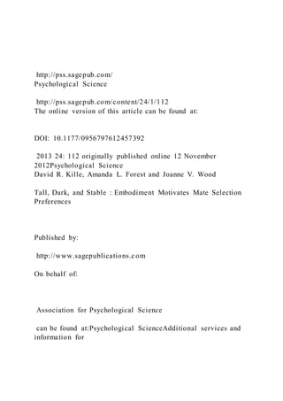
A one-way analysis of variance (ANOVA) revealed that, as
predicted, participants in the physically unstable condition
perceived less stability in other people’s relationships (M =
4.80, SD = 1.12) than did participants in the physically stable
condition (M = 5.55, SD = 0.84), F(1, 43) = 6.28, p = .016,
ηp
2 = .13 (Fig. 1). These results suggest that physical instabil-
ity activates the concept of instability more broadly.
More important, physical instability affected preferences:
7. A one-way ANOVA revealed that participants in the physi-
cally unstable condition reported a greater desire for stability
traits in a partner (M = 5.00, SD = 0.78) than did participants
in the physically stable condition (M = 4.38, SD = 0.72), F(1,
45) = 8.18, p = .006, ηp
2 = .15 (see Fig. 1). No differences
between conditions emerged in preference for stability-neutral
traits, F < 1, or in mood, except that participants in the physi -
cally unstable condition felt happier than participants in the
physically stable condition, F(1, 40) = 4.44, p = .041, ηp
2 =
.10. Two analyses regressing preferences and perceptions onto
happiness and condition indicated that happiness was unre-
lated to either outcome (ts < 1).
Discussion
Our study confirms that subtle bodily experiences affect not
only people’s perceptions of others, but also their preferences in
others: Participants who experienced physical instability per -
ceived less stability in other people’s relationships and desired
more stability in their own potential partners than did partici -
pants who did not experience such instability. Moreover, pilot
testing suggested that participants in the physically unstable
condition did not simply prefer more positive traits; using a
Likert-type scale (1 = relatively negative/undesirable/not very
fun, 9 = relatively positive/desirable/very fun), 24 participants
rated the traits in the stability composite as being marginally
less positive (M = 7.19, SD = 0.94) than the traits in the
stability-
neutral composite (M = 7.44, SD = 0.81), t(23) = 1.89, p = .071.
Consequently, we concluded that physical instability altered
participants’ motivation to seek psychological stability rather
than their motivation to seek positively valenced traits.
8. Mate selection is often viewed as a process that reflects
long-term goals rather than in-the-moment psychological
needs. The present study suggests that mate preferences may
shift with transient bodily states created by the physical envi -
ronment. By examining the important outcome of preferences
in mate selection (Meier et al., 2012), this study extends previ -
ous findings suggesting that the physical world can affect pref-
erences for movie genres (Hong & Sun, 2012) and cleansing
products (Zhong & Liljenquist, 2006). We suspect that previ -
ously studied physical states may also motivate mate selec-
tion: For example, given that physical dirtiness is linked to
moral impurity (see Lee & Schwarz, 2011), examining dating
profiles in a physically dirty environment might motivate peo-
ple to seek out moral puritans. Additionally, because perceived
power is associated with feeling tall (Duguid & Goncalo,
2012), feeling short—as when seated in a lowered chair—
could increase the attractiveness of high-status mates.
Our results also suggest that embodied cues can affect
motivation, because participants’ preferences (for stability)
likely reflected their goals (to achieve stability). Insofar as
goals and motivational states are represented as cognitive
structures (Kruglanski et al., 2002), those structures should be
represented—much like any other cognition—through senso-
rimotor information (Barsalou, 2008). Indeed, we suspect that
one reason cognition may become embodied is to ensure that
one’s needs—which may arise from physical states—are met
through goal pursuit. Embodied motivation, then, is a fruitful
avenue for future research.
Acknowledgments
The authors thank Vanessa K. Bohns, Richard P. Eibach, and
John G.
Holmes for their invaluable comments on an earlier draft, and
Alix
9. Collins and Lindsay Stehouwer for their assistance in
conducting this
research.
3.00
3.50
4.00
4.50
5.00
5.50
6.00
6.50
7.00
Perceptions of Stability Preference for Stability
R
at
in
g
Physically Stable Condition
Physically Unstable Condition
Fig. 1. Mean perception of other people’s relationship stability
and
10. mean preference for stability (vs. instability) traits in a
potential mate as
a function of physical stability condition. Error bars represent
standard
errors of the mean.
at OhioLink on February 14, 2013pss.sagepub.comDownloaded
from
http://pss.sagepub.com/
114 Kille et al.
Declaration of Conflicting Interests
The authors declared that they had no conflicts of interest with
respect to their authorship or the publication of this article.
Funding
This research was supported by a Social Sciences and
Humanities
Research Council of Canada grant awarded to Joanne V. Wood.
References
Ainsworth, M. D. S. (1979). Infant-mother attachment.
American
Psychologist, 10, 932–937.
Barsalou, L. W. (2008). Grounded cognition. Annual Review of
Psy-
chology, 59, 617–645.
Bowlby, J. (1988). A secure base: Parent-child attachment and
healthy human development. New York, NY: Basic Books.
11. Chappell, K. D., & Davis, K. E. (1998). Attachment, partner
choice,
and perception of romantic partners: An experimental test of the
attachment-security hypothesis. Personal Relationships, 3, 117–
136.
Collins, N. L., & Feeney, B. C. (2000). A safe haven: Support-
seeking and caregiving processes in intimate relationships.
Jour-
nal of Personality and Social Psychology, 78, 1053–1073.
Duguid, M. M., & Goncalo, J. A. (2012). Living large: The
powerful
overestimate their own height. Psychological Science, 23, 36–
40.
Higgins, E. T. (2012). Beyond pleasure and pain: How
motivation
works. New York, NY: Oxford University Press.
Hong, J., & Sun, Y. (2012). Warm it up with love: The effect of
physi-
cal coldness on liking of romance movies. Journal of Consumer
Research, 39, 293–306.
Kruglanski, A. W., Shah, J. Y., Fishbach, A., Friedman, R.,
Chun,
W. Y., & Sleeth-Keppler, D. (2002). A theory of goal systems.
In
M. P. Zanna (Ed.), Advances in experimental social psychology
(Vol. 34, pp. 331–378). San Diego, CA: Academic Press.
Lee, S. W. S., & Schwarz, N. (2011). Wiping the slate clean:
Psycho-
logical consequences of physical cleansing. Current Directions
in
12. Psychological Science, 20, 307–311.
Meier, B. P., Schnall, S., Schwarz, N., & Bargh, J. A. (2012).
Embodi-
ment in social psychology. Topics in Cognitive Science, 4, 705–
716. doi: 10.1111/j.1756-8765.2012.01212.x
Williams, L. E., & Bargh, J. A. (2008). Experiencing physical
warmth
influences interpersonal warmth. Science, 322, 606–607.
Zhong, C.-B., & Liljenquist, K. (2006). Washing away your
sins:
Threatened morality and physical cleansing. Science, 313,
1451–
1452.
at OhioLink on February 14, 2013pss.sagepub.comDownloaded
from
http://pss.sagepub.com/
moving averageFile name: best homesUse this worksheet to
analyze the best homes case study.The data is entered into 60
rows. One row for each month.The forecasting model can be
entered into the columns.1Jan 118402Feb 118803Mar
1111204Apr 1112005May 1111206Jun
111120122001016.77July 111080122801023.38Aug
111000126001050.09Sept 11960128401070.010Oct
111000130001083.311Nov 11920132801106.712Dec
11960135201126.713Jan 12920137601146.714Feb
121200140001166.715Mar 121360142401186.716Apr
121360144001200.017May 121400146001216.718Jun
121360147601230.019July 121320151201260.020Aug
121240153601280.021Sept 121200156401303.322Oct
121160160001333.323Nov 121120162001350.024Dec
27. data.
Questions for the case
1. What forecasting methods should the company consider?
Please justify.
2. Use the classical decomposition method to forecast average
demand for 2016 by month. What is your forecast of monthly
average demand for 2016?
3. Best Homes is also collecting sales projections from each of
its regions for 2016? What role should these additional sales
projections play, along with the forecast from question 2 in
determining the final national forecast?
I hope this helps
If not we can have an adobe session with your team tomorrow
Sunday April 12, 2020 or any other time that is convenient
Regards,
Santosh Sambare
Best Homes, Inc.: Forecasting
28. Background
Best Homes is a new home construction company based in
Kansas City, Missouri. They build only residential and new
homes throughout the United States. They have expanded the
Midwest and the West coast and to the south, starting in 1945
the East coast. They build all types of new residential housing,
from low-end to high-end housing in the market. Best Homes
was a private company until 1958 when the initial public
offering began. The company started small but expanded to one
of the largest home builders in the United States. The case
presents monthly sales data from 2011 to 2015. This data is
representative of home builders since we estimated the sales of
Best Homes based on a 4% market share of the total sales of
new homes in the U.S. from the U.S. Census web site. Thus,
the trend and seasonality are in line with U.S. home sales in
total. The case explains the problem facing Best Homes in terms
of annual planning and the S&OP process. Forecasting is put in
the context of how the forecast will be used. Also, sales
projections are being gathered from the field, and the case asks
students to reconcile those with the forecasts based on historical
data. Best Homes competes on the basis of their outstanding
brand reputation. Their reputation is gained by building quality
houses at competitive prices. The cost per square foot of the
house is comparable to that of its competitors, but its design
and interior finish are excellent. This provides an advantage
that competitors can't find. Show after completion of the
building, including the installation of inner walls, floors,
windows, siding, cabinets and timber works, to provide a
beautiful home. Use part-time or contract for other parts that are
not marked upon completion. However, workers who perform
foundations, rough walls, roofs, wiring and piping. In each of
these areas, however, they employ more than 60 percent of ful l-
time workers. All new employees, part-time or contract
employees are assigned full-time employees and receive quality
control training for their work during the first six months.
29. Objective
Financing uses this to forecast the company's overall revenue
and to prepare estimates of revenue and balance sheet forecasts
along with quarterly income estimates. Marketing uses monthly
forecasts to plan sales forecasts, employment plans, sales
incentives and sales targets. Operations and supply chains use
forecasts for sales and operational planning (S & OP) planning
processes. S & OP is performed for annual forecasts and
updated monthly to coordinate sales forecasts and resulting
employment plans for new, contracted and part-time employees.
Along with the expected dismissal. Each month, the S & OP
process starts with an updated rolling forecast every 12 months.
The employment plan and the start of housing construction are
then set up next month and planned for the next three months.
The plan also includes a purchase plan for materials used in
construction. Housing. Monthly updates may require adjusting
both the capacity and inventory of new homes. All features,
including finance, marketing, sales, operations, and HR,
participate in the S & OP process. The first part of the planning
process is to predict the demand for new homes every month.
Shows the number of detached houses built by Best Homes
every month. This data is a forward forecast for all of 2016.
Predicting average monthly demand alone in the future is not
enough. Actual demand may be significantly higher or lower
than average. As a result, you should also predict standard or
average absolute deviations. The monthly production level of
the new house is set to average demand. In addition, if demand
exceeds the average, secure a safe inventory of new homes.
With three months of lead time to build a new house, all
inventory and production levels should expect three months of
lead time. This shows an important prediction for both
30. predictions.
1. What forecasting methods should the company consider?
Please justify.
· The company should use time series method
· It suitable for not much data and based on seasonal patterns
· According to the calculation the 12 months moving average.
· The advantages of this method are easy to understand, and the
moving average can smooth the estimate that makes the
company see the trend.
· The moving average can be calculated by using the previous
sale and calculate the average.
1
Jan 11
840
2
Feb 11
880
3
Mar 11
1120
4
Apr 11
1200
5
May 11
1120
40. 71
Nov 16
72
Dec 16
2. Use the classical decomposition method to forecast average
demand for 2016 by month. What is your forecast of monthly
average demand for 2016?
· As a result, the blue trend is a sale forecast and the orange
trend is calculated sale with the 12 months moving average
· The linear function from the sale itself is y = 11.758x+1003.4
where r-square is 0.5888
· The linear function from 12 months moving average is
12.442x+925.28 where r-square is 0.9504
· R-square can describe How accurate of the function which has
value between 0-100%
41. · When we compare the 12 months average r-square with the
sale r-square the 12 months average r-square is more accurate
· The company should use 12 months moving average function
y=12.442x+925.28 where x is a month order start from January
2011 to forecast monthly average demand for 2016
X
Month
MOV AVG FCT
61
Jan 16
1684.4
62
Feb 16
1696.8
63
Mar 16
1709.2
64
Apr 16
1721.7
65
May 16
1734.1
42. 66
Jun 16
1746.6
67
July 16
1759.0
68
Aug 16
1771.5
69
Sept 16
1783.9
70
Oct 16
1796.3
71
Nov 16
1808.8
72
Dec 16
1821.2
3. Best Homes is also collecting sales projections from each
of its regions for 2016? What role should these additional sales
projections play, along with the forecast from question 2 in
determining the final national forecast?
Year
2011
2012
2013
2014
2015
2016
Moving average total
12075
43. 13867
15659
17450
19242
21034
Growth rate
15%
13%
11%
10%
9%
· The sale growth rate has dropped since 2012. If the company
focus only number of sales which is growth overtime will start
to lose market competitive.
· This comparison of growth rate will lead to discussion of
developing the company’s marketing, operation, finance, and
human resource.
· However, the sale projection from all region will help
assuming the overall demand forecast it help to manage the
reasonable inventory which can prevent over operation cost and
inventory cost.
Moving Average 12 Preceding Months
SALES
1 2 3 4 5 6 7 8 9 10 11 12 13
14 15 16 17 18 19 20 21 22 23 24 25
26 27 28 29 30 31 32 33 34 35 36 37
38 39 40 41 42 43 44 45 46 47 48 49
50 51 52 53 54 55 56 57 58 59 60