![References
S. D. Chowdhury, J. R. David and Shiroman Prakash, “Spectral sum rules for
conformal field theories in arbitrary dimensions”, JHEP07(2017)119.
S. D. Chowdhury, J. R. David and S. Prakash, “Constraints on parity violating
conformal field theories in d = 3”, [arXiv:1707.03007[hep-th]].
Ongoing Work.
Subham Dutta Chowdhury Conformal field theories and three point functions 2/51](https://image.slidesharecdn.com/uchicago-171113135150/75/Conformal-field-theories-and-three-point-functions-2-2048.jpg)
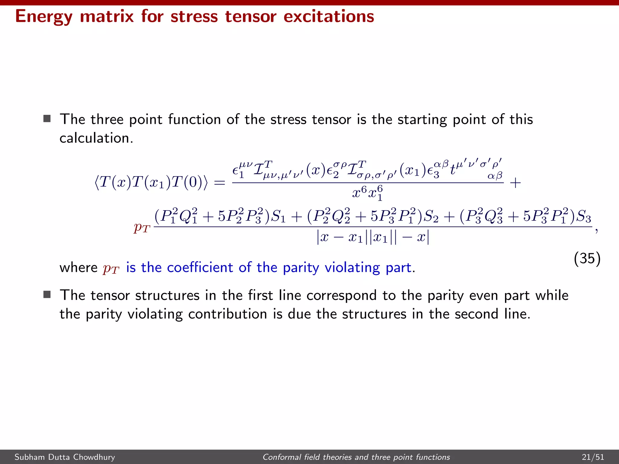
![Consider a conformal field theory with a conserved stress tensor T in d = 4.
Conformal invariance restricts the structure of the three point functions of T,
to be of the following form,
TTT = nT
s TTT free boson + nT
f TTT free fermion + nT
v TTT vector,
where .. free boson, .. free fermion denote the correlator a real free boson and a
real free fermion respectively, while .. vector refers to the vector boson.
[Osborn, Petkou 1994]
The numerical coefficients nT
s , nT
f and nT
v correspond to effective number of
scalars, fermions and vector bosons respectively.
Note that in higher dimensions, nT
v corresponds to correlation functions of
k-forms and is non zero only for even dimensions.
Subham Dutta Chowdhury Conformal field theories and three point functions 4/51](https://image.slidesharecdn.com/uchicago-171113135150/75/Conformal-field-theories-and-three-point-functions-4-2048.jpg)
![For parity even conformal field theories in d = 4 and higher dimensions,
conformal collider bounds impose constraints on the parity even coefficients
that occur in the three point functions.
[Maldacena, Hofman 2008]
[De Boer et al , Sinha et al. 2009]
This involves studying the effect of localized perturbations at the origin. The
integrated energy flux per unit angle, over the states created by such
perturbations, is measured at a large sphere of radius r.
Eˆn =
0|O†
EˆnO|0
0|O†O|0
,
Eˆn = lim
r→∞
r2
∞
−∞
dtni
Tt
i (t, rˆn),
O ∼
ij
Tij
ijTij|Tij
ij
,
i
ji
jjj|ji
i
,
(1)
where, ˆn is a unit vector in R3
, which specifies the direction of the calorimeter
and O is the operator creating the localised perturbation.
Subham Dutta Chowdhury Conformal field theories and three point functions 5/51](https://image.slidesharecdn.com/uchicago-171113135150/75/Conformal-field-theories-and-three-point-functions-5-2048.jpg)
![For parity invariant theories in general dimensions, causality constraints in
terms of these variables is given by
[Camanho, Edelstein 2009]
1 −
1
d − 1
t2 −
2
(d + 1)(d − 1)
t4 ≥ 0, (5)
1 −
1
d − 1
t2 −
2
(d + 1)(d − 1)
t4 +
1
2
t2 ≥ 0,
1 −
1
d − 1
t2 −
2
(d + 1)(d − 1)
t4 +
d − 2
d − 1
(t2 + t4) ≥ 0.
Can such constraints be used to put bounds on physical quantities of CFTs at
finite temperature?
Moreover, physically relevant examples of confromal field theories, in d = 3,
need not preserve parity owing to the presence of a parity violating chern
simons term.
Subham Dutta Chowdhury Conformal field theories and three point functions 7/51](https://image.slidesharecdn.com/uchicago-171113135150/75/Conformal-field-theories-and-three-point-functions-7-2048.jpg)
![Let us consider a conformal field theory in d = 3 with a U(1) conserved current
j and conserved stress tensor T and let the theory be parity violating.
Conformal invariance restricts the structure of the three point functions of j
and T, in d = 3, to be of the following form,
jjT = nj
s jjT free boson + nj
f jjT free fermion + pj jjT parity odd, (6)
TTT = nT
s TTT free boson + nT
f TTT free fermion + pT TTT parity odd,
where, as before, .. free boson, .. free fermion denote the correlator a real free
boson and a real free fermion respectively, while .. parity odd refers to the
parity odd structure.
[Osborn, Petkou 1994]
[Giombi, Prakash, Yin 2011]
The numerical coefficients nj,T
s , nj,T
f correspond to the parity invariant sector,
while pj,T is the parity violating coefficient. The parity violating structure is
unique to d = 3 and it appears only for interacting theories.
Subham Dutta Chowdhury Conformal field theories and three point functions 8/51](https://image.slidesharecdn.com/uchicago-171113135150/75/Conformal-field-theories-and-three-point-functions-8-2048.jpg)
![Positivity of energy flux
Let us consider localised perturbations of the CFT in minkowski space.
ds2
= −dt2
+ dx2
+ dy2
. (9)
The perturbations evolve and spread out in time. In order to measure the flux,
we consider concentric circles.
The energy measured in a direction (denoted by ˆn) is defined by,
Eˆn = lim
r→∞
r
∞
−∞
dt ni
Tt
i (t, rˆn), (10)
where r is the radius of the circle on which the detector is placed and ˆn is a unit
vector which determines the point on the circle where the detector is placed.
The expectation value of the energy flux measured in such a way should be
positive for any state.
[Maldacena, Hofman 2008]
Eˆn ≥ 0. (11)
Subham Dutta Chowdhury Conformal field theories and three point functions 10/51](https://image.slidesharecdn.com/uchicago-171113135150/75/Conformal-field-theories-and-three-point-functions-10-2048.jpg)
![We can also consider the detector to be placed at null infinity from the very
beginning and integrate over the null working time. The two definitions are
equivalent.
[Zhiboedov 2013]
In order to calculate energy flux at null infinity, we introduce the light cone
coordinates, x±
= t ± y. We place our detector along y direction. The energy
functional becomes
E =
∞
−∞
dx−
2
lim
x+→∞
(
x+
− x−
2
)T−−. (12)
We are interested in expectation value of the energy operator on states created
by stress tensor or current with specific polarizations.
Subham Dutta Chowdhury Conformal field theories and three point functions 11/51](https://image.slidesharecdn.com/uchicago-171113135150/75/Conformal-field-theories-and-three-point-functions-11-2048.jpg)
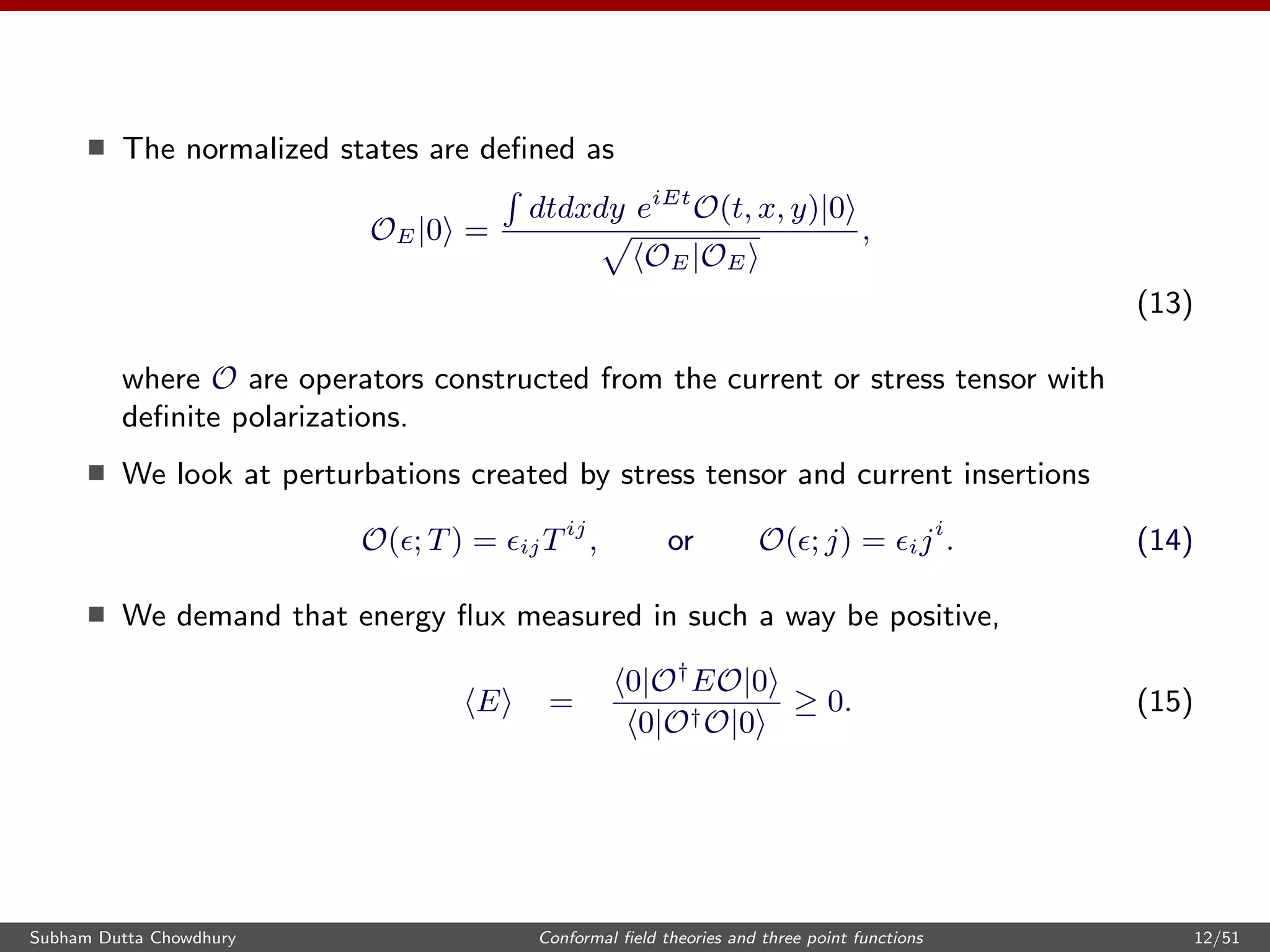
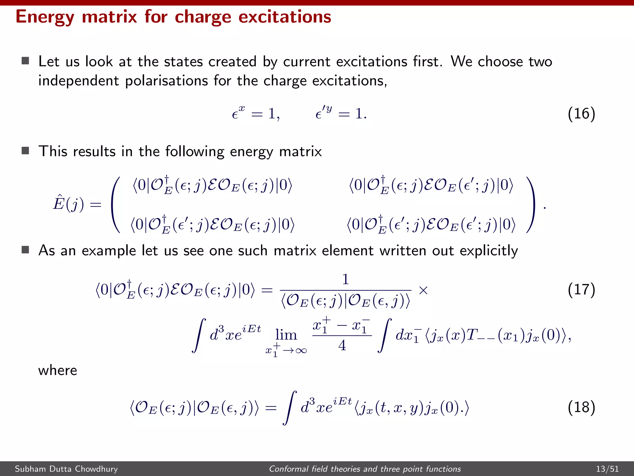
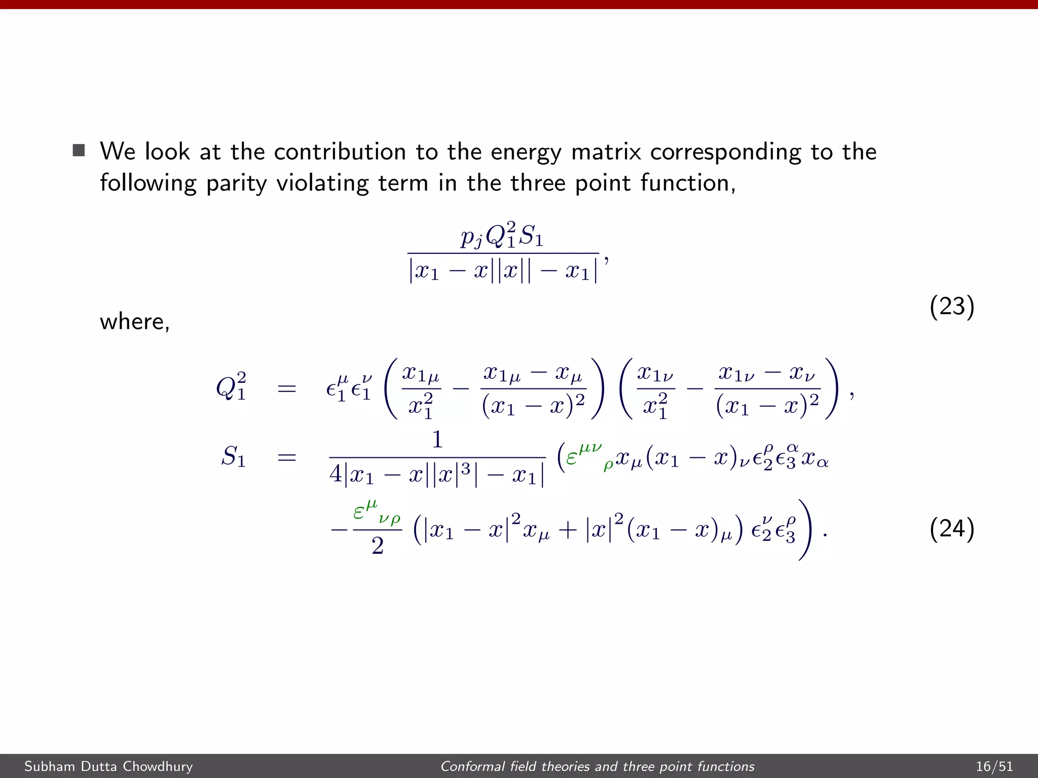
![The condition of positivity of energy functional measured by the calorimeter
then translates to demanding that the eigenvalues of the energy matrix be
positive.
The basic ingredient in this computation is the three point function of the
stress energy tensor including the parity odd term.
j(x)T(x1)j(0) =
1
|x1 − x|3|x1|3|x|
σ
2 Iα
σ (x − x1) ρ
3Iβ
ρ (−x1) µν
1 tµναβ(X)
+pj
Q2
1S1 + 2P2
2 S3 + 2P2
3 S2
|x1 − x||x|| − x1|
, (19)
where pj is the parity odd coefficient.
[Osborn, Petkou 1994]
[Giombi, Prakash, Yin 2011]
The first line corresponds to the usual parity even contribution while the 2nd
part is the parity odd contribution to the three point function.
Subham Dutta Chowdhury Conformal field theories and three point functions 14/51](https://image.slidesharecdn.com/uchicago-171113135150/75/Conformal-field-theories-and-three-point-functions-14-2048.jpg)
![Large N Chern Simons theories
U(N) Chern Simons theory at level κ coupled to either fermions or bosons in
the fundamental representation are examples of conformal field theories which
violate parity. In the large N limit, these can be solved to all orders in the ’t
Hooft coupling
[Giombi et al, 2011]
[Aharony et al, 2011]
We consider U(N) Chern Simons theory at level κ coupled to fundamental
fermions.
The coefficients for the three point functions at the large N limit (planar limit)
are given by,
nT
s (f) = nj
s(f) = 2N
sin θ
θ
sin2 θ
2
, nT
f (f) = nj
f (f) = 2N
sin θ
θ
cos2 θ
2
,
pj(f) = α N
sin2
θ
θ
, pT (f) = αN
sin2
θ
θ
,
where the t ’Hooft coupling is related to θ by
θ =
πN
κ
. (39)
[Maldacena, Zhiboedov 2012]
Subham Dutta Chowdhury Conformal field theories and three point functions 23/51](https://image.slidesharecdn.com/uchicago-171113135150/75/Conformal-field-theories-and-three-point-functions-23-2048.jpg)
![The numerical coefficients α, α can be determined by a one loop computation
in the theory with fundamental fermions.
[Giombi et al, 2011]
We repeat the analysis to precisely determine the factors α, α .
α =
3
π4
, α =
1
π4
. (40)
The parameters of the three point function take the form
a2 = −2 cos θ, αj = 2 sin θ, t4 = −4 cos θ, αT = 4 sin θ. (41)
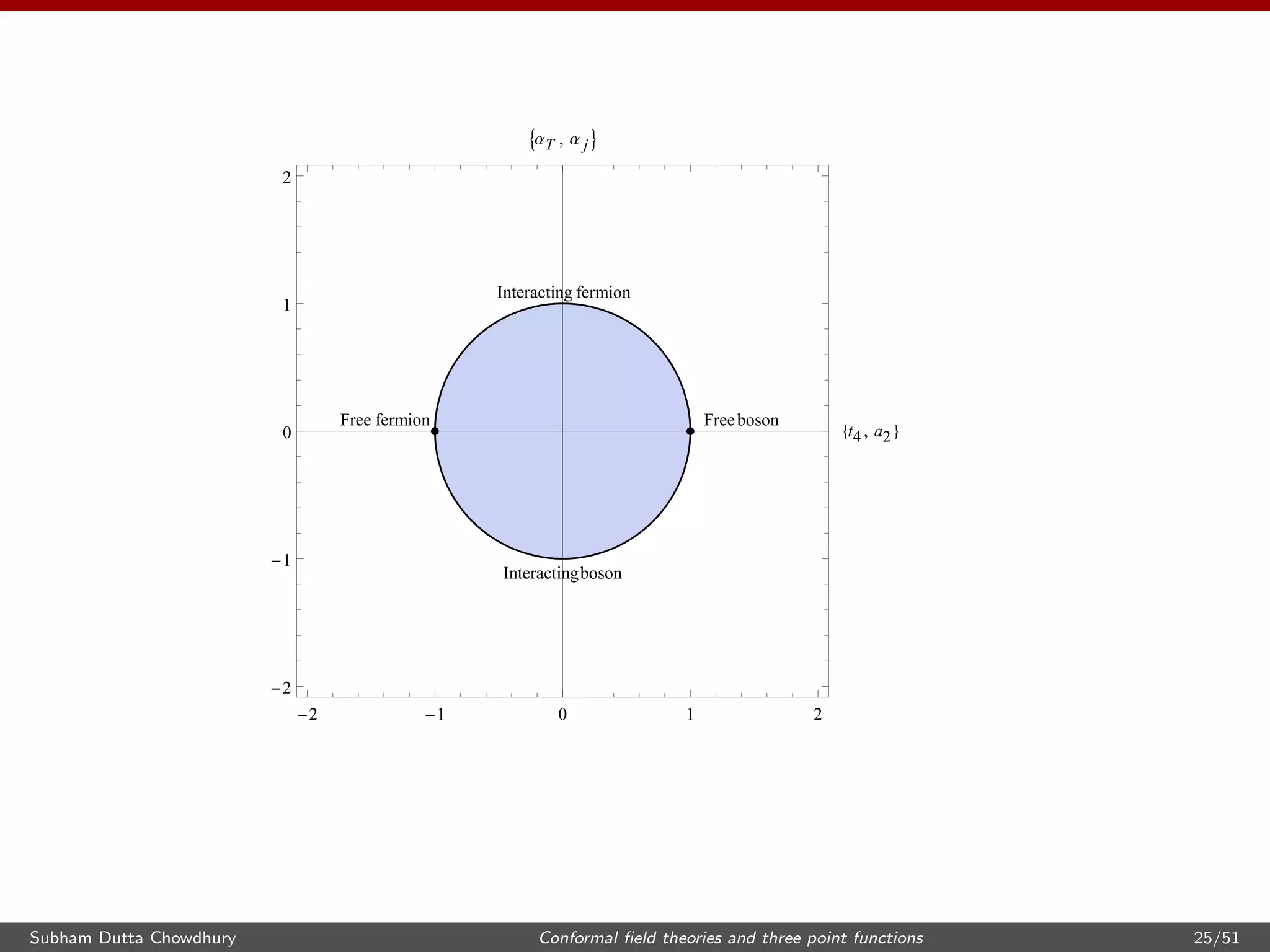
Thus the Chern-Simons theories with a single fundamental boson or fermion
saturate the conformal collider bounds and they lie on the circles
a2
2 + α2
j = 4, t2
4 + α2
T = 16. (42)
The location of the theory on the circle is given by θ the t ’Hooft coupling.
Subham Dutta Chowdhury Conformal field theories and three point functions 24/51](https://image.slidesharecdn.com/uchicago-171113135150/75/Conformal-field-theories-and-three-point-functions-24-2048.jpg)
![We aim to compute sum rules for conformal field theories in d > 2. An
operator universal to CFTs is the stress tensor Tµν . We will look at the sum
rule for the retarded correlator,
GR(t, x) = iθ(t) [Txy(t, x), Txy(0)] .
(44)
at finite temperature and zero chemical potential
We assume that no other operators apart from the stress tensor gets
expectation values.
The Fourier transform of the retarded correlator is given by,
GR(ω, 0) = dd
xeiωt
GR(t, x) (45)
Subham Dutta Chowdhury Conformal field theories and three point functions 27/51](https://image.slidesharecdn.com/uchicago-171113135150/75/Conformal-field-theories-and-three-point-functions-27-2048.jpg)
![At high frequencies the retarded correlator exhibits a divergent behaviour.
In order to understand this behavior in a precise manner, we analytically
continue GR(ω) into the upper half plane
GR(i2πnT) = GE(2πnT). (50)
Here GE is the Euclidean time ordered correlator and 2πnT is the Matsubara
frequency.
Consider the Euclidean correlator in position space. For time intervals
δt β = 1
T
, the operator product expansion (OPE) of the stress tensor offer a
good asymptotic expansion. Therefore for ω T, we can replace the
Euclidean correlator by its OPE. This allows us to obtain the asymptotic
behaviour of the GR(iω) as ω → ∞.
[Romatschke, Son, 2009]
Subham Dutta Chowdhury Conformal field theories and three point functions 30/51](https://image.slidesharecdn.com/uchicago-171113135150/75/Conformal-field-theories-and-three-point-functions-30-2048.jpg)
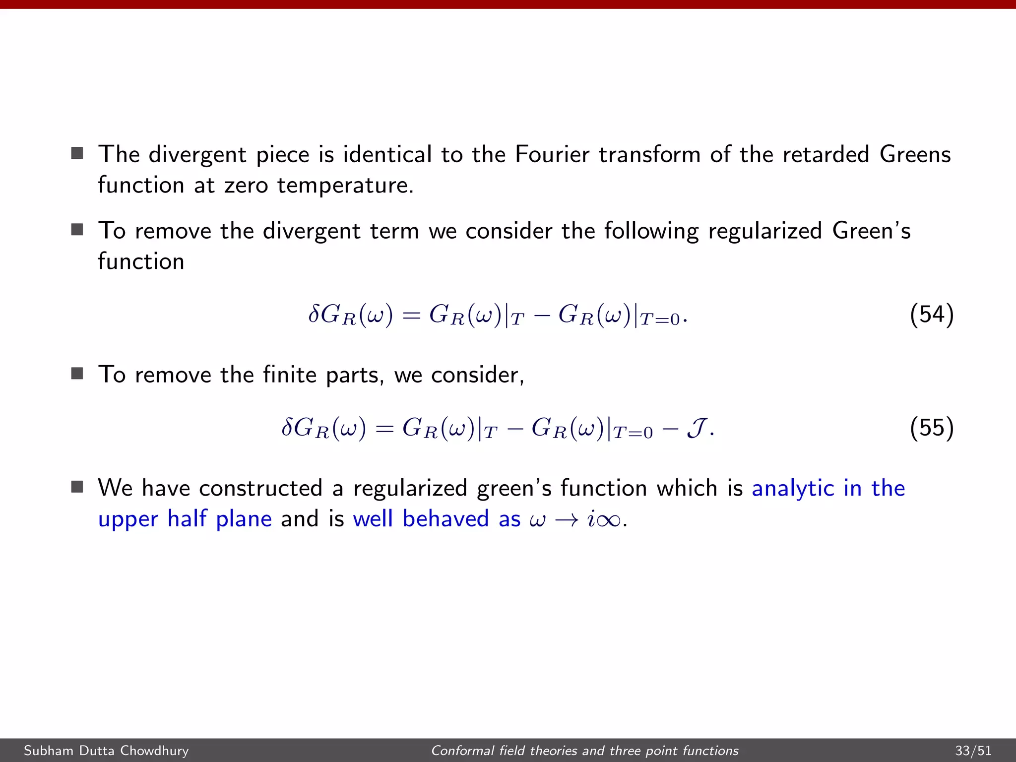
![The sum rule then becomes,
lim
→0+
1
π
∞
−∞
δρ(ω)dω
ω − i
= δGR(0),
GR(t, x) = iθ(t)[Txy(t, x), Txy(0)],
(56)
where δρ(ω) is the difference of spectral densities
δρ(ω) = Im(GR(0)|T − GR(0)|T =0)
= ρ(ω) − ρ(ω)T =0,
δGR(0) = GR(0)|T − GR(0)|T =0 − J . (57)
Note that the finite term does not feature in the difference of spectral densities.
It will turn out to be real and will not contribute to the spectral densities.
The first term is obtained from the hydrodynamic behaviour of the theory while
high frequency behaviour is captured by the OPE.
Subham Dutta Chowdhury Conformal field theories and three point functions 34/51](https://image.slidesharecdn.com/uchicago-171113135150/75/Conformal-field-theories-and-three-point-functions-34-2048.jpg)
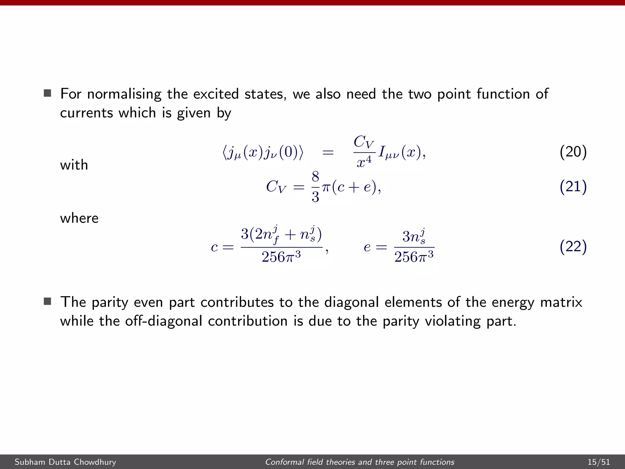
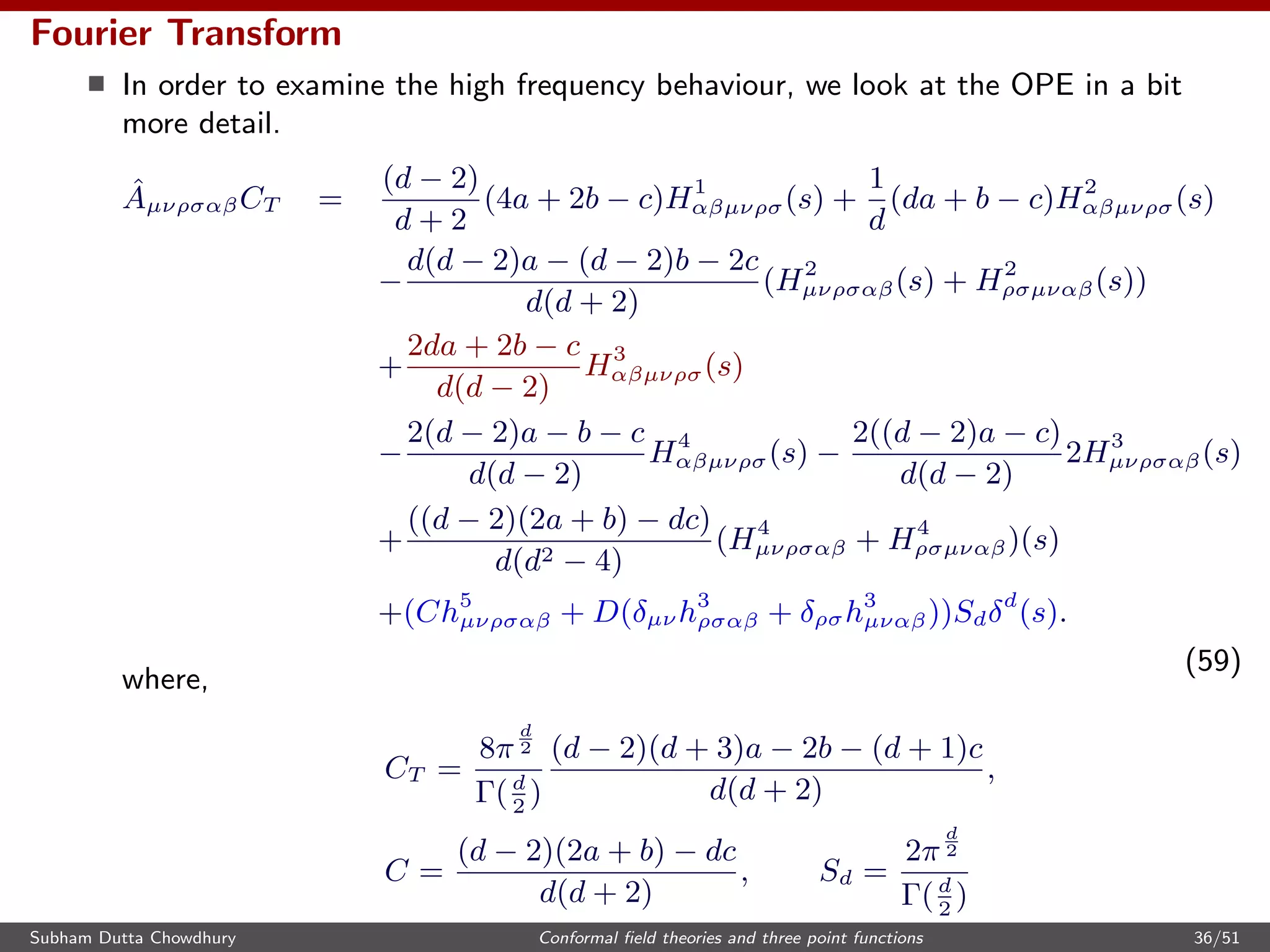
![Shear sum rule d ≥ 3
The OPE of the Euclidean two point function in general dimensions is well
studied.
The tensor structures in OPE are as follows,
Txy(s)Txy(0) ∼ CT
Ixy,xy(s)
s2d
+ ˆAxyxyαβ(s) Tαβ(0) + · · · (58)
[Osborn, Petkou 1993]
where CT is the normalization of the two point function of the stress tensor.
The coefficients are determined in terms of the parameters of the three point
function of the stress tensor (a, b, c)
Note that for d = 3, there is no additional contribution from the parity odd
structure, for the shear channel.
Subham Dutta Chowdhury Conformal field theories and three point functions 35/51](https://image.slidesharecdn.com/uchicago-171113135150/75/Conformal-field-theories-and-three-point-functions-35-2048.jpg)
![We fourier transform all the terms in the OPE and we obtain,
J = A + B
A =
(1 − d)P(a(d(d + 4) − 4) + d(2b − c))
2 (−a (d2 + d − 6) + 2b + cd + c)
B =
((2a + b)(−2 + d) − cd)P
−2b − c(1 + d) + a (−6 + d + d2)
,
(60)
A is the contribution from tensor structures and B is the contribution from the
contact term.
The contribution A, due the tensor structures without the contact terms, is
proportional to the Hofman-Maldacena coefficient in general d dimensions.
[Meyers, Sinha 2009]
Subham Dutta Chowdhury Conformal field theories and three point functions 37/51](https://image.slidesharecdn.com/uchicago-171113135150/75/Conformal-field-theories-and-three-point-functions-37-2048.jpg)
![Holography Check 1
The coefficients a, b, c have been evaluated in AdSd+1 by evaluating the 3
point function of the stress tensor holographically.
[Arutyunov, Frolov 1999]
a = −
d4
π−d
Γ[d]
4(−1 + d)3
,
b = −
d 1 + (−3 + d)d2
π−d
Γ(1 + d)
4(−1 + d)3
,
c =
d3
(1 − 2(−1 + d)d)π−d
Γ(d)
4(−1 + d)3
.
(64)
Evaluating A and B, we have,
A = −
d
2(d + 1)
, B = P (65)
Subham Dutta Chowdhury Conformal field theories and three point functions 39/51](https://image.slidesharecdn.com/uchicago-171113135150/75/Conformal-field-theories-and-three-point-functions-39-2048.jpg)
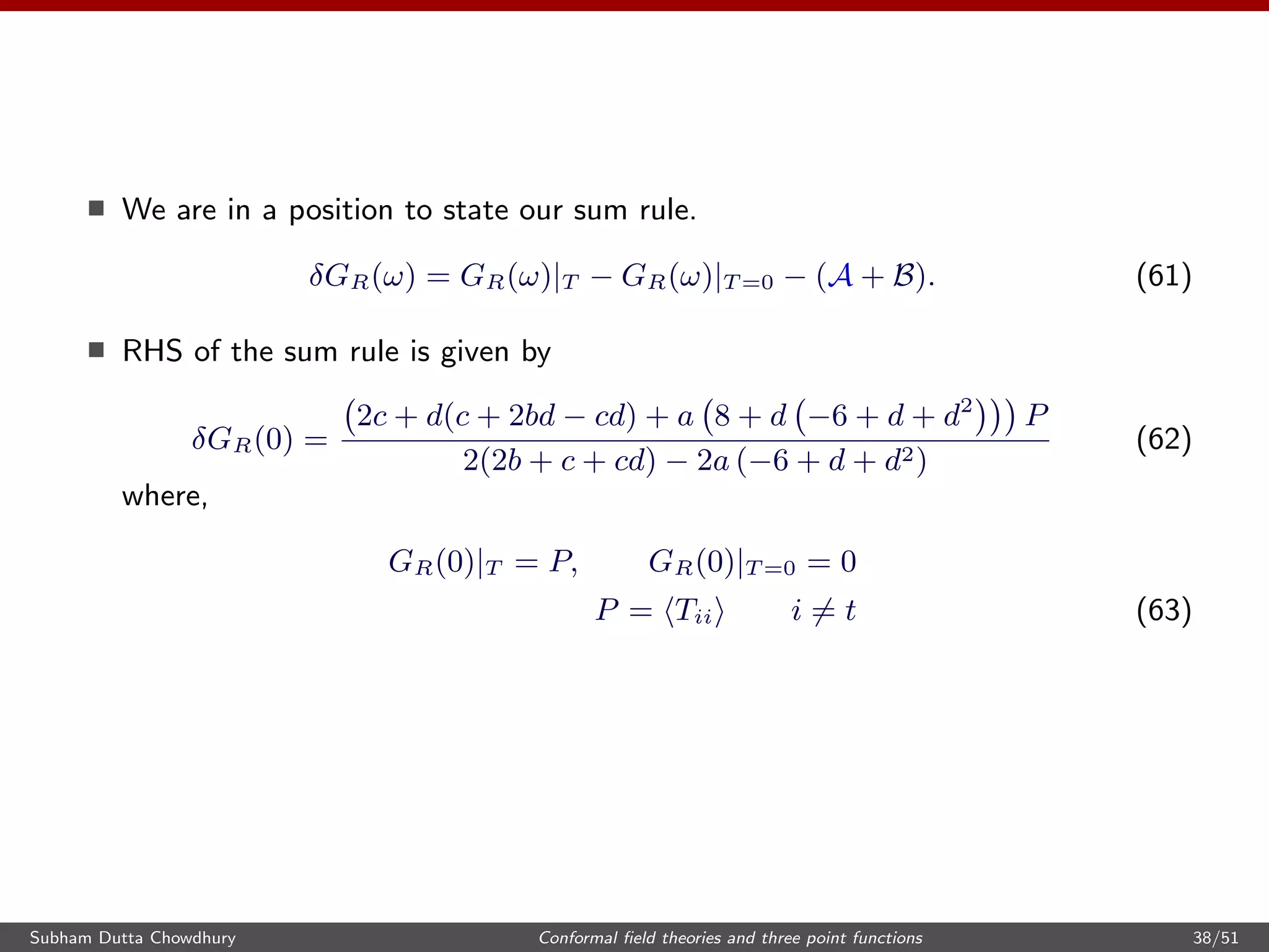
![We now evaluate the sum rule,
δGR(0) =
d
2(d + 1)
lim
→0+
1
π
∞
−∞
δρ(ω)dω
ω − i
=
d
2(d + 1)
(66)
For d = 4 this becomes
lim
→0+
1
π
∞
−∞
δρ(ω)dω
ω − i
=
2
5
(67)
[Son, Romatschke 2009]
Subham Dutta Chowdhury Conformal field theories and three point functions 40/51](https://image.slidesharecdn.com/uchicago-171113135150/75/Conformal-field-theories-and-three-point-functions-40-2048.jpg)
![Holography Check 2
An alternate way of deriving the sum rule is to directly study the Green’s
functions in AdSd+1 black hole background and obtain the high frequency
behaviour.
The shear sum rule was first studied holographically in the context of AdS5.
[Son, Romatschke 2009]
This method of directly evaluating green’s function was generalised to arbitrary
dimensions by Herzog et al. The analyticity of the Green’s functions in the
upper half plane is obtained by studying the differential equations.
[Gulotta, Herzog, Kaminski 2010]
Modifications to the shear sum rule for retarded correlators of stress tensor as
well as currents in presence of chemical potential have also been studied.
[Jain, Thakur, David 2011],
[Thakur, David 2012],
Subham Dutta Chowdhury Conformal field theories and three point functions 41/51](https://image.slidesharecdn.com/uchicago-171113135150/75/Conformal-field-theories-and-three-point-functions-41-2048.jpg)
![Using Cauchy’s theorem then one gets for general dimensions,
1
π
∞
−∞
dω
ω
[ρ(ω) − ρT =0(ω)] =
d
2(d + 1)
(68)
This is a consistency check for shear sum rule of conformal field theories in
arbitrary dimensions.
[Gulotta, Herzog, Kaminski 2010]
From this we come to the conclusion that, the parameters of the three point
function of stress tensor of any conformal field theory with a two derivative
gravity dual must satisfy the following constraint.
2c + d(c + 2bd − cd) + a 8 + d −6 + d + d2
2(2b + c + cd) − 2a (−6 + d + d2)
=
d(d − 1)
2(d + 1)
(69)
Subham Dutta Chowdhury Conformal field theories and three point functions 42/51](https://image.slidesharecdn.com/uchicago-171113135150/75/Conformal-field-theories-and-three-point-functions-42-2048.jpg)
![Applications in d = 4
Positivity of energy flux/ Causality constraints lead to certain bounds on the
parameters of the three point function of the stress tensor.
[Hofman, Maldacena 2008]
−
t2
3
−
2t4
15
+ 1 ≥ 0
2 −
t2
3
−
2t4
15
+ 1 + t2 ≥ 0
3
2
−
t2
3
−
2t4
15
+ 1 + t2 + t4 ≥ 0 (70)
We can rewrite the general sum rule for d = 4 in terms of collider variables to
get
δGR(0) = (
6
5
−
t2
6
−
2t4
75
)P (71)
The causality bounds then translate to the following bounds on the sum rule
P
2
≤ δGR(0) ≤ 2P (72)
The lower bound is saturated for theories with only free fermions, while the
upper bound is saturated for theories with only free bosons.
Subham Dutta Chowdhury Conformal field theories and three point functions 43/51](https://image.slidesharecdn.com/uchicago-171113135150/75/Conformal-field-theories-and-three-point-functions-43-2048.jpg)
![There is a similar parametrization of the parameters of the three point
functions, in d dimensions, in terms of t2, t4.
[Buchel et al 2009]
The general expression for sum rule can be expressed in terms of these
parameters.
δGR(0) =
(−1 + d)d
2(1 + d)
+
(3 − d)t2
2(−1 + d)
+
2 + 3d − d2
t4
(−1 + d)(1 + d)2
P (73)
The Causality constraints in terms of these variables is given by
[Camanho, Edelstein 2009]
1 −
1
d − 1
t2 −
2
(d + 1)(d − 1)
t4 ≥ 0, (74)
1 −
1
d − 1
t2 −
2
(d + 1)(d − 1)
t4 +
1
2
t2 ≥ 0,
1 −
1
d − 1
t2 −
2
(d + 1)(d − 1)
t4 +
d − 2
d − 1
(t2 + t4) ≥ 0.
Subham Dutta Chowdhury Conformal field theories and three point functions 44/51](https://image.slidesharecdn.com/uchicago-171113135150/75/Conformal-field-theories-and-three-point-functions-44-2048.jpg)
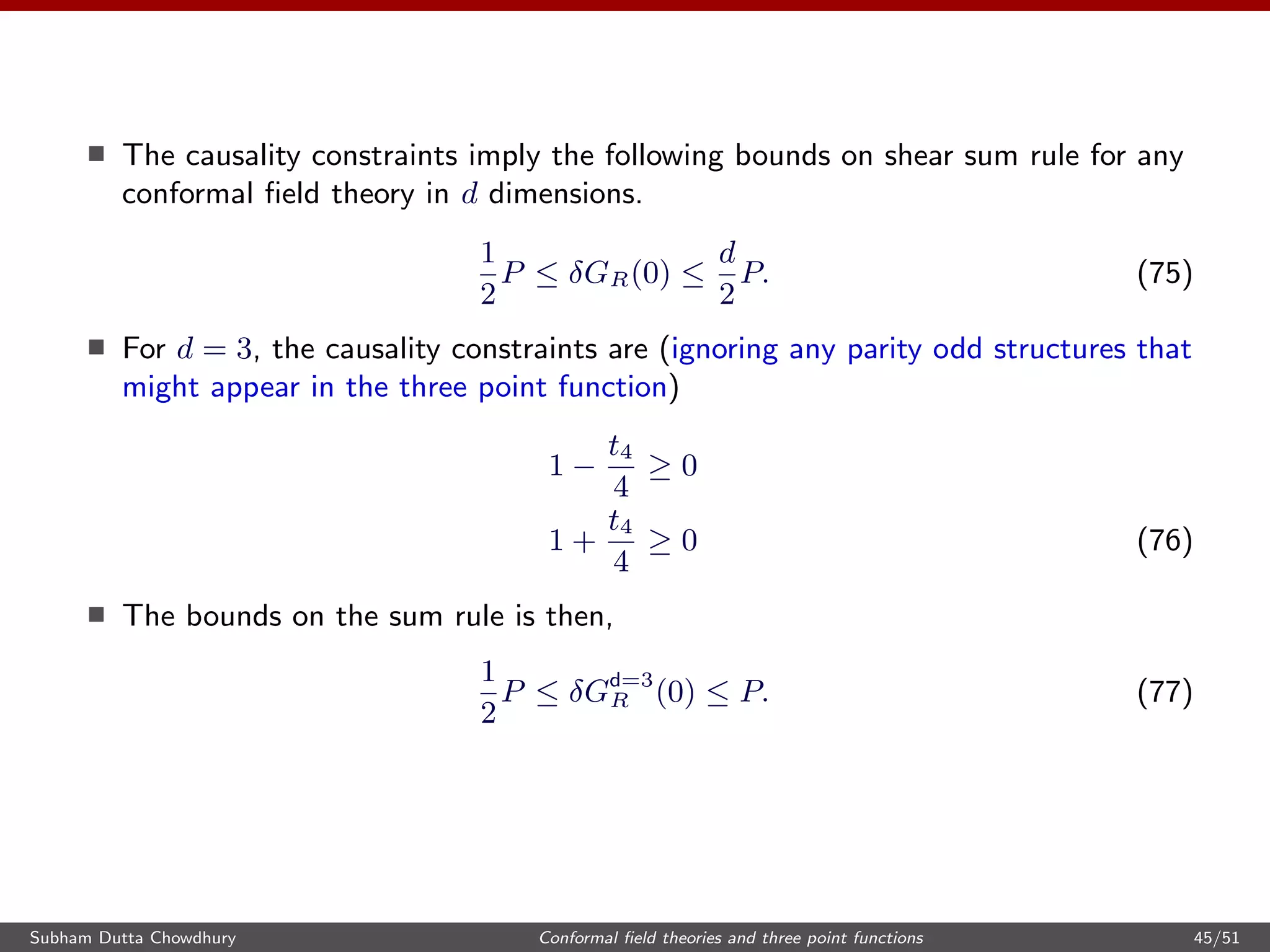
![Sum rules in higher derivative gravity
We can perform similar analysis for gauss bonnet gravity theories in d = 5
(fourth order in derivatives).
The holographic sum rule, obtained by solving a modified minimally coupled
scalar equation, becomes
δG(0) =
6
5
+ 2 1 −
1
√
1 − 4λGB
P (79)
This is consistent with the sum rule that we have derived, with the following
values for t2 and t4
t4 = 0, t2 =
24f∞λGB
1 − 2f∞λGB
(80)
where,
f∞ =
1 −
√
1 − 4λGB
2λGB
(81)
[Buchel et al 2009]
Can be generalised to a generic higher derivative theory (fourth order in
derivatives) in arbitrary dimensions. This will serve as a non trivial check of the
coefficient of t2 in our sum rule.
Subham Dutta Chowdhury Conformal field theories and three point functions 48/51](https://image.slidesharecdn.com/uchicago-171113135150/75/Conformal-field-theories-and-three-point-functions-48-2048.jpg)


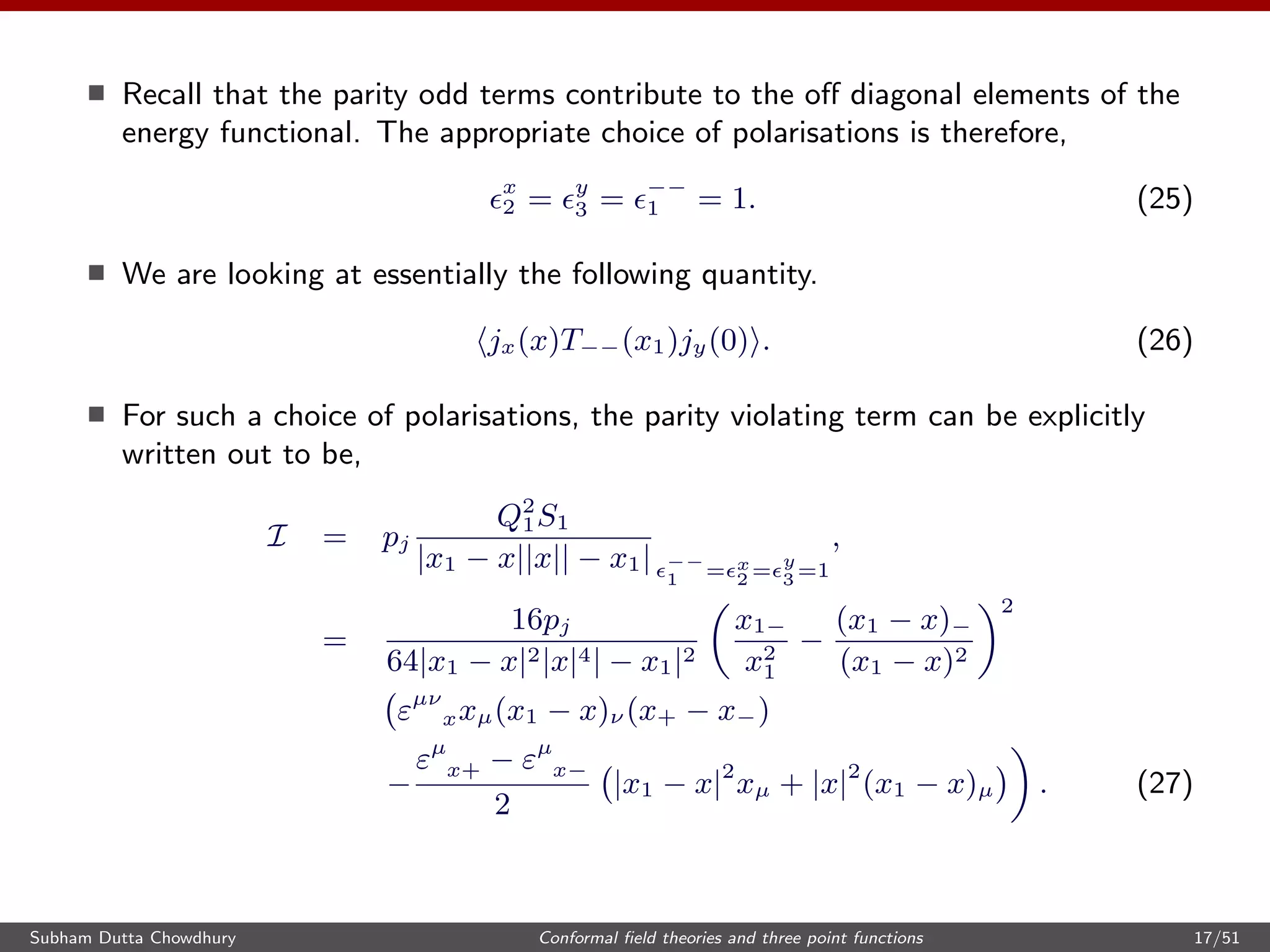
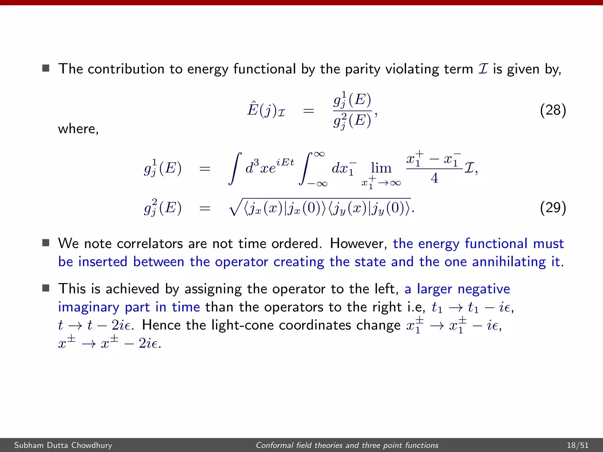
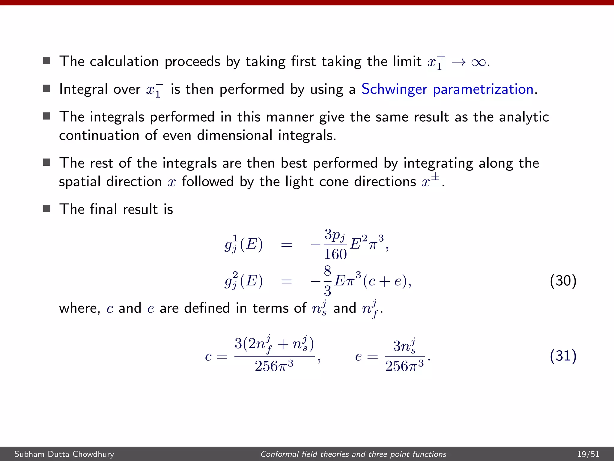
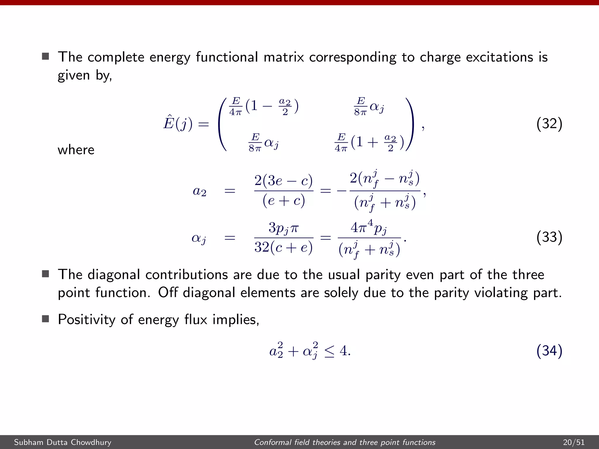
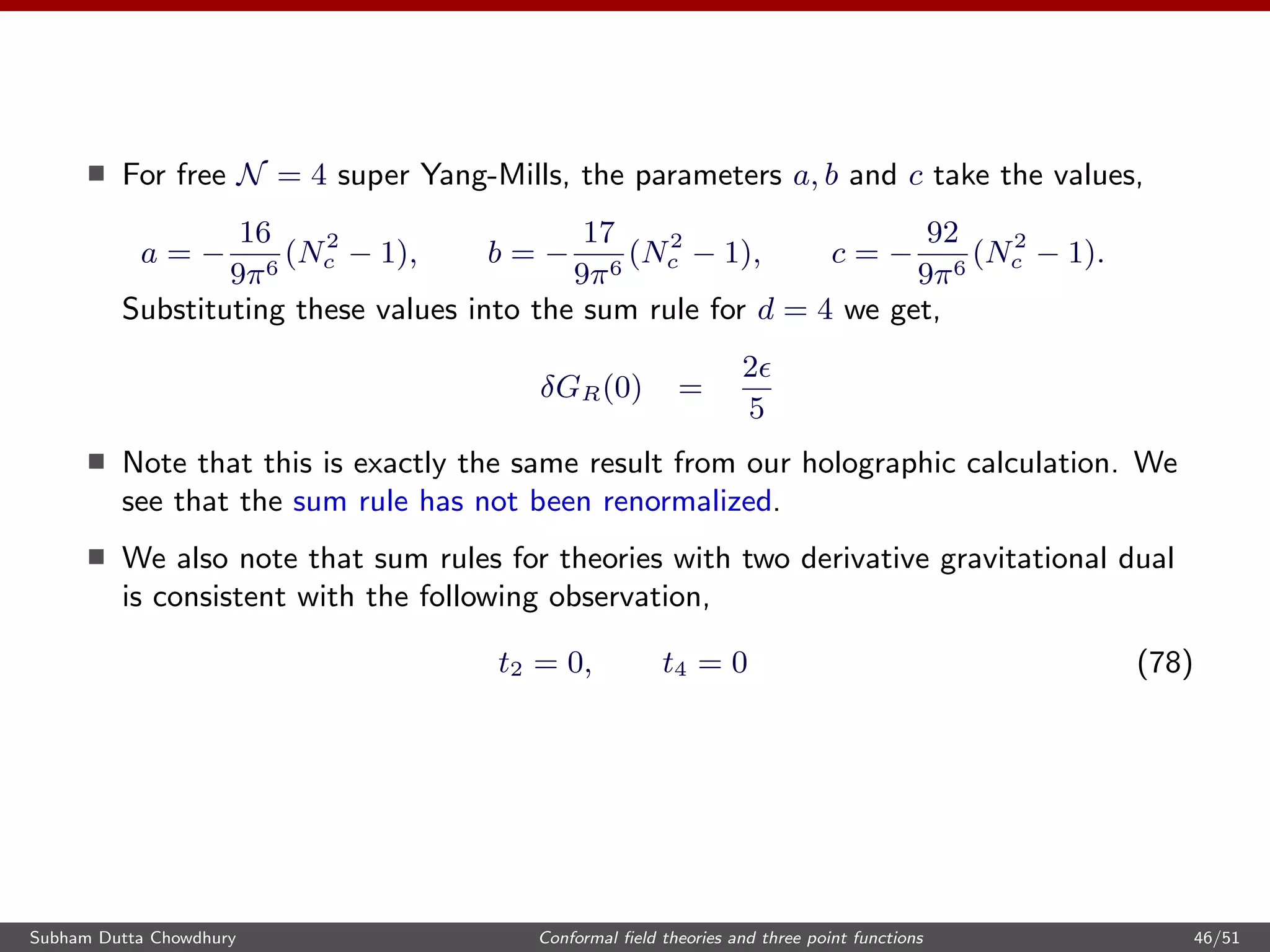
This document discusses conformal field theories and three point functions. It begins by introducing conformal field theories and noting that three point functions of stress tensors are constrained by conformal invariance. For parity even CFTs in d=4 dimensions, the three point functions of the stress tensor T can be written in terms of coefficients that correspond to effective numbers of scalars, fermions, and vectors. Positivity of energy flux from collider experiments imposes constraints on these coefficients. The document then discusses extending such analyses to parity violating CFTs in d=3 dimensions, where the three point functions of the stress tensor T and conserved current j contain both parity even and odd terms. It proposes studying modifications to existing constraints from applying coll


