SlideShare a Scribd company logo
1 of 205
Download to read offline
University of Louisville
ThinkIR: The University of Louisville's Institutional Repository
Electronic Theses and Dissertations
12-2016
Dynamic warehouse optimization using predictive analytics.
Parvaneh Jahani
University of Louisville
Follow this and additional works at: https://ir.library.louisville.edu/etd
Part of the Industrial Engineering Commons, Other Operations Research, Systems Engineering and
Industrial Engineering Commons, and the Systems Engineering Commons
Recommended Citation
Jahani, Parvaneh, "Dynamic warehouse optimization using predictive analytics." (2016). Electronic Theses
and Dissertations. Paper 2582.
https://doi.org/10.18297/etd/2582
This Doctoral Dissertation is brought to you for free and open access by ThinkIR: The University of Louisville's
Institutional Repository. It has been accepted for inclusion in Electronic Theses and Dissertations by an authorized
administrator of ThinkIR: The University of Louisville's Institutional Repository. This title appears here courtesy of the
author, who has retained all other copyrights. For more information, please contact thinkir@louisville.edu.
DYNAMIC WAREHOUSE OPTIMIZATION USING
PREDICTIVE ANALYTICS
By
Parvaneh Jahani
M.S. in Industrial Engineering, Sharif University of Technology, 2012
B.S in Textile Engineering, Tehran Polytechnic, 2009
A Dissertation
Submitted to the Faculty of the
J. B. Speed School of Engineering of the University of Louisville
in Partial Fulfillment of the Requirements
for the Degree of
Doctor of Philosophy in Industrial Engineering
Department of Industrial Engineering
University of Louisville
Louisville, Kentucky
December 2016
DYNAMIC WAREHOUSE OPTIMIZATION USING
PREDICTIVE ANALYTICS
By
Parvaneh Jahani
M.S. in Industrial Engineering, Sharif University of Technology, 2012
B.S in Textile Engineering, Tehran Polytechnic, 2009
A Dissertation Approved On
November 30, 2016
by the following Dissertation Committee:
Professor Kevin R. Gue, Dissertation Director
Professor John S. Usher
Professor Gail W. Depuy
Professor Olfa Nasraoui
ii
ACKNOWLEDGEMENTS
First and foremost, I would like to express my special appreciation and thanks
to my advisor Dr. Kevin Gue. He has always been a tremendous mentor and a
model of a critical, elegant thinker for me. I have been very fortunate to be trained,
instructed, and grounded in his thorough knowledge of warehousing and logistics. I
wish I could have absorbed a fraction of his knowledge in these years. I owe him an
enormous debt of gratitude. His advice on both research as well as on my career have
been invaluable. I also would like to thank his PhD advisor Dr. John Bartholdi who
took the time to listen to our dynamic slotting idea in the early stages and provide
valuable advice.
I am greatly appreciative of my committee members: Dr. John Usher, Dr. Gail
Depuy, and Dr. Olfa Nasraoui. They have provided their insights and suggestions,
which are precious to me. I am grateful to Dr. Suraj Alexander, the chair of the
Industrial Engineering Department, for his help in the demand forecasting chapter.
My sincere thanks also goes to my industrial supporters at Intelligrated, Luther
Webb, Chris Arnold and Mark Steinkamp, who kept me inspired. I was continually
amazed by working with their brilliant team, Operation and Solution Development.
Finally, I would like to thank and dedicate this dissertation to my compassion-
ate and supportive parents Assadollah Jahani and Zahra Karamirad, who experienced
all of the ups and downs of my research via Skype. I undoubtedly could not have
done this without you, your love, and encouragement.
iii
ABSTRACT
DYNAMIC WAREHOUSE OPTIMIZATION USING
PREDICTIVE ANALYTICS
Parvaneh Jahani
November 30, 2016
A warehouse is a key component of a logistics system that provides a central
location for receiving, storing, and distributing raw materials or manufactured goods.
While the objective of a logistics system is reducing the overall inventories and cycle
times (the average time between successive deliveries), warehouses are concerned with
having the right items, available at the right place, at the right time.
As e-commerce continues to expand and order shipments become smaller, more
diverse, and frequent, warehouses must adjust proactive approaches for order fulfill-
ment. Efficient replenishment of the right products into the forward picking areas
becomes a more challenging problem in this dynamic environment. The set of items
ordered in one month might be completely different from next month’s orders. His-
torical time-based demand data provides valuable information for the models, which
have demand as an input. Disregarding the knowledge about the order data behavior
over time is costly. One warehousing problem that is highly dependent on product
demand and picks is the Forward-Reserve Problem (FRP).
iv
The forward area is a small area of a warehouse with a low picking cost.
Therefore, the items of a warehouse compete to be located in this area rather than the
reserve area, which has a higher picking cost. Two approaches that are investigated
for selecting the SKUs of the fast picking area and the allocated space are the static
and the dynamic approaches.
In the case that decisions about the forward area are made periodically (e.g.
yearly) and the products’ demand patterns are completely ignored, the FRP is static.
Due to the NP-hard nature of the product assignment to the forward area, we de-
veloped two heuristics that solve the large discrete assignment, allocation, and sizing
problem simultaneously. We also developed a heuristic that determines the best sizes
of the different pick modes within the forward area.
Using a fixed number for the “demand per year” in the static approach does not
accurately capture the characteristics of the demand pattern. Replenishing the same
product in the same place of the forward area brings about a “Locked” layout of the
fast picking area during the planning horizon. By using a dynamic slotting approach,
the product pick locations within the warehouse are allowed to change and pick oper-
ations can accommodate the variability in the product demand pattern. A dynamic
approach can introduce the latest fast movers to the forward area, as an opportunity
arises, and stop the replenishment of the products with decreasing turnover rates in
this area at the right time. The allocated space to the items in the forward area can
also vary over time. We show that on average 39% of the candidate SKUs for the
forward area experience the flexibility that the dynamic slotting approach provides.
However, updating the forward area periodically in the static approach affect on only
6% of the SKUs.
The primary objective of this dissertation is to formally define the dynamic
v
FRP. Although real-time order picking and replenishment systems are becoming a
pivotal component of today’s order fulfillment systems, no consensus in the literature
has been made regarding a definition for dynamic slotting optimization. One main
mission of this research is to define a generic dynamic slotting problem while also
demonstrating the strengths of this approach over the static model.
Dynamic slotting continuously adjusts the current state of the forward area
with real-time decisions in conjunction with demand predictive analytics. Therefore,
the layout of the fast picking area is updated over time with replenishment of the
appropriate SKUs, as opposed to traditional methods that periodically reslot the
forward area to reach a predefined target map. A powerful slotting methodology
not only considers seasonality, but also other types of demand shifts, trends, and
frequencies. We explored the methods for demand pattern detection and demand
forecasting as well as proposed MIP mathematical model for the dynamic forward-
reserve problem for the first time. This model relaxes the major implicit assumptions
of the static model and quantifies the effects of the static strategy versus the dynamic
strategy.
Extensive numerical experiments are conducted to compare the static FRP so-
lutions, optimal solutions of the dynamic slotting model, and the developed threshold
policy, a faster method that performs almost as well as the dynamic MIP model. The
results show that the threshold policy solution is always very close to the optimal
solution in terms of both the total cost of picking and replenishment and the forward
area assignment and allocation. Applying different order data with different demand
volatility, we show that the dynamic model always outperforms the static model. The
benefits attained from the dynamic model over the static model are greater for more
volatile warehouses.
vi
TABLE OF CONTENTS
Page
ACKNOWLEDGEMENTS iii
ABSTRACT iv
LIST OF TABLES x
LIST OF FIGURES xii
CHAPTER
I INTRODUCTION 1
A Warehousing in logistics systems . . . . . . . . . . . . . . . . . 1
B Warehouse operations . . . . . . . . . . . . . . . . . . . . . . . 2
C Forward-Reserve Operations . . . . . . . . . . . . . . . . . . . . 5
1 Pick mode equipment . . . . . . . . . . . . . . . . . . . . 6
D Forward-Reserve Problem . . . . . . . . . . . . . . . . . . . . . 9
E Literature Review . . . . . . . . . . . . . . . . . . . . . . . . . . 11
F Purpose of the dissertation . . . . . . . . . . . . . . . . . . . . . 14
II THE STATIC FORWARD-RESERVE PROBLEM 18
A Introduction . . . . . . . . . . . . . . . . . . . . . . . . . . . . . 18
B The continuous model for space allocation . . . . . . . . . . . . 19
C A discrete model for space allocation . . . . . . . . . . . . . . . 24
1 Heuristic G1 . . . . . . . . . . . . . . . . . . . . . . . . . 30
2 Testing the model . . . . . . . . . . . . . . . . . . . . . . 31
vii
3 Heuristic G2 . . . . . . . . . . . . . . . . . . . . . . . . . 35
D Comparisons . . . . . . . . . . . . . . . . . . . . . . . . . . . . 43
E Conclusion . . . . . . . . . . . . . . . . . . . . . . . . . . . . . 46
III THE AREA SIZING AND SLOTTING OF A MULTI-MODE FORWARD
AREA 48
1 Extensions . . . . . . . . . . . . . . . . . . . . . . . . . . 58
2 Numerical example with a large data set . . . . . . . . . 63
A Conclusion . . . . . . . . . . . . . . . . . . . . . . . . . . . . . 64
IV DEMAND FORECASTING 68
A Qualitative model . . . . . . . . . . . . . . . . . . . . . . . . . . 69
B Model . . . . . . . . . . . . . . . . . . . . . . . . . . . . . . . . 75
1 Autoregressive Integrated Moving Average (ARIMA) . . 78
2 The bootstrapping method for intermittent demand data 83
V THE DYNAMIC FORWARD-RESERVE PROBLEM 88
A Literature Review . . . . . . . . . . . . . . . . . . . . . . . . . . 91
B Mathematical Model . . . . . . . . . . . . . . . . . . . . . . . . 94
1 The generic MIP model of DFRP . . . . . . . . . . . . . 97
C Numerical example . . . . . . . . . . . . . . . . . . . . . . . . . 99
D Comparison of the static and the dynamic models with multiple
runs of the static model . . . . . . . . . . . . . . . . . . . . . . 103
E Model enhancement . . . . . . . . . . . . . . . . . . . . . . . . 110
F Replenishment policies . . . . . . . . . . . . . . . . . . . . . . . 113
1 Quantity replenishment (M1
) . . . . . . . . . . . . . . . 114
2 Full replenishment (M2
) . . . . . . . . . . . . . . . . . . 116
viii
G Heuristics for the dynamic forward-reserve problem (T.P) . . . 121
H Model Validation and Numerical Discussions . . . . . . . . . . . 122
1 Comparison of the static and dynamic models using the
forecast demand data . . . . . . . . . . . . . . . . . . . . 123
2 Comparison of different replenishment strategies of the dy-
namic model, static model and threshold policies . . . . 124
3 Volatility . . . . . . . . . . . . . . . . . . . . . . . . . . . 132
I Checking the robustness of the models . . . . . . . . . . . . . . 146
1 Sensitivity analysis . . . . . . . . . . . . . . . . . . . . . 148
2 Statistical comparison of the models . . . . . . . . . . . . 158
3 Effects of the size of normal patterns in order data . . . . 159
J Conclusion . . . . . . . . . . . . . . . . . . . . . . . . . . . . . 166
VI SUMMARY 167
REFERENCES 171
APPENDIX 178
CURRICULUM VITAE 187
ix
LIST OF TABLES
TABLE Page
1 Comparisons of the different types of pick mode racks . . . . . . . . . 7
2 Heuristics DFRAAPES −R4, G1 and continuous space model comparisons 32
4 Cost comparisons between the procedures A1 to A4 using heuristic G2 43
5 Comparison of two methodologies for the discrete forward-reserve prob-
lem . . . . . . . . . . . . . . . . . . . . . . . . . . . . . . . . . . . . . 45
7 Inputs . . . . . . . . . . . . . . . . . . . . . . . . . . . . . . . . . . . 54
8 6 possible case orientations in slot . . . . . . . . . . . . . . . . . . . . 55
9 Outputs . . . . . . . . . . . . . . . . . . . . . . . . . . . . . . . . . . 57
10 Rack information . . . . . . . . . . . . . . . . . . . . . . . . . . . . . 58
11 Experiments for pick mode analysis . . . . . . . . . . . . . . . . . . . 64
12 The ARIMA model results for instances of demand trends classes of 1
through 7 . . . . . . . . . . . . . . . . . . . . . . . . . . . . . . . . . 82
13 Summary statistics for intermittent demand forecasting . . . . . . . . 86
14 The values of model’s parameters . . . . . . . . . . . . . . . . . . . . 102
15 Results of cost and solution time comparisons of the static versus dy-
namic model . . . . . . . . . . . . . . . . . . . . . . . . . . . . . . . . 102
16 Picking and replenishment cost for the static model. . . . . . . . . . . 107
17 The number of different SKUs (DSKi) and the different slots (DSLi)
in the previous and next states of the forward area in a static model . 108
18 Cost of moving to reserve area in the static model . . . . . . . . . . . 108
x
19 The total cost and savings (%) obtained from the static and dynamic
models (PI). . . . . . . . . . . . . . . . . . . . . . . . . . . . . . . . 109
21 Total cost and savings (%) obtained from static(S) and dynamic model
M2
a . . . . . . . . . . . . . . . . . . . . . . . . . . . . . . . . . . . . . 124
22 Cost comparisons of the activity distribution of items (M2
a ) . . . . . . 125
23 Results for different replenishment policies of DFRP . . . . . . . . . . 128
24 No. of SKUs with different values of Ki . . . . . . . . . . . . . . . . . 131
25 Example for the volatility index calculation . . . . . . . . . . . . . . . 136
26 Comparison of the dynamic model, threshold policies T.P. and T.P.0
and static model for warehouses with different portion of SKUs with
normal demand pattern . . . . . . . . . . . . . . . . . . . . . . . . . . 141
27 Factors and levels in experimental design . . . . . . . . . . . . . . . 148
28 Full factorial design 26
. . . . . . . . . . . . . . . . . . . . . . . . . . 150
29 Summary of the main effects of the models . . . . . . . . . . . . . . . 157
33 Costs for the data set with 10% Normal demand patterns . . . . . . . 183
34 Costs for the data set with 30% Normal demand patterns . . . . . . . 184
35 Costs for the data set with 50% Normal demand patterns . . . . . . . 185
36 Costs for the data set with 70% Normal demand patterns . . . . . . . 186
xi
LIST OF FIGURES
FIGURE Page
1 Basic flows in a warehouse . . . . . . . . . . . . . . . . . . . . . . . . 3
2 Bay configuration . . . . . . . . . . . . . . . . . . . . . . . . . . . . . 3
3 Structure of an SKU . . . . . . . . . . . . . . . . . . . . . . . . . . . 4
4 Pallet flow rack . . . . . . . . . . . . . . . . . . . . . . . . . . . . . . 6
5 Carton flow rack . . . . . . . . . . . . . . . . . . . . . . . . . . . . . 8
6 Decked rack . . . . . . . . . . . . . . . . . . . . . . . . . . . . . . . . 8
7 Steel shelving . . . . . . . . . . . . . . . . . . . . . . . . . . . . . . . 8
8 Bin shelving . . . . . . . . . . . . . . . . . . . . . . . . . . . . . . . . 9
9 The sorted ACI and ACD for 100 replications . . . . . . . . . . . . . 34
10 The unavoidable wasted empty space due to the difference between the
cases and the allocated slots dimensions. . . . . . . . . . . . . . . . . 37
11 The cost reduction representation with increasing the number of SKUs
in forward area. . . . . . . . . . . . . . . . . . . . . . . . . . . . . . . 41
12 The bottom-up deletion approach. . . . . . . . . . . . . . . . . . . . . 42
13 The cost comparisons of G2 using different scenarios A1 to A4. . . . . 44
14 Heuristic G2 − A1 for real world data set with 6498 SKUs. . . . . . . 45
15 The multi-mode forward area . . . . . . . . . . . . . . . . . . . . . . 50
16 Pick mode cost for experiments 1 through 6 . . . . . . . . . . . . . . 65
17 Carton flow rack and bin shelving comparison . . . . . . . . . . . . . 66
18 Demand trend shown by Control Chart . . . . . . . . . . . . . . . . . 70
xii
19 Basic structure of a NN . . . . . . . . . . . . . . . . . . . . . . . . . 71
20 Example of different generated demand patterns. . . . . . . . . . . . 74
21 Confusion matrix for demand trend classifier. . . . . . . . . . . . . . 76
22 Error Histogram for demand trend classifier. . . . . . . . . . . . . . . 77
23 Algorithm of demand forecasting . . . . . . . . . . . . . . . . . . . . 81
24 Algorithm for forecasting the intermittent demand data . . . . . . . . 85
25 The run procedure for the dynamic slotting model . . . . . . . . . . . 100
26 The planning horizon diagram with different run intervals for the test
example . . . . . . . . . . . . . . . . . . . . . . . . . . . . . . . . . . 105
27 The planning horizon diagram with different run intervals . . . . . . . 106
28 Warehouse layout (Forward area: green aisles; Reserve area: black aisles)111
29 Replenishment policies . . . . . . . . . . . . . . . . . . . . . . . . . . 117
30 ABC analysis . . . . . . . . . . . . . . . . . . . . . . . . . . . . . . . 126
31 Number of moves from the forward area to reserve area . . . . . . . . 130
32 Distribution of SKUs with different values of Ki . . . . . . . . . . . . 133
33 The curves corresponded to the Table 25 . . . . . . . . . . . . . . . . 137
34 The volatility curve of the numerical example . . . . . . . . . . . . . 137
35 Volatility diagrams of simulated order data 1 through 6 . . . . . . . . 139
36 Volatility diagrams of simulated order data 7 through 10 . . . . . . . 140
37 Dynamic model efficiency versus the demand volatility . . . . . . . . 142
38 Demand volatility impacts on picks from the forward or reserve area . 143
39 Demand volatility impacts on the total replenishments and moves . . 144
40 Demand volatility impacts on the total cost . . . . . . . . . . . . . . 145
41 ANOVA1
test for the static model . . . . . . . . . . . . . . . . . . . . 149
42 ANOVA2
test for the static model . . . . . . . . . . . . . . . . . . . . 151
xiii
43 Normal Probability Plot for the static model . . . . . . . . . . . . . . 151
44 ANOVA1
test for the T.P. model . . . . . . . . . . . . . . . . . . . . 152
45 ANOVA2
test for the T.P. model . . . . . . . . . . . . . . . . . . . . 152
46 Normal Probability Plot for the T.P. model . . . . . . . . . . . . . . 153
47 ANOVA1
test for the T.P.’ model . . . . . . . . . . . . . . . . . . . . 153
48 ANOVA2
test for the T.P.’ model . . . . . . . . . . . . . . . . . . . . 154
49 Normal Probability Plot for the T.P.’ model . . . . . . . . . . . . . . 154
50 ANOVA1
test for the dynamic model . . . . . . . . . . . . . . . . . . 155
51 ANOVA2
test for the dynamic model . . . . . . . . . . . . . . . . . . 155
52 Normal Probability Plot for the dynamic model . . . . . . . . . . . . 156
53 ANOVA table for comparison of the models . . . . . . . . . . . . . . 159
54 Box plot of the costs for four models . . . . . . . . . . . . . . . . . . 160
55 ANOVA table for significance of the normal patterns portion in the
order data (static model) . . . . . . . . . . . . . . . . . . . . . . . . . 161
56 Box plot for significance of the normal patterns portion in the order
data (static model) . . . . . . . . . . . . . . . . . . . . . . . . . . . . 162
57 ANOVA table for significance of the normal patterns portion in the
order data (T.P. model) . . . . . . . . . . . . . . . . . . . . . . . . . 162
58 Box plot for significance of the normal patterns portion in the order
data (T.P. model) . . . . . . . . . . . . . . . . . . . . . . . . . . . . . 163
59 ANOVA table for significance of the normal patterns portion in the
order data (T.P.0
model) . . . . . . . . . . . . . . . . . . . . . . . . . 163
60 Box plot for significance of the normal patterns portion in the order
data (T.P.0
model) . . . . . . . . . . . . . . . . . . . . . . . . . . . . 164
xiv
61 ANOVA table for significance of the normal patterns portion in the
order data (dynamic model model) . . . . . . . . . . . . . . . . . . . 164
62 Box plot for significance of the normal patterns portion in the order
data (dynamic model) . . . . . . . . . . . . . . . . . . . . . . . . . . 165
xv
CHAPTER I
INTRODUCTION
A Warehousing in logistics systems
A warehouse is a building used for the storage of goods, such as manufactured
parts, raw materials, spare parts and more. This building has both receiving and
shipping areas, in which goods are unloaded from the trucks in the receiving docks
and are loaded to the trucks on a smaller scale in the shipping docks. The level of
automation differs in different warehouses. While the products are completely picked,
packed, and transported automatically in some warehouses, others utilize labor for
those activities.
Material flow within the warehouse varies in terms of both type of Stock Keep-
ing Units (SKUs) and the volume. SKUs and demand growth are two subjects that
jeopardize any warehouse space management system. These growths will also affect
warehouse functions. In some cases, managers must accommodate by adding new
products to the already strained capacity of the distribution center. They may also
need to apportion available space to those SKUs that have experienced growth in
demand.
Every warehouse requires labor, capital, land, and an information system, but
providing these resources is costly. One important reason to have a warehouse is to
address a highly volatile and changing demand environment. Warehouses provide a
1
buffer for these unpredictable changes. They can also reduce transportation costs
by product consolidation before shipping the aggregate volume. Several value added
services, such as packaging, returned product services, repairs, testing, inspection,
and assembly, are provided by warehouses.
B Warehouse operations
To accomplish the broad scope of warehousing functions (e.g. receiving, stor-
ing, picking, sorting, packing, shipping), a warehouse is commonly divided into several
functional areas. Figure 1 illustrates the basic flows in a warehouse, starting from
the receiving area and ending in the shipping area. After products are received, they
are sent to other functional area(s) or directly to the shipping area. The process
of unloading the receiving trucks and directly loading the shipping trucks is called
cross-docking.
Warehouse operations are labor intensive. Bartholdi and Hackman (2010)
report that 55% of warehouse operating costs belong to order-picking. This shows
the high potential of order picking and replenishment for warehouse improvements.
Not all of the areas of a warehouse have the same picking cost, however, the larger
areas and also the farther areas from the Input/Output (I/O) point have a larger
picking cost because pickers have to travel longer distances to pick items.
Slot and slotting are two common terms in warehouse studies. A slot is the
place allotted to the products on the shelf (see Figure 2). The front side view of Figure
2 shows three bays, each having three shelves with four slots per shelf. Slotting is the
process of determining the item location in a warehouse.
Regarding SKU units, we use the same terms applied in Walden (2005). Figure
3 illustrates the unit levels that describe an SKU in a warehouse. The levels are
2
Figure 1. Basic flows in a warehouse
Figure 2. Bay configuration
3
pallet, tier (level), case (carton), inner, and each (piece), respectively. As Figure 3
demonstrates, a pallet includes layers of cartons. In logistics industry, the number of
cartons on a layer is called TI. The number of layers that are stacked on the pallet is
called HI. The TI and HI values in Figure 3 are 15 and 6, respectively. Case refers to
the carton or box. A quantity per pick is usually less than a full case. The smallest
unit of the SKU, which is picked from inside of the case, is called an each or piece.
Figure 3. Structure of an SKU
While some zones of the warehouse are replenished by the SKU cases, others
can be replenished by the pallets. Likewise, the SKUs can be picked by units or
cases. The information about the SKUs and cases such as the length, the width, the
height, the weight, the case pack (the number units per case), and the order data
affect the warehouse operation decisions. An item in the warehouse can have a single
or multiple pick location(s). The products are scanned in the different functional
areas for tracking and visibility purposes. Determining the best pick location(s) of
the products in the warehouse is challenging. Searching and extracting the SKUs
located in the smaller areas need less travel distance. However, the picker should
travel more distance to find and pick an item from the larger areas.
4
C Forward-Reserve Operations
The forward area, or the fast picking area, is a small valuable section of the
warehouse with low picking cost. It is expected that the distance the picker traverses
in the forward area to pick an order is less than the distance traversed in the reserve
area because the forward area is smaller than the reserve area. In addition, the
physical nature of rack types in the forward area that we discussed earlier make the
pick operation more convenient in the forward area.
The items that go into the forward area are replenished (restocked) from the
reserve or bulk area, which is a large area with a high picking cost, to be picked more
efficiently. The SKUs are scheduled to be replenished from the reserve area to the
forward area. The Warehouse Management System (WMS) keeps track of real-time
inventory and schedules the replenishments. The best utilization of the areas with
low picking costs plays a significant role in having a more productive warehouse.
The total picking and replenishment costs will increase considerably if we
choose a wrong set of SKUs for the forward area. The reason is that inappropri-
ate SKU assignment results in less saving opportunities that the forward area can
provide. In addition, the number of replenishments will rise if the allocated slot(s) to
the SKUs in the forward area is less than optimal. Allocating more slots than optimal
reduces the chance of having a larger set of SKUs in the fast picking area. A clever
approach to detect the best SKU for the fast picking area and also the optimal slot
allocation enhances warehouse productivity and reduces operational costs.
Since the cost of picking from the forward area is low, one may be inclined to
have more products in the forward area due to the low picking cost. Two strategies
lead to having more items in the forward area: enlarging the forward area, and
5
allocating less space to each item. The first approach often increases the picking cost,
since the picker has to travel a longer distance to pick. The second approach not
only involves more items in the restocking process, but also increases the number of
replenishments from the reserve area to satisfy the demand. The optimal size of the
forward area reduces the total cost of picking and replenishments.
1 Pick mode equipment
To present more details about the pick modules in the forward area, we compare
different types of pick modes in this section. The term pick mode refers to a region of
the forward area with similar rack characteristics. Typical examples of pick modes in
the forward area include five categories: pallet flow racks, carton flow racks, decked
racks, steel shelving, and bin shelving. Table 1 compares these different types of racks
shown in Figures 4, 5, 6, 7, and 8.
Figure 4. Pallet flow rack
6
TABLE 1
Comparisons of the different types of pick mode racks
Pallet flow rack
Application Used for the fastest movers.
Advantage
Can hold a substantial amount of inventory for a single SKU.
Fast replenishment.
Replenishment does not interfere with picking.
Disadvantage
Low SKU density.
Can pass few SKU’s in a long distance.
Low space utilization.
Carton flow rack
Application Used for fast to medium movers.
Advantage
Can be replenished by the behind reserve racks.
Can hold a substantial amount of inventory and minimize the linear travel.
Replenishment does not interfere with picking.
Disadvantage
Low cube utilization.
Density is lower than steel shelving and more expensive than it.
Smaller product falls through the skate wheels or rollers.
Decked rack
Application Used for medium to slow movers.
Advantage
Can be utilized on the floor level with reserve pallets above.
Medium SKU density.
Disadvantage
Higher cost.
Decked rack has a thick support beam compared to shelving.
Steel shelving
Application Used for slow movers.
Advantage
High SKU density.
Can pass many SKUs in a short distance.
High space utilization
Disadvantage
Not ideal for larger SKUs.
Replenishment is cumbersome.
Bin shelving
Application Used for small slow movers.
Advantage
Low cost.
High space utilization.
Disadvantage
Can result in excessive travel for a picker.
Difficult to pick from the top shelf.
Replenishment can interfere with picking.
7
Figure 5. Carton flow rack
Figure 6. Decked rack
Figure 7. Steel shelving
8
Figure 8. Bin shelving
D Forward-Reserve Problem
The literature on the forward-reserve problem so far assumes that a warehouse
has one small and one large section, named fast and slow picking areas, respectively.
In practice, the fast picking area may refer to a shelving area, a section of the carton
flow rack, or even an automated system, such as carousels or a miniload system. Our
research is not concerned with the specific type of system as long as the picking cost
within the area is lower than in the reserve area.
To clarify the configuration of the forward-reserve area in this dissertation, we
describe our system as:
The warehouse has a forward and reserve area, where the picking cost from
the forward area is less in the reserve area, and the restocking cost from the reserve
area to the forward area is more than the cost of picking from the reserve area.
Assuming that the item is available in the reserve area, we perform concurrent
replenishment, in which the replenishments can happen during the order picking
process.
As opposed to a storage/retrieval machine that travels along the aisle to bring
part(s) to the picker, our picking policy in both the forward and reserve areas is
9
picker-to-parts, where the order picker walks or drives along the aisles to pick order
lines.
Only one SKU can be stored in a particular slot.
Optimizing the decisions about the forward area is addressed in a well-known
warehousing problem called the Forward-Reserve Problem (FRP). Two important de-
cisions of this problem are the selection and the quantities of SKUs in the forward
area. The size of the forward area is another critical decision. All previous studies
assume that the set of SKUs assigned to the forward area should be known to deter-
mine the appropriate size of the forward area. The research in this dissertation solves
these three problems simultaneously.
The decisions about the forward and reserve areas are critical. Selecting the
wrong products for the forward area is costly. If the slow movers are stored in the
forward area, the chance of having more fast movers in the fast picking area is reduced.
If the fast movers with high volume movement per year are selected for this area, the
slots of the fast picking area will be depleted frequently and having enough inventory
for pick operations will require more restocks.
In addition, if the allocated slots to the SKUs in the forward area are higher
than the optimal, we can store less products there and so less savings by picks will
be achieved. If the allocated slots are less than optimal, it will result in more re-
plenishments. The picking and replenishment costs in the forward-reserve problem
can significantly increase with improper SKU assignment and slot allocation. The
mathematical models for the traditional forward-reserve problem will be presented in
section B of Chapter II.
10
E Literature Review
The static forward-reserve problem with a continuous allocation of space has
been widely researched. Hackman et al. (1990) were the first to develop a mathemat-
ical model for the problem. They proposed a greedy heuristic to solve the model. A
further contribution is Frazelle et al. (1994), which considers the size of forward area
as the decision variable.
Gu et al. (2010) applies a branch and bound algorithm to solve the forward-
reserve problem. They assert that the heuristic and optimal assignment of SKUs, as
well the total cost, are very close together. The optimal stocking strategy is analyzed
by Bartholdi and Hackman (2008) and Bartholdi and Hackman (2010) in detail. They
compare the optimal strategy with two practical real world strategies: equal space
and equal time allocations. Equal space allocation strategy allocates the same amount
of space to each SKU. Equal time allocation strategy allocates an equal time supply
of each SKU in the forward area.
Hackman and Platzman (1990) extend the fluid model by proposing a generic
discrete model based on non-smooth convex relaxation for determining the SKUs and
their volume, in an automated forward area. They develop an algorithm with near-
optimal solution for the problems, where each allocation is a fraction of standard size
bin. One deficiency of the greedy heuristic is that it provides no posterior bound on
the performance of the solution (Hackman and Platzman, 1990).
Walter et al. (2013) relax the assumption of continuous space forward area and
solve the discrete assignment, allocation, and sizing of the fast picking area. However,
they do not solve these three problems simultaneously. They propose four heuristics
for solving the discrete forward-reserve problem, which allocates SKUs to shelves (in
11
contrast with slots). Their method is applicable for small size problems. We address
this study in chapter II in detail.
Van den Berg et al. (1998) investigate the prior to picking replenishments to
minimize the expected labor during the pick period, assuming that prior to pick-
ing period there is sufficient time for replenishing the products. They consider the
replenishments and demands of forward area SKUs as random variables. Through
this method, the number of restocks in objective function of problem Continuous
Assignment-Allocation Problem (CAA) is no longer nonlinear. They perform a con-
current replenishment of unit load of SKU i. In other words, their model determines
whether the unit load of an SKU is replenished prior to picking period or not. The
number of restocks in their model is defined as the sum of the multiplication of binary
decision variables (xij: if the jth unit-load of SKU i is replenished in advanced or
not) by the probabilities of having more demand of SKU i than j allocated unit loads.
They solve the linear programming relaxation of the discrete model and obtained lim-
ited number of fractional solution.
Bozer (1985) discusses the optimal inventory and unit load size in the picking
area. He also compares the results of considering the entire warehouse as picking area
and separating the picking and reserve areas.
Heragu et al. (2005) investigate the proportion of continuous available space
allocated to forward, reserve, and cross-docking areas. They consider five operation
areas in the warehouse: receiving, shipping, forward area, reserve area, and cross-
docking operation. The authors define four material flows based on these configura-
tions, where all originate from the receiving area and end in the shipping area. The
first flow involves a cross-docking operation. Order picking is performed directly from
the reserve area in the second flow. The third flow is similar to the forward-reserve
12
problem environment. The last flow stores the product directly in the forward area
to perform order consolidation. This research assumes that the product assignment
of each area is known. In addition, the average distance traveled to store and retrieve
a product in an area is constant and also known. Finally, the model decides whether
or not a product should be assigned to a flow, and how much space is to be allocated
to each functional area.
Hollingsworth (2003) reduces the number of restocks by performing replenish-
ments directly from the receiving area. It minimizes the replenishment cost containing
three components: the number of trips from receiving area to reserve area, the num-
ber of trips from reserve area to forward area, and the number of trips from receiving
area to forward area. In the domain of restocking cost reduction, Liu et al. (2011)
develop a non-linear mathematical fluid model for allocation of storage resources in
the forward area. Their order picking system, called the Complex Automated Order
Picking System (CAOPS), is automated with multiple dispenser types. They consider
four storage modes and safety stocks for each mode.
Some researchers have studied replenishment prioritization of the forward area.
Gagliardi et al. (2008) propose four heuristics for replenishment policies, two for long-
term demand, and two for short-term demand. Unlike Gagliardi et al. (2008) that
study the replenishment of the next product, de Vries et al. (2012) consider wave-
picking and set replenishment priorities for several workers. The latter develops two
replenishment strategies. The first one, Stock-Needs Rule, prioritizes the replenish-
ments based on a ratio dividing the available inventory. The second strategy, the
Order-Quantity Based Rule, minimizes the total expected number of zero-picks. The
authors extend their study further by comparing three policies for prioritizing replen-
ishments and considering the number of stockouts (de Vries et al., 2014).
13
In addition to exact optimization techniques and heuristics, the forward reserve
problem can be investigated by simulation methods. Venkatadri et al. (2015) propose
a simulation model to evaluate the queueing of a given product placement policy in
the forward area. This study aims to reduce the congestion in the fast picking area.
We will review the relevant studies to the dynamic slotting optimization prob-
lem in chapter V.
F Purpose of the dissertation
To have the best set of SKUs in the forward area continuously, warehouses
apply the static FRP periodically. This approach prompts inevitable assumptions.
The forward area will have a fixed set of SKUs during a certain period. The products
have only one pick location in the warehouse if they are assigned to the forward area.
In other words, they should be picked only from the forward area, not the reserve
area. However, when the order quantity is occasionally high, it is more efficient to
pick the item from the reserve area rather than the forward area. This assumption
originates from choosing a fixed number as an annual demand of SKU. Furthermore,
refilling the same SKU in the same location with the same replenishment quantity is
not the best way to address the SKUs’ order fluctuations over time. To combat this,
we develop a dynamic model to update the layout of the forward area over time.
We have heard from warehouse managers that they want to avoid the long list
of moves generated after running the FRP. The moves are designated for transferring
the slow movers to the reserve area. They may only need to update specific areas
within their picking area more frequently to keep up with changing demand like
seasonality. The dynamic slotting proposed in this research addresses that need.
Dynamic approach performs the reslotting of the forward area —updating the forward
14
area layout— on a frequent basis by using the replenishment of empty slots with the
correct SKUs without any moves.
Besides, there are critical questions that warehouse managers are challenging
with:
1. Which SKUs go into forward area?
2. How many days of inventory should a restocker store in the forward area?
3. How often should a facility reconsider the set of items that go into the forward
area and allocated slots?
4. If an SKU is stored in the forward area, are there any cases that it can more
efficiently be picked from the reserve area rather than the forward area?
The first two questions have been extensively studied with an assumption of
continuous space of the forward area. The last two questions have not been answered
in literature. The problem addressing the integral solution of assignment, allocation,
and sizing simultaneously, which consider the slot and SKU geometries, have not been
answered yet.
There are two major weaknesses in previous studies on the FRP. First, they
assume that the space of the forward area is continuous, when most often it is dis-
crete. Assuming cubic product movement per year and disregarding slot and SKU
dimensions, they allocate cubic space of the forward area to the selected items for
this area. In addition, current approaches assume decisions about the forward area
are one-time decisions during the planning horizon. As a result the fast picking area
is replenished with the same products for a long time. These approaches miss the
opportunity of updating the layout of the forward area based on the SKUs’ demand
15
patterns over time. SKU assignment and allocation in the fast picking area are not
long term decisions because of the ever-changing demand environment.
The first shortcoming of previous studies creates a gap between the “state of
art” and the “state of practice” in the forward-reserve problem. The state of practice
does not allow allocation of the continuous space of the forward area to SKUs, while
the state of art is based on this assumption. The space wasted while allocating the
SKUs to the slots is unavoidable. Geometry considerations for both slots and SKUs
are necessary. We develop a discrete FRP model, which relaxes these continuous
model assumptions.
The contributions of this dissertation are:
Contribution 1: For the static forward-reserve problem, we develop two heuris-
tics that address the discrete assignment, allocation and the sizing of the forward-
reserve problem for large size problem. As opposed to the first heuristic, the second
heuristic takes the slots and SKUs’ dimensions into account. The algorithms are fairly
simple, fast, and applicable for a real world warehouse. The solutions are quite close
to the optimal.
Contribution 2: We propose an algorithm for both profiling and slotting opti-
mization simultaneously. This algorithm determines the best size of each pick mode
within the forward area, as well as respecting the different rack configurations, pick
technology specifications and replenishment policies of the pick modes. The SKU and
demand growths, the active period of the fast movers based on their order date, and
the optimal case orientation in each slot are the subjects that have also been taken
into consideration.
Contribution 3: To the best of our knowledge, we are the first to propose
the dynamic forward-reserve problem. We developed the first MIP formulation for
16
the dynamic assignment and allocation of the forward area. The main contribution
of this research is quantifying the effects of the traditional wisdom of running the
static model in certain intervals assuming constant demand. We elaborate on de-
mand trend analysis prior to the development of the dynamic forward-reserve model.
We first propose an Artificial Neural Network (ANN) based model for pattern recog-
nition of the different types of demand trends. Further, we develop an algorithm for
forecasting the demand quantity. The method of forecasting is dependent of the class
of demand trend recognized in the previous stage. The algorithm is the combination
of the AutoRegressive Integrated Moving Average (ARIMA) model for predicting
smooth demand trends and the Markov-based bootstrapping method for predicting
intermittent demand pattern.
The remainder of the dissertation has been organized as follows. Chapter II
focuses on static forward-reserve problem and presents two intuitive simple heuristics
for discrete FRP. We propose an algorithm in Chapter III for determining the best
sizes of pick modes within the forward area. A model for predictive analytics of
products’ demand is developed in Chapter IV. We propose the MIP formulation for
the dynamic forward-reserve problem and compare the static and dynamic model
with experimental design in chapter V. Chapter VI concludes the dissertation.
17
CHAPTER II
THE STATIC FORWARD-RESERVE PROBLEM
A Introduction
This chapter addresses the static discrete assignment, allocation, and sizing
problems of the forward area. The term static suggests that the decisions about
the forward area are made periodically (e.g. yearly). This approach disregards the
SKUs’ demand trends during the planning horizon. Thus, in the static forward-
reserve problem, the demand term represents the total demand of an SKU during the
past year or in a forecast year.
The term discrete suggests that discrete units of the SKUs can be stored in
discrete slots. This concept avoids allocating a portion of a slot to an SKU, which
is allowed in the continuous space model but not in practice. Previous research in
this area has focused on the continuous forward-reserve problem. No more than one
type of SKU can be kept in the discrete model. The discrete model considers lost
space resulting from differences in slots and SKU dimensions. Solving the allocation
problem in a continuous space model causes many SKUs having allocated space of
less than one slot, which is impractical.
Rounding down the solution of continuous space model threatens the optimal
solution. It has the risk of removing SKUs with less than one allocated space, from
the forward area. Further, if the case width is larger than the allocated slot(s) width,
18
the stored unit will no longer fit the allocated slot(s).
Rounding up the solution of continuous space model may also assign the inel-
igible slow movers with very small space (close to zero), to the forward area. Con-
sequently, the eligible ones will have to leave the set of SKUs of forward area or
get fewer slots. Allocating few slots will increase the number of replenishments. To
address the aforementioned shortcomings, this chapter tackles the discrete forward-
reserve problem considering both slot and SKU dimensions. There is also the need
for solving the assignment, allocation and sizing problems, simultaneously, for a large
number of SKUs.
B The continuous model for space allocation
The fluid model for space allocation assumes that the forward area can be
continuously subdivided. In other words, each SKU is considered as an incompressible
fluid rather than discrete units that are packed in cartons. Since the solution of the
continuous space model is the basis of our proposed algorithms for the discrete model,
we first review Hackman et al. (1990)’s model for allocation and assignment of SKUs
to the forward area in this section.
The flow rate of SKU i fi is the demand of SKU i per year expressed as volume
per year, e.g. cubic feet per year. Variable fi can be computed as follows (Bartholdi
and Hackman, 2010):
fi =
di
bi
oi, (1)
where di is the demand of SKU i per year (units per year), bi is the number of selling
units within a storage unit (case), and oi is the volume per storage unit of SKU i.
Hackman et al. (1990) assume that the pick quantity for SKU i in the forward
19
area is always less than the full allocation of an SKU in the forward pick area. A
restock is scheduled when the inventory level of slots drop to a certain threshold. The
number of restocks per year is defined as follows:
ri =
&
fi
vi
'
(2)
where vi is the volume of SKU i stored in forward area. In the fluid model, it is also
assumed that the replenishment can be fully satisfied in one trip. In other words, the
entire restock quantity is always less than the restocker capacity. The restocking cost
includes the following costs (Bartholdi and Hackman, 2008):
1. The travel between forward and reserve areas, which depends on the warehouse
layout.
2. The average travel within the reserve area, which is based on “random storage”
in this area.
3. The negligible cost of traveling within the forward area, since the size of forward
area is a small fraction of the warehouse.
4. The fixed cost of handling storage units while restocking.
Due to the fixed and small nature of these cost components, the number of re-
stocks multiplied by the associated restocking cost fully represents the total restocking
cost. Hackman et al. (1990) develop a heuristic solution algorithm, with a priori and
posteriori tests for optimality, to determine which SKUs go into the forward area. In
their model, the space allocated to each SKU is continuous. Their objective function
maximizes the benefits (pick savings, less restock costs) as below.
20
Problem CA (Continuous Allocation Problem):
Maximize
X
i∈A
spi − c
fi
vi
(3)
X
i∈P
vi ≤ V (4)
vi > 0 (5)
where V is the volume of the forward area, pi is number of picks of SKU i per
unit time, A is the set of SKUs that go into forward area, s is the savings per pick if
stored in the forward area (s is equal to the difference between cost of picking from
the reserve area and forward area), and c is restocking cost.
The capacity constraint refers to the maximum inventory of each SKU selected
to be assigned in forward area. Given the set of items allocated to the forward area
and setting optimal Lagrange multiplier for constraint 4, the space allocation vector
v = {v1, ..., vi} can be computed as below (Hackman et al., 1990):
v∗
i =
√
fi
P
i∈A
q
fj
V. (6)
The following knapsack problem considers the allocation and assignment of
SKU i to forward area together.
Problem CAA (Continuous Assignment-Allocation Problem):
Maximize
n
X
i=1
c1pi + c
fi
vi
!
xi +
n
X
i=1
(c2pi)(1 − xi) (7)
n
X
i=1
vixi ≤ V (8)
xi ∈ {0, 1} (9)
21
The reformulation of problem CAA based on ci = c2 − c1 is
Maximize
n
X
i=1
spi − c
fi
vi
!
xi (10)
n
X
i=1
vixi ≤ V (11)
x ∈ {0, 1} (12)
where c1 and c2 are the cost of picking from the forward and reserve areas, respectively,
and xi is the binary decision variable determining if item i is assigned to the forward
(xi = 1) area or not (xi = 0). Problem CAA is NP-complete. A well known heuristic
for solving this category of problem is to rank the SKUs according to their “bang-for-
buck,” which in our case is
benefiti
vi
=
spi − cfi
vi
vi
. (13)
We fill the knapsack until adding the additional SKU exceeds the capacity of
the forward area. Since the set of SKUs assigned to the forward area is unknown, the
labor efficiency ratio lei is used to sort the SKUs. This ratio is equivalent to bang-
for-buck. Substituting equation 6 in CAA, the labor efficiency of SKU i is defined
as:
pi
√
fi
. (14)
However, this method cannot be implemented directly because we do not know
the vi’s a priori.
The Hackman et al. (1990) heuristic for solving problem CA is summarized as
below:
1. Rank all SKUs in order of non-increasing pi
√
fi
22
2. for i=1:No. of SKUs(N) do
a) Use equation 6 to compute the space allocation vector v = {v1, ..., vi}
corresponding to the set of Si = {1, ..., i} SKUs in forward area.
b) Use Equation 3 to compute the total benefit for each set of Si.
end for
3. Select the set of Si with maximum value of total profit satisfying constraint 4.
Both a priori and a postriori tests are checked for the optimality of the heuristic
algorithm in Hackman et al. (1990). Using a numerical example, the authors show
that their proposed algorithm outperforms a conventional method of ranking based
on number of picks per unit time.
Gu et al. (2010) evaluate the gap between the Hackman et al. (1990) greedy
heuristic and optimal solution. They conclude that this gap is negligible for real world
problems, where the number of SKUs is large enough.
Frazelle et al. (1994) extends the Hackman et al. (1990) study by treating the
capacity of the forward area as a decision variable. Determining the optimal size of
the forward area, they first solve the assignment-allocation subproblem with fixed size
of forward area. They show how the forward area sizing problem can decrease the
picking costs. In their numerical example, they reduce the picking costs from $0.25 to
$0.14 by decreasing the size of the forward area to 32% of its original size. The order
picking and replenishment costs are discussed in detail in their work. In addition to
storage-volume capacity, they consider congestion constraint.
The congestion constraint plays a more important role in AS/RS systems than
cart picking system. Cart picking systems with wide aisles allow more than one order
picker to travel among the same aisle (Frazelle et al., 1994). The congestion con-
23
straint is also a function of time spent in the forward area. The authors develop two
algorithms for solving the assignment, allocation, and sizing forward reserve problem.
Another extension of the fluid model is the case when several forward areas exist
(Subramanian, 2013).
C A discrete model for space allocation
In the following section, we review the methodology of Walter et al. (2013)
to solve the discrete forward-reserve problem. Then, we propose a greedy heuristic
solution procedure for solving the discrete forward-reserve problem. We also relax the
assumption of one SKU in each shelf by considering a variety of SKUs in one shelf.
As a result, more than one SKU may be assigned to a shelf with a certain number of
slots.
SKUs are slotted into carton flow rack with both SKUs and slots’ dimensions
considerations. All details, including dimensions of storage containers and shelves are
accounted for. Generally, two kinds of SKUs cannot be located to one slot. The SKUs
wider than the slots’ width have different lower bounds for the allocated number of
slots decision variable. For example, if the width of SKU i is 18 inch and the slot
width is 12 inches, the discrete solution should assign at least two slots to SKU i.
The minimum number of allocated slots to the SKU in the forward area varies based
on SKU and slot dimensions. Previous studies assume that the width of an SKU is
always less than the opening location.
After defining the discrete FRP, we propose two heuristics to find a discrete
solution. The optimal size of forward area is also investigated through the proposed
algorithms.
Walter et al. (2013) investigate the discrete forward-reserve area with equal
24
size shelves, each containing only one SKU. They assume that SKU i can be stored
with a certain number of units (e.g. 1ai, 2ai, 3ai, ..., jai, ..., nai) in the forward area,
where ai is the number of units of SKU i that can be stored in one shelf. The storage
mode j is the number of allocated shelves. Therefore, aij = jai is the number of units
of SKU i associated with each storage mode j and wij is the space required. They
developed three discrete forward-reserve problems:
1. The discrete forward-reserve allocation model.
2. The discrete forward-reserve assignment and allocation model.
3. The discrete forward-reserve allocation and sizing model.
The authors then compare four repair heuristics with an optimal discrete solu-
tion using the Bitran and Hax (1981) algorithm. In what follows, we use the notation
of Walter et al. (2013).
Among four heuristics (R1, R2, R3, R4) described in Walter et al. (2013), R4
outperforms the others. The gap between fluid models and their discrete counterparts
for the defined instances are negligible from the practitioners’ point of view. They
leave the solution procedure for large sized problems open for future research.
The discrete version of problem CAA is mathematically equivalent to the mul-
tiple choice knapsack problem (See problem DAA, Discrete Assignment-Allocation
Problem.) In this type of knapsack problem, the items are categorized into k classes,
and exactly one item must be taken from each class. In discrete problem, the storage
modes are same as the items in multiple choice knapsack problem. If an SKU is
selected for the forward area, it must take exactly one type of storage mode.
Binary variable xij not only decides about the assignment of an SKU to the
forward areas, but also determines which storage mode j is optimal for SKU i. Again,
25
the storage mode is the number of shelves allocated to the SKU. If SKU i is assigned
to the forward area, then xi0 = 0, and otherwise xi0 = 1. The discrete problem can
be formulated as below.
Problem DAA (Discrete Assignment-Allocation Problem):
Minimize
X
i∈P
ni
X
j=1
c1ipi + ci
di
aij
!
xij +
X
i∈P
(c2ipi)xi0 (15)
ni
X
j=0
xij = 1 ∀i ∈ P (16)
X
i∈P
ni
X
j=1
wijxij ≤ S (17)
xij ∈ {0, 1} ∀i ∈ P; j = 0, ..., ni (18)
where ni is the upper bound of storage mode for SKU i and P is the set of all SKUs. c1i
and c2i are the costs of picking of SKU i from forward and reserve areas, respectively,
ci is the restocking cost for SKU i, S is the size of forward area in terms of number
of shelves, and pi is the number of picks for SKU i. Assume Cadd
i = c2i − c1i. The
reformulation of objective function of problem DAA is:
C(x) =
X
i∈P
ni
X
j=1
c1ipi + ci
di
aij
!
xij +
X
i∈P
(c2ipi)xi0 (19)
=
X
i∈P
ni
X
j=1
ci
di
aij
xij +
X
i∈P
Cadd
i pixi0 +
X
i∈P
c1ipi (20)
Minimizing C(x) is equivalent to minimizing
C0
(x) =
X
i∈P
ni
X
j=1
ci
di
aij
xij +
X
i∈P
Cadd
i pixi0 (21)
If only one shelf is allocated to SKU i, the aggregate restock cost of SKU i is
qi = ci
di
ai
. The additional cost generated by SKU i if picked from the reserve area is
26
qR
i = Cadd
i pi. The minimum storage is defined as jmin
i , which leads to ci
di
aijmin
i
< Cadd
i pi
for the first time. If the shelves are equally sized, then problem DAA becomes:
Minimize C(x) =
X
i∈P
fi(xi) (22)
S.t.
X
i∈P
xi ≤ S (23)
xi ∈ {0, 1, ..., ni} ∀i ∈ P; (24)
where:
fi(xi) =







qi
xi
if x∗
i ≥ 1
qR
i otherwise
Walter et al. (2013) compare the discrete optimal solution of assignment and
allocation problems with two repair heuristics R2 and R4. Both the discrete optimal
solution and the repair heuristics use the Bitran and Hax (1981) algorithm and enu-
merate all possible SKU selections A ⊆ P, where A is an alternative set of SKUs going
into the forward area. The authors substitute the total number of shelves (slots) S
for the volume of the forward area V in equation 6:
v0∗
i =
√
fi
P
i∈A
q
fj
S. (25)
Then, the allocated spaces obtained from equation 25 are forced to have at
least jmin
i slots to all SKU i ∈ A via Bitran and Hax (1981) algorithm, and all
A ⊆ P fulfilling
P
i∈P jmin
i ≤ S are considered a reasonable selection. Their procedure
requires checking all possible SKU-selection A ⊆ P to enumerate the reasonable SKU
selections, which is equal to 2|P|
− 1 selection of SKUs. This means an exponential
number of instances should be solved, which is computationally expensive.
27
Walter et al. (2013) study four heuristics for solving the equally sized shelves
DAA problem. They refer to this problem as the discrete forward-reserve assign-
ment and allocation problem (DFRAAPES). Their best repair heuristic for altering
non-integral solution obtained from the fluid model to an integer solution is R4.
They consider z∗
i as the optimal non-integral solution of fluid model, and xR
i is the
round-down non-integral solution elements of the fluid model. Walter et al. (2013)’s
procedure to find the discrete assignment and allocation of SKUs in forward area,
DFRAAPES, using heuristic R4 is as below:
for all possible SKU-selections do
1. Obtain the fluid model solution according to z∗
i =
S
√
qi
P
k∈A
√
qk
via the Bitran and
Hax algorithm, forcing z∗
i ≥ jmin
i for all i ∈ A.
end for
2. Determine the continuous optimal SKU assignment.
3. Round down the non-integral solution elements (allocations) of the fluid model
(xR
i = bz∗
i c).
4. Compute di(xR
i ) = fi(xi) − fi(xi + 1) for all non-integral solution elements of
fluid model.
5. Sort all SKUs in forward area in order of non-increasing di(xi).
6. Increase the number of allocated shelves for each of the δ SKUs by one until
P
i∈P xR
i = S (δ is the difference between S and the number shelves allocated in
step 2).
7. Compute C(x) =
P
i∈P fi(xi).
Replicating the Walter et al. (2013) model, we implemented Bitran and Hax
(1981) algorithm, which is a recursive procedure that repeatedly allocates shelves
according to equation 25 until all SKUs i received at least jmin
i shelves. Those SKUs
28
in A that have received the number of shelves less than the lower bound ( z∗
i < jmin
i )
are shown with P−
t , and those SKUs in A that have received the number of shelves
more than upper bound ni are shown with P+
t . The upper bound to find the optimal
solution of DAA in Walter et al. (2013) is ni = S − |A| + 1.
In each iteration t, the total gap with lower bound (∆−
) and upper bound
(∆+
) corresponding to P−
t and P+
t are determined, respectively. If ∆+
t ≥ ∆−
t , then
z∗
i = ni, ∀i ∈ P+
t . Otherwise, z∗
i = jmin
i , ∀i ∈ P−
t . The remained space at iteration
t of this algorithm is shown with St. Let assume the SKUs with z∗
i < jmin
i reach
their lower bound. The remained space St = S −
P
i∈P−
t
jmin
i should be allocated
to the rest of SKUs and resolve the equation 25 with the new total space St. Then
the next iteration (t+1) of this recursive algorithm is performed. The procedure will
stop when all SKUs receive at least jmin
i and at most ni shelves. At the end of this
procedure, the non-integral solution of the fluid model is found.
DFRAAPES −R4 is only solvable in reasonable time for small problems. Walter
et al. (2013) solved the assignment-allocation problem for a warehouse with 12 and
24 SKUs using their heuristics R2 and R4. Two implicit limitations of their work are:
1. The first assumption is related to the size of the problem. Since all SKU as-
signments are generated in both discrete optimum and repaired heuristics, their
methodology is not applicable for real size problems.
2. None of their problems considers the joint assignment, allocation and sizing of
discrete forward-reserve problem.
They also implicitly assume that the SKUs are stored in the shelf not slot. Note
that a shelf consists multiple slots. This assumption fails to address the geometric
considerations of both slots and SKUs. Specifically, the case that SKU width exceeds
29
the slot’s width are not addressed. Situations in which there is more than one SKU
per shelf are not addressed.
1 Heuristic G1
Heuristic G1 solves the assignment and allocation problems simultaneously.
The labor efficiency in G1 is obtained from following formula:
cadd
i pi
√
qi
=
λiqi
√
qi
= λi
√
qi (26)
Heuristic G1 is as follow:
1. Sort all SKUs in order of non-increasing labor efficiency.
Alternative set of SKUs for the forward area = [ ]
for i=1:No. of SKUs(N) do
2. Add one SKU to the alternative set of SKUs.
3. Compute z∗
i =
S
√
qi
P
k∈A
√
qk
4. Let xR
i = bz∗
i c.
5. Compute di(xi) = fi(xi) − fi(xi + 1) for all SKUs in the alternative set for the
forward area (i ∈ A).
6. Sort all SKU in order of non-increasing di(xi).
7. Having δ as the difference between S and the number shelves allocated in step
3, Increase the number of allocated shelves for each of the δ SKUs by one until
P
i∈P xR
i = S.
8. Compute C(x) =
P
i∈P fi(xi)
end for
9. Select the minimum C(x).
Walter et al. (2013)’s procedure for finding DAA solution distributes δ among a
30
fixed set of SKUs, which is called the continuous optimal SKU assignment. Afterward,
they discretize the respective fluid model allocations according to R4. Their solution
guarantees that each SKU receives at least jmin
i shelves.
On the other hand, G1 may delete some SKUs from the fluid model assignment
solution, if the round down allocation is zero. The SKUs with no allocated shelf go
into the reserve area. In summary, the optimal assignment of the continuous model
may or may not be same as the assignment generated.
2 Testing the model
We now elaborate on a test instance generation for DAA problem with respect
to Walter et al. (2013)’s tests. The three changing parameters in instances are as
below:
1. Set of SKUs (P
P
P). We choose |P| ∈ {12, 15, 18} as the total number of SKUs.
2. Total number of available shelves (S
S
S). This parameter corresponds to
coefficient r, where r ∈ {1/2, 1/2, 2/3}. The number of shelves is set to S = rP.
So the number of SKUs assigned to the forward area is a portion of total SKUs.
3. The aggregate restock cost (qi
qi
qi). qi is the aggregate number of restocks
if minimum number of slots is given to the SKUs in the forward area. For
the our numerical examples, we assume that this parameter is independent
uniformly distributed in the range [0.1, 0.2) for product category 1, [0.2, 0.4) for
product category 2 and [0.4, 0.8) for product category 3. For total additional
costs, we assume qR
i = λiqi, where λi is distributed in the intervals (0.1,.5)
with probability pλ and (1.5,2) with converse probability. The values of pλ are
selected as pλ ∈ {0.2, 0.5, 0.8}.
31
Similar to Walter et al. (2013) study, we consider three product categories
with a distribution D2. The probability of product belonging to category 1, 2, and
3 are .3, .4 and .3, respectively. We generate 100 independent instances for 33
= 27
experiments (three varying parameters P, S and pλ each with three choices). Four
performance measures are:
• ACI: Average percentage of cost improvement of G1 over DFRAAPES − R4.
• ACD: Average percentage of cost difference between G1 and its continuous model
counterpart.
• SA: Same Assignment (but different allocation) in DFRAAPES − R4 and G1
via 100 replications.
• SAA: Same Assignment and allocation in DFRAAPES − R4 and G1 via 100
replications.
TABLE 2
Heuristics DFRAAPES − R4, G1 and continuous space model comparisons
|P| = 12 |P| = 15 |P| = 18
P
λ
ACI
ACD
SA
SAA
ACI
ACD
SA
SAA
ACI
ACD
SA
SAA
r=1/3
0.2 0.12 2.15 83 74 0.13 2.07 69 68 0.10 1.99 66 65
0.5 0.18 2.90 76 69 0.17 3.04 70 70 0.07 2.82 82 82
0.8 6.84 0.21 100 58 0.00 3.74 100 100 0.16 4.29 84 80
r=1/2
0.2 0.22 2.12 65 64 0.28 2.29 54 54 0.11 2.72 61 61
0.5 0.63 2.59 56 51 0.40 3.01 68 65 0.16 3.93 71 71
0.8 2.21 0.15 100 58 6.13 0.73 38 16 2.56 0.90 100 64
r=2/3
0.2 0.78 2.18 60 54 0.44 2.23 54 52 0.30 2.88 48 46
0.5 1.42 2.57 79 68 2.99 2.55 66 42 1.57 3.04 39 33
0.8 1.38 0.11 100 42 0.86 0.33 100 74 3.28 0.29 100 18
32
Table 2 lists the results of our computational study on the DFRAAPES − R4,
G1, and continuous model. The numbers of this table represent the cost improvement
of G1 over DFRAAPES − R4 or ACI is considerable for larger problems. The largest
cost improvement (6.13%) happens for the moderate size of the forward area (r =
1/2), when P = 15. The assignment and allocation solutions of DFRAAPES −R4 and
G1 are respectively similar in 38 and 16 out of 100 generated instances in this case.
The assignment solutions of these two heuristics is more similar for lower additional
costs resulted by picking more orders from the reserve area rather than the forward
area (larger Pλ). As expected, the cost difference between G1 and its continuous
counterpart becomes smaller for larger size forward areas. The adverse effect of the
continuous model is more tangible for smaller forward area.
Figure 9 confirms G1 outperforms DFRAAPES − R4 in all experiments. This
figure also shows large probability of lower additional cost of picking from the re-
serve area (large Pλ), specifically when the number is SKUs is low, results in smaller
gap between G1 and its continuous counterpart. Note that our heuristics are based
on greedy algorithm, while DFRAAPES − R4 is based on Bitran and Hax (1981)
algorithm.
Regarding the solution time, algorithm DFRAAPES − R4 applies Bitran and
Hax (1981) algorithm with running time o(|p|2
). Every generated combination set
A ⊆ P (with at most o(2|p|
) running time) applies Bitran and Hax (1981) algorithm.
Therefore, DFRAAPES −R4 solution time is o(|p|2
2|p|
) and it cannot be solved within
reasonable time for large size problems. However, G1 delivers the assignment and
allocation solution of P = 1000 in 10.42 seconds.
In following, we address discrete assignment, allocation, and sizing problems
together with no restriction on the width of SKUs that go into the forward area.
33
0 20 40 60 80 100
0
2
4
0 20 40 60 80 100
0
2
4
0 20 40 60 80 100
0
2
4
0 20 40 60 80 100
0
5
0 20 40 60 80 100
0
5
0 20 40 60 80 100
0
5
0 20 40 60 80 100
0
10
20
0 20 40 60 80 100
0
5
10
0 20 40 60 80 100
0
5
10
0 20 40 60 80 100
0
2
4
0 20 40 60 80 100
0
5
0 20 40 60 80 100
0
5
0 20 40 60 80 100
0
5
0 20 40 60 80 100
0
5
10
0 20 40 60 80 100
0
5
10
0 20 40 60 80 100
0
5
10
0 20 40 60 80 100
0
10
20
0 20 40 60 80 100
0
10
20
0 20 40 60 80 100
0
5
10
0 20 40 60 80 100
0
5
10
0 20 40 60 80 100
0
5
10
0 20 40 60 80 100
0
10
20
0 20 40 60 80 100
0
10
20
0 20 40 60 80 100
0
10
20
0 20 40 60 80 100
0
2
4
0 20 40 60 80 100
0
5
10
0 20 40 60 80 100
0
5
10
r=1/3
p
λ
=.8
r=1/2
pλ
=.2
r=2/3
p
λ
=.8
r=1/2
pλ
=.5
r=1/2
p
λ
=.8
r=2/3
pλ
=.2
r=2/3
pλ
=.5
r=1/3
p
λ
=.5
|P|=15 |P|=18
r=1/3
pλ
=.2
|P|=12
Figure 9. The sorted ACI and ACD for 100 replications
34
3 Heuristic G2
Before explaining the heuristic G2, we represent the parameters used in the
remainder of this chapter as following.
Notation:
1. Rack information:
W: Slot width
L: Slot Depth
H: Slot height
O: Volume of slot (= WLH)
NSL
: Number of slots per shelf
WSH
: Shelf width
NSH
: Number of shelves per bay
NB
: Number of bays
S: Total number of slots
V : The volume of forward area (= NB
NSH
WSH
LH)
2. SKU information:
wi: Case width for SKU i
li: Case length for SKU i
hi: Case height for SKU i
oi: Volume of carton of SKU i (= wilihi)
bi: Eaches per case for SKU i
di: Demand for SKU i per year
pi: No. of picks for SKU i per year
fi: Flow of SKU i in ft3
per year
ϕi: Maximum possible stack for SKU i in slot (=
l
H
hi
m
).
35
θi: Maximum possible No. of cartons of SKU i in depth of slot
(=
l
L
li
m
).
Input data: Rack information, SKU information, as above.
Result: Optimally slotted SKUs into the carton flow rack (determines which SKUs
should be stored in the forward area and number of slots given to SKU i, ni, in the
forward area).
Two important questions come up in discrete assignment-allocation problem
with greedy algorithm perspective:
1. How to rank the SKUs in the discrete problem?
2. How many slots are given to the set of A ⊆ P SKUs selected for the forward
area?
The answer of these two questions in the continuous fluid model were addressed
before. However, we need to apply a different approach for the discrete problem
because of SKU and slot dimensions considerations and the resulted lost space.
As previously defined, the flow rate of SKU i (fi) is the demand of SKU i per
year translated to the volume per year. We need to revise the concept of flow in the
discrete version of forward reserve problem to account for unavoidable wasted empty
space due to the case(s) not completely occupying the slot(s) (see Figure 10). The
practical flow fp
i is:
fp
i = Number of slots required for SKU i per year × slot volume
36
Therefore:
fp
i =
&
fi
(ϕihi)(θili)W
'
O (27)
=




di
bi
oi
(ϕihi)(θili)W




O (28)
=




di
bi
wilihi
(ϕihi)(θili)W




O (29)
=




di
bi
wi
ϕiθiW




O (30)
Figure 10. The unavoidable wasted empty space due to the difference between the
cases and the allocated slots dimensions.
Example. Assume that the demand of SKU i per year is 320 units (eaches)
and each case (carton) of SKU i has the capacity of 80 eaches (di = 320 and bi = 80).
37
The dimension of the case for SKU i is:
wi = 5 ft, li = 4 ft, hi = 4 ft.
oi = wilihi = 80ft3
In the continuous model, where the slot dimensions are ignored, the flow of SKU i is
equal to:
fi = di
bi
oi = 320
80
80 = 320ft3
/year
However, the slots’ dimensions are considered in discrete model. Assume:
W = 6 ft, L = 6 ft, H = 10 ft
O = WLH = 360
Practical flow fp
i in discrete model is:
fp
i =




di
bi
wi
ϕθW




O (31)
=
&
(320
80
)5
(2)(1)(6)
'
360 (32)
= 720ft3
/year (33)
The difference between fi and fp
i (400 ft3
), is the volume of empty space
around the cases stored in two slots of the forward area as shown in Figure 10. If we
generalize this wasted space to all slots in forward area, the amount of lost space by
discretizing the problem is non-trivial. The heuristic will inherently tend to reduce
the lost space as much as possible. Consequently, we introduce parameter e in our
heuristics in order not to exceed the capacity of the forward area and generate feasible
solutions. As mentioned, only a fraction of the forward area space can be practically
allocated to SKUs and the rest is wasted. This fraction depends on the selected set
of SKUs for the forward area. So we search the best solution by examining different
amounts of e in the range 0 < e ≤ 1. Finally, the best coefficient of space is found.
We develop four procedures for ranking and fraction searching. yi in heuristic
38
G2 is used for calculating the number of slots allocated to SKU i ni and is corresponded
to the optimal space allocation in fluid model. For the first two procedures, where
the SKU flows fis are cubic feet per year, yis are equal to the optimal cubic space
given to SKU i in fluid model. However, the yis in the last two procedures are based
on case movements per year. q0
i is the aggregate number of restocks of SKU i for the
planning horizon period, if only a single slot (or minimum number of feasible slots
for wi > W) is allocated to SKU i (q0
i = di
biai
.) ai is the units of SKU i that can be
stored in minimum number of feasible slots allocated to the SKU and is defined as:
ai =







θϕbW
wi
c if wi ≤ W
θϕ otherwise
The procedures are:
A1: f1
i = di
bi
oi le1i = pi
√
f1i
y1
i =
√
f1i
P
j∈A
√
f1j
S
A2: f2
i = di
bi
oi le2i = pi
√
fp
i
y2
i =
√
f2i
P
j∈A
√
f2j
S
A3: f3
i = di
bi
lei = pi
√
f3i
y3
i =
√
f3i
P
j∈A
√
f3j
S
A4: f4
i = di
bi
lei = pi
√
f4i
y4
i =
√
q0
i
P
j∈A
√
q0
j
S
While A1 and A2 rank the SKUs based on cubic feet movement of SKU, A3 and
A4 use the number of cases needed during the planning horizon, instead of volume, for
ranking SKUs. Note that the fraction given to SKU i in A4 corresponds to parameter
q0
i, not fi. Of the four procedures, only A2 uses the practical flow fp
i for labor efficiency
computation.
Heuristic G2 is a greedy algorithm based on rounding up the continuous model
solution. After discretizing the non-integral solution, it applies a post processing
39
step, called bottom-up deletion, for removing undesirable SKUs from the forward
area. After assignment of SKUs and allocation of slots, it sorts the SKUs in order
of non-increasing total number of restocks. Then, it deletes the SKU with minimum
number of restocks (say 1 restock), and allocates its space to the SKU in the forward
area with maximum number of restocks. We call this method bottom-up deletion,
since the bottom SKU in number of restocks ranking will be deleted and its slot is
added to the upper SKU in the ranking. We iterate this procedure until achieving no
cost improvements. Heuristic G2 is as follow:
1. Rank all SKUs in order of non-increasing lei (different definitions for lei will be
discussed)
for i=1:No. of SKUs(N) do
2. Define
n1i =

wi
W

n2i =

eyi
O

ni = max(n1i, n2i)
3. Get the assignment and allocation solutions and number of restocks (ri)
end for
4. Rank all elements of SKUs assignment solution given by step (4) in order of
non-increasing ri.
5. Apply bottom-up deletion approach:
for j=1:No. of selected SKUs for forward area do
7. Remove the SKU with minimum ri and add its slot to the SKU with maxi-
mum ri
end for
40
8. Repeat steps (1) to (7) for different 0  e ≤ 1 with interval .1 to choose the one
gives the minimum cost.
0 100 200 300 400 500 600 700
0.9
0.95
1
1.05
1.1
1.15
1.2
1.25
1.3
1.35
1.4
x 10
6
N o. of S KU s go i nto forward area
To
t
a
l
co
s
t
Figure 11. The cost reduction representation with increasing the number of SKUs in
forward area.
We consider a warehouse with 700 SKUs to determine the assignment, alloca-
tion, and size of the forward area. The SKUs’ dimension data belongs to a real world
warehouse. The best size of the forward area as suggested by G2 is 626 slots with 590
SKUs (see Figure 11). The minimum cost in Figure 11 occurs when to start adding
those SKUs to the forward area that could be picked more efficiently from the reserve
area. However, we have only 400 slots available in the forward area.
Before applying the bottom-up deletion approach, the set of 374 SKUs leads
41
0 20 40 60 80 100 120 140 160 180 200
0.97
0.98
0.99
1
1.01
1.02
1.03
1.04
1.05
1.06
x 10
6
N o. of S KU rem oved from forward area i n b ottom -u p d el eti on ap p roach
To
t
a
l
co
s
t
Figure 12. The bottom-up deletion approach.
to minimum cost of picking and replenishment. As Figure 12 shows, the bottom-up
deletion approach in heuristic G2 recommends deleting 69 out of 374 SKUs from the
forward area to devote their slots to those SKUs of the forward area with a higher
number of restocks. The bottom-up deletion approach motivates having the uniform
number of restocks among SKUs because the SKUs, which have had high number of
restocks, no longer be replenished very frequently. Using this approach, they have
more slots and more cases in the forward area because of allocating the slots of the
deleted SKUs to them. The cost increment in iteration 52 of Figure 12 is associated
with the situation, where the bottom-up deletion approach deletes one SKU with one
slot from the forward area, but the candidate SKU for this slot from top of the list,
needs more than one slot to be able to have one more lane in the forward area (wider
SKU than slot width.) Therefore, we have one deleted SKU from the forward area
42
without any value added and the total cost slightly increases. In our example, this
approach reduces the total cost by 4.4%.
D Comparisons
We apply a data set from a telecommunications provider warehouse studied
in Bartholdi and Hackman (2008) to compare the procedures. The warehouse that
we addressed in our numerical example has 3049 SKUs, 30 bays, each having four
shelves. In this warehouse, each shelf has eight equal standard size slots and therefore
960 slots. The algorithm suggested the best coefficient of space for this warehouse
e = 0.17.
Table 4 compares the costs of G2 for different procedures A1 to A4. The costs
of A1, A3 and A4 are very close. However, A4 outperforms others in this example.
TABLE 4
Cost comparisons between the procedures A1 to A4 using heuristic G2
A1 A2 A3 A4
No. of SKUs in forward area 805 783 721 722
Total cost 16237323 17035435 16190930 16182930
Solution time (seconds) 2.321091 1.903433 2.083014 2.123233
Cost Imp. of G2-A4 (%) 0.334988 5.004304 0.049408 -
Using the same data set, Figure 13 shows the total cost of picking and restock-
ing for heuristic G2 using A1 to A4. In this figure, the horizontal axis shows iteration
i, when we add an SKU into the forward area in each step. We avoid naming this axis
“Number of SKUs that go into the forward area,” since some SKUs selected for the
forward area were removed in bottom-up deletion approach in heuristic G2. Figure
13 confirms the result of table 4 regarding the minimum cost of G2 using A4 scenario.
43
The cost associated with G2 − A4 lies below the others.
Using Figure 13, we can find the iteration that leads to the minimum cost, and
then the best size of the forward area corresponding to that iteration can be obtained
for each scenario. This figure provides practitioners a hint to decide about the size of
forward area.
0 500 1000 1500 2000 2500 3000 3500
1.4
1.6
1.8
2
2.2
2.4
2.6
x 10
7
Iteration i
Total
cost
G2−A3
G2−A4
G2−A1
G2−A2
Figure 13. The cost comparisons of G2 using different scenarios A1 to A4.
In a second numerical example, we apply heuristic G2 −A1 to a real data set to
compare the capability of the offered heuristics in assignment, allocation, and sizing of
forward area with an available online software (http://www.warehouse-science.com/)
by Bartholdi. In this example, the warehouse has 6498 SKUs and the slots of the for-
ward area are assumed to be identical with given dimensions. The SKUs’ dimensions,
demands, and picks data are given. The total cost is:
44
X
i∈P
ni
X
j=1
(c1ipi + ci
di
aij
)xij +
X
i∈P
(c2ipi)xi0. (34)
0 1000 2000 3000 4000 5000 6000 7000
5.5
6
6.5
7
7.5
8
x 10
6
No. of SKU in the forward area
Total
cost
Figure 14. Heuristic G2 − A1 for real world data set with 6498 SKUs.
TABLE 5
Comparison of two methodologies for the discrete forward-reserve problem
No. of SKUs in FW area No. of used slots Cost No. of replens.
G2 − A1 4294 4318 5618853 3779
As observed in Figure 14 and Table 5, the optimal size of the forward area is
4318 slots. Giving more slots to the SKUs selected for the forward area than their
allocated slots does not reduce their number of replenishment. So, the algorithm
suggests to leave some slots unfilled.
45
As Figure 14 shows, the total cost starts to increase after the minimum point of
the curve because the algorithm assigns the SKUs with the low rank labor efficiency
to the forward area. These SKUs can be picked more efficiently from the reserve area.
According to the results, if we assign more than 4294 SKUs to the forward area, the
total cost will grow due to the increase of replenishments. The solution time for
G2 − A1 is 2.83 seconds.
E Conclusion
Unlike previous studies conducted on the forward reserve problem, which con-
sider the continuous space of the forward area, we addressed the assigning and al-
location of the discrete units of SKUs to their discrete slots. The gap between the
continuous space model and its discrete counterpart has been quantified for different
test problems. Our numerical results showed that the cost difference between the
heuristic and its continuous counterpart decreases for larger size forward areas.
First, we investigated the assignment, allocation, and the sizing problems si-
multaneously. We determined the optimal size of the forward area while deciding the
optimal set of SKUs for the forward area. Second, the proposed heuristics delivered a
solution in seconds for the large size discrete forward-reserve problem with thousands
of SKUs. Finally, we relaxed the assumption of assigning the SKUs to the shelves
versus the slots, since this hypothesis limits the problem to the condition whereby
the width of the opening is always greater than the SKU width.
In all of the experiments, the cost comparison results showed that G1 always
outperforms DFRAAPES −R4 in terms of the total cost of picking and replenishment.
This cost improvement will become greater for larger size problems.
While G1 works for the situations where the case and slot dimensions are not
46
available, G2 considers these dimensions. The last two procedures for ranking the
SKUs in the greedy algorithm, A3 and A4, which involve the discrete fi, outperform
the first two procedures, A1 and A2, which contain a portion of the forward area’s
continuous space, oi. Procedure A4 outperforms other procedures. It allocates the
slots based on the aggregate number of restocks, if only a single (or minimum feasible
number of slots) is allocated.
47
CHAPTER III
THE AREA SIZING AND SLOTTING OF A MULTI-MODE
FORWARD AREA
The picking and replenishment costs of the SKUs selected for the forward area
can be reduced in multi-mode forward areas. While the number of cases stored in
some pick modes can be more flexible, others have a fixed storage capacity. For
example, the number of slots given to the SKUs in the carton flow rack are optimized
by the allocation problem. The allocated slots can be one or multiple slots. However,
the SKUs selected to be picked from the pallet flow rack are stored by a definite
number of cases in the pallet. Different pick modes result in different number of
replenishments for the SKUs selected for the forward area.
Selecting the best types of racks (e.g. pallet flow rack, carton flow rack, bin
shelving, etc.) and their effective size along with the best assignment of the SKUs
to the pick mode within the forward area, considerably affects the total picking and
replenishment cost. For instance, although pallet flow racks can hold many cases of an
SKU on one pallet, a small quantity of that SKU can fit in one bin of bin shelving. As
a result, the former has lower replenishment costs, but higher picking costs because of
the lower pick density of items. On the other hand, the latter has lower picking cost
inside the bay, but higher number of replenishments because of the smaller allocated
space. After finding the best SKU assignment and slot allocation for each pick mode,
the best size of the mode and so the overall size of the forward area are found.
48
The classic Forward-Reserve Problem selects the best set of SKUs for the fast
picking area of the warehouse and allocates the best number of slots to them having
the size of the forward area. However, we will address the problem of determining the
best number of bays/slots for each pick mode (e.g. pallet flow rack, carton flow rack,
bin shelving, etc.) within the forward area, and we do so while determining the best
SKU assignment and slot allocation. Considering an available space, we develop an
algorithm, namely Profiling and Slotting Optimization (PSO) algorithm, which can
increment number of bays of each pick mode, until adding more bays in the forward
area increases the travel distance and costs (see Appendix.)
Although expanding the forward area decreases the total number of replen-
ishments, the large forward area has larger fixed picking and replenishment costs
because of larger travel distance. Determining the best size of each pick mode, we
calculate the cost of every possible combination of bays quantities corresponding to
each pick mode, while not exceeding the available space. In each iteration, the best
SKU assignment and slot allocation are found as well.
In this chapter, one iteration of the PSO algorithm refers to generating one
alternative for the forward area. The alternatives differ in their number of bays of
each pick mode. The average travel distance for picking or replenishing of the items
depends on the size of the pick mode. The average travel distance of a pick mode
refers to the average horizontal distance that the labor traverses to pick or replenish
an item (average aisle width) plus the average vertical distance (average aisle length).
Therefore, our model accounts for the different picking and replenishment costs be-
tween the pick modes with different sizes within an alternative and also between the
same pick mode of different alternatives. The sequence of the pick modes within the
forward area is assumed known and is taken into consideration while calculating the
49
average travel distance. Therefore, the farther pick modes to the Input/Output point
have higher average pick/replenishment travel distance(See Figure 15.)
Figure 15. The multi-mode forward area
Besides the travel distance analysis, SKU (each), case and slot dimensions
are taken into consideration in the proposed model to conduct the fitting test for the
replenishment unit and the slot. Furthermore, the model suggests the best orientation
of replenishment unit (case), which enhances space utilization. The space allocation
to the SKUs is discrete, as opposed to the traditional method of allocating continuous
space to the SKUs.
Jernigan (2004) develops a multi-tier inventory system. A multi-tier inventory
system is an extension of the forward-reserve system with multiple forward modes. As
opposed to our problem, which assumes all pick modes are replenished from the bulk
storage, Jernigan (2004) establishes intermediate modes between the forward modes
and the reserve area to reduce the restocking cost. The slotting of the inventory
system in her study refers to finding the SKU assignment of the forward modes and the
space allotted to the SKUs there, aiming to reduce the total picking and replenishment
50
costs. While the volumes of the storage modes are known in Jernigan (2004)’s study,
we optimize the size of the pick modes coupled with the slotting of the modes. Her
study is also based on continuous space allocation, while we allocate discrete cases to
the discrete number of slots slots, considering SKU and slot dimensions.
The PSO algorithm, which can be found in appendix, accounts for:
1. Discrete case quantity movement: The small size fast movers have a low
cubic feet movements. The continuous space allocation has the risk of assigning
the small size fast movers to the high cost areas within the forward area and
large size slow movers to the low cost areas within the forward area. Algorithm
PSO is based on discrete quantity of moves for each SKU.
2. Discrete space allocation: PSO is a discrete space allocation model, which
considers the lost spaces resulted from differences in slots and SKUs dimensions.
Solving the allocation problem in a continuous space model causes many SKUs
to have allocated space of less than the volume of one slot, which is impractical.
Rounding up the solution and allocating one slot to these category leads to
exceed the size of the forward area, which is infeasible. The PSO algorithm
considers discrete space allocation, as opposed to the continuous space allocation
of the picking areas. So, discrete units of the SKUs (case quantities) are stored
in discrete units of slots. This concept prevents allocating a portion of a slot to
the SKUs.
3. Replenishment unit fit test: If we do not check the dimensional fitness of
the SKU to the slots of the pick modes, there is the risk of assigning the large
size items in small size rack types. The PSO algorithm will consider both SKU
and slot dimensions.
51
4. Optimizing case orientation: Finding the best case orientation in the rack
and maximum feasible stack level leads to better space allocation and so more
cases can be replenished in the slot. So, the number of replenishments will be
reduced. SKU rotation allows the SKUs to have more options for being assigned
to the different pick modes. The PSO suggests the best case orientation.
Notation:
1. Rack information:
j: Pick modes, j ∈ {0, 1, 2, 3}
Wj: Slot width in pick mode j
Lj: Slot Depth in pick mode j
Hj: Slot height in pick mode j
Oj: Volume of slot in pick mode j (= WjLjHj)
NSH
j : Number of shelves per bay in pick mode j
NSL
j : Number of slots per shelf in pick mode j
NB
j : Number of bays in pick mode j
WSH
j : Shelf width in pick mode j
Vj: The volume of the pick mode j (= NB
j NSH
j WSH
j LjHj)
2. SKU information:
wsku
i : Width of SKU i
lsku
i : Length of SKU i
hsku
i : Height of SKU i
wi: Case width for SKU i
li: Case length for SKU i
hi: Case height for SKU i
oi: Volume of case containing SKU i (= wilihi)
bi: Eaches per case for SKU i
52
Li: Find the number of lanes for SKU i in carton flow rack
θij: Maximum No. of cases of SKU i in depth of slot in mode j(=
l
Lj
li
m
).
ϕij: Maximum calculated stack level for SKU i in slot of mode j
(= min(ρi,
l
Hj
hi
m
).
ρi: Max given stack level of SKU i
3. Costs notation:
cp
j : Average picking cost from pick mode j.
cr
j: Average replenishment cost of pick mode j  0 (cr
i0 = 0.)
rij: Number of replenishments if SKU i is assigned to mode j  0 (ri0 = 0.)
Cp
ij: Picking cost if SKU i is assigned to mode j.
Cr
ij: Replenishment cost if SKU i is assigned to mode j  0 (Cr
i0 = 0.)
CT
ij: Total picking and replenishment costs, if SKU i is picked from the mode j.
sij: Saving of SKU i, if it is picked from mode j  0 rather than mode 0.
The steps of the proposed algorithm for Profiling and Slotting Optimization
of the forward area are as follow. The algorithm has been coded with the Python
programming language.
1. Import data: Four types of data are imported: SKU data, order data, rack
data and facility data. The SKU data provides the information about the
case and SKU (each) dimension. The order file contains the historical demand
data. The rack information delivers the setting of the racks in different types
of pick modes (see table 10). The available space for designing the forward
area and number of bays in the reserve area are provided by the facility data
to estimate the fixed picking and replenishment costs. Table 7 summarizes the
inputs parameters.
53
TABLE 7
Inputs
SKU Data Order Data Rack Data Facility Data
SKU Number Time Width of a shelf Horizontal length of the forward area
SKU Length SKU Number Depth of a shelf Vertical length of the forward area
SKU Width Order quantity Height of a shelf No. of bays in one aisle of the reserve area
SKU Height No. of level No. of aisles in reserve area
Case Length No. of Slots per Shelf
Case Width
Case Height
Case Pack
Max Stack Level
We assume that the pallet flow rack, which is generally the best option for the
fast movers, is closest zone to the Pick up and Deposit (PD) point. Next, the
carton flow rack and the bin shelving zones are designed (see Figure 15). We
also consider three types of pick mode in our example warehouse.
2. Fit test: Based on SKU and slots dimensions, the SKUs that are not fitted to
a particular type of slot will not be assigned to that rack type.
3. Case orientation: For all SKUs, the best case orientation in each pick mode
that gives the maximum space utilization is determined in this section of the
PSO algorithm.
4. Finding other parameters: The SKU demand di and picks pi, which is the
sum of order quantity and the order lines per SKU during the planning horizon,
respectively, and the SKU flow fi or the number of cases of SKU i during the
planning horizon, are found in this step. fi can be found as:
fi =
di
bi
(35)
54
We define aij as the number of cases of SKU i that can be stored in one pallet of
a pallet flow rack (j = 1), the number of cases can be stored in minimum number
of feasible slots in a carton flow rack (j=2), or one for bin shelving (j = 3).
Assuming that the case pack quantity can fit in one bin of bin shelving, aij is
obtained from:
aij =







θijϕij
j
Wj
wi
k
, if wi ≤ Wj
θijϕij, otherwise.
For the pallet flow rack, aij is calculated from the first equation of aij, because
the case width is always less than the pallet width. For bin shelving, aij is one
case.
TABLE 8
6 possible case orientations in slot
Orientation Wj Lj Hj
1 wij lij hij
2 wij hij lij
3 lij hij wij
4 lij wij hij
5 hij lij wij
6 hij wij lij
For each SKU, we check 6 possible case orientations to find the best orientation
of the case in pick mode j that gives the maximum aij (see Table 8.)
We define q0
ij as the number of replenishments if the minimum number of slot(s)
of mode j is allocated to the SKU and is calculated as below:
q0
ij =
fi
aij
(36)
55
5. Cost analysis: In this section, for every possible combination of the number
of bays in each pallet flow rack, carton flow rack and bin shelving, the savings
of picking from these areas versus picking from the reserve area are calculated
for all SKUs. The slow movers with negative savings, however, are picked from
the reserve area. The reserve area, pallet flow rack, carton flow rack, and bin
shelving have the modes 0, 1, 2, and 3, respectively, in our example.
To calculate the average picking and replenishment costs, we assume that the
maximum horizontal length and vertical length of the available space for the
forward area are given. The total costs and savings of an SKU by picking from
the mode j are calculated as:
rij =

di
mij
'
(37)
CT
ij =Cp
ij + Cr
ij (38)
=cp
j pi + cr
jrij (39)
sij =CT
i0 − CT
i,j0, (40)
where rij is the number of replenishment of SKU i in mode j. mij is the units
(eaches) of SKU i in mode j. The algorithm for finding mij can be found in
Appendix.
6. Export file: The algorithm will be terminated by exporting the outputs.
We have implemented the PSO algorithm for an example warehouse with 28 SKUs.
The rack information data can be found in Table 10. Using PSO algorithm, the
optimal number of bays of pallet flow racks, carton flow racks and bin shelving, are
56
TABLE 9
Outputs
Slotting and Cost Data Size of each pick mode
SKU No. Slots in CF No. bays of carton flow rack
Pick mode Cases in CF No. bays of pallet flow rack
Adjusted Width Lanes in CF No. of bays of bin shelving
Adjusted Length Stacks in CF
Adjusted Height Depth in CF
Each fit CF? Ordered QTY
Case fit CF? Order Lines
Each fit PF? SKU Flow
Case fit PF? Saving
Each fit SH? Picking Cost
Case fit SH? Replenishment Cost
Total Cost
PF = Pallet flow rack
CF = Carton flow rack
SH = Bin shelving
57
3,3,1, respectively ([NB
1 , NB
2 , NB
3 ]=[3,3,1].) If we expand the forward area more, the
picking and replenishment costs will increase. The algorithm then suggests the best
number of bays of each pick mode, along with the maximum total savings.
TABLE 10
Rack information
Carton Flow Rack (CF) Pallet Flow Rack (PF) Bin Shelving (SH)
Width of a shelf 96 Width of a shelf 96 Width of a shelf 48
Depth of a shelf 96 Depth of a shelf 48 Depth of a shelf 21
Height of a shelf 20 Height of a shelf 60 Height of a shelf 12
Number of levels 4 Number of levels 1 Number of levels 5
Number of slots per Shelf 6 Number of slots per Shelf 2 Number of bins per shelf 4
1 Extensions
The PSO algorithm (see Appendix) is a general model for sizing and slotting
of the forward area’s zones. Considering the broad spectrum of requirements in real
world warehouses, we evaluate the opportunities to empower the PSO algorithm in
many ways. The goal is to explore and validate multiple pick mode design options
that meet the distribution center’s requirements. The main features that have been
added to the model are as follows:
Volume growth and SKU growth
Two types of growth affect the decisions made about the forward area: SKU
growth and units growth. They should be considered while planning for the size of
the pick modes. The units growth is the total growth in shipping units during the
planning horizon, which includes the SKU growth as well. If no new SKU is introduced
58
Dynamic warehouse optimization

More Related Content

Similar to Dynamic warehouse optimization

eBook_InventoryOptimization
eBook_InventoryOptimizationeBook_InventoryOptimization
eBook_InventoryOptimizationWill Lovatt
 
A Review On Fuzzy Economic Order Quantity Model Under Shortage
A Review On Fuzzy Economic Order Quantity Model Under ShortageA Review On Fuzzy Economic Order Quantity Model Under Shortage
A Review On Fuzzy Economic Order Quantity Model Under ShortageBrandi Gonzales
 
To prepare for this Assignment· Review this week’s Learning Res.docx
To prepare for this Assignment· Review this week’s Learning Res.docxTo prepare for this Assignment· Review this week’s Learning Res.docx
To prepare for this Assignment· Review this week’s Learning Res.docxjuliennehar
 
Supply Chain Analytics with Simulation
Supply Chain Analytics with SimulationSupply Chain Analytics with Simulation
Supply Chain Analytics with SimulationProModel Corporation
 
Supply Chain Analytics with Simulation
Supply Chain Analytics with SimulationSupply Chain Analytics with Simulation
Supply Chain Analytics with SimulationSteve Haekler
 
Introduction to Vendor Management Inventory
Introduction to Vendor Management Inventory Introduction to Vendor Management Inventory
Introduction to Vendor Management Inventory Abu Talha
 
159913388 krishna-kumar-pandey-jaunpur
159913388 krishna-kumar-pandey-jaunpur159913388 krishna-kumar-pandey-jaunpur
159913388 krishna-kumar-pandey-jaunpurhomeworkping7
 
applsci-12-05152-v2.pdf
applsci-12-05152-v2.pdfapplsci-12-05152-v2.pdf
applsci-12-05152-v2.pdfaryan778928
 
Solving Multi-level, Multi-product and Multi-period Lot Sizing and Scheduling...
Solving Multi-level, Multi-product and Multi-period Lot Sizing and Scheduling...Solving Multi-level, Multi-product and Multi-period Lot Sizing and Scheduling...
Solving Multi-level, Multi-product and Multi-period Lot Sizing and Scheduling...Editor IJCATR
 
Lean Supply Chain in Pharma Industry
Lean Supply Chain in Pharma IndustryLean Supply Chain in Pharma Industry
Lean Supply Chain in Pharma IndustryBilly Hou
 
This article appeared in a journal published by Elsevier. The .docx
This article appeared in a journal published by Elsevier. The .docxThis article appeared in a journal published by Elsevier. The .docx
This article appeared in a journal published by Elsevier. The .docxhowardh5
 
Improving Supply Chain Activity using Simulation
Improving Supply Chain Activity using SimulationImproving Supply Chain Activity using Simulation
Improving Supply Chain Activity using Simulationijsrd.com
 
MN5501 - Dissertation - 1124765 - Neal Coope
MN5501 - Dissertation - 1124765 - Neal CoopeMN5501 - Dissertation - 1124765 - Neal Coope
MN5501 - Dissertation - 1124765 - Neal CoopeNeal Coope
 
Accenture - Sense and Respond (1)
Accenture - Sense and Respond (1)Accenture - Sense and Respond (1)
Accenture - Sense and Respond (1)Jeanne Dailey
 
A03620109
A03620109A03620109
A03620109theijes
 
Serialized Optimization Of Supply Chain Model Using Genetic Algorithm And Geo...
Serialized Optimization Of Supply Chain Model Using Genetic Algorithm And Geo...Serialized Optimization Of Supply Chain Model Using Genetic Algorithm And Geo...
Serialized Optimization Of Supply Chain Model Using Genetic Algorithm And Geo...Jonathan Lobo
 
Global supply chains and distribution new competitive strategies project peropt
Global supply chains and distribution new competitive strategies project peroptGlobal supply chains and distribution new competitive strategies project peropt
Global supply chains and distribution new competitive strategies project peroptyvwang
 
Confidently Committing to a Distribution Center Design - Part 2: Developing a...
Confidently Committing to a Distribution Center Design - Part 2: Developing a...Confidently Committing to a Distribution Center Design - Part 2: Developing a...
Confidently Committing to a Distribution Center Design - Part 2: Developing a...Commonwealth Supply Chain Advisors
 
Reading Assignment Report-IIPlease thoroughly go through the R.docx
Reading Assignment Report-IIPlease thoroughly go through the R.docxReading Assignment Report-IIPlease thoroughly go through the R.docx
Reading Assignment Report-IIPlease thoroughly go through the R.docxcatheryncouper
 

Similar to Dynamic warehouse optimization (20)

eBook_InventoryOptimization
eBook_InventoryOptimizationeBook_InventoryOptimization
eBook_InventoryOptimization
 
A Review On Fuzzy Economic Order Quantity Model Under Shortage
A Review On Fuzzy Economic Order Quantity Model Under ShortageA Review On Fuzzy Economic Order Quantity Model Under Shortage
A Review On Fuzzy Economic Order Quantity Model Under Shortage
 
To prepare for this Assignment· Review this week’s Learning Res.docx
To prepare for this Assignment· Review this week’s Learning Res.docxTo prepare for this Assignment· Review this week’s Learning Res.docx
To prepare for this Assignment· Review this week’s Learning Res.docx
 
Supply Chain Analytics with Simulation
Supply Chain Analytics with SimulationSupply Chain Analytics with Simulation
Supply Chain Analytics with Simulation
 
Supply Chain Analytics with Simulation
Supply Chain Analytics with SimulationSupply Chain Analytics with Simulation
Supply Chain Analytics with Simulation
 
Introduction to Vendor Management Inventory
Introduction to Vendor Management Inventory Introduction to Vendor Management Inventory
Introduction to Vendor Management Inventory
 
159913388 krishna-kumar-pandey-jaunpur
159913388 krishna-kumar-pandey-jaunpur159913388 krishna-kumar-pandey-jaunpur
159913388 krishna-kumar-pandey-jaunpur
 
applsci-12-05152-v2.pdf
applsci-12-05152-v2.pdfapplsci-12-05152-v2.pdf
applsci-12-05152-v2.pdf
 
Solving Multi-level, Multi-product and Multi-period Lot Sizing and Scheduling...
Solving Multi-level, Multi-product and Multi-period Lot Sizing and Scheduling...Solving Multi-level, Multi-product and Multi-period Lot Sizing and Scheduling...
Solving Multi-level, Multi-product and Multi-period Lot Sizing and Scheduling...
 
Lean Supply Chain in Pharma Industry
Lean Supply Chain in Pharma IndustryLean Supply Chain in Pharma Industry
Lean Supply Chain in Pharma Industry
 
10.1.1.866.373
10.1.1.866.37310.1.1.866.373
10.1.1.866.373
 
This article appeared in a journal published by Elsevier. The .docx
This article appeared in a journal published by Elsevier. The .docxThis article appeared in a journal published by Elsevier. The .docx
This article appeared in a journal published by Elsevier. The .docx
 
Improving Supply Chain Activity using Simulation
Improving Supply Chain Activity using SimulationImproving Supply Chain Activity using Simulation
Improving Supply Chain Activity using Simulation
 
MN5501 - Dissertation - 1124765 - Neal Coope
MN5501 - Dissertation - 1124765 - Neal CoopeMN5501 - Dissertation - 1124765 - Neal Coope
MN5501 - Dissertation - 1124765 - Neal Coope
 
Accenture - Sense and Respond (1)
Accenture - Sense and Respond (1)Accenture - Sense and Respond (1)
Accenture - Sense and Respond (1)
 
A03620109
A03620109A03620109
A03620109
 
Serialized Optimization Of Supply Chain Model Using Genetic Algorithm And Geo...
Serialized Optimization Of Supply Chain Model Using Genetic Algorithm And Geo...Serialized Optimization Of Supply Chain Model Using Genetic Algorithm And Geo...
Serialized Optimization Of Supply Chain Model Using Genetic Algorithm And Geo...
 
Global supply chains and distribution new competitive strategies project peropt
Global supply chains and distribution new competitive strategies project peroptGlobal supply chains and distribution new competitive strategies project peropt
Global supply chains and distribution new competitive strategies project peropt
 
Confidently Committing to a Distribution Center Design - Part 2: Developing a...
Confidently Committing to a Distribution Center Design - Part 2: Developing a...Confidently Committing to a Distribution Center Design - Part 2: Developing a...
Confidently Committing to a Distribution Center Design - Part 2: Developing a...
 
Reading Assignment Report-IIPlease thoroughly go through the R.docx
Reading Assignment Report-IIPlease thoroughly go through the R.docxReading Assignment Report-IIPlease thoroughly go through the R.docx
Reading Assignment Report-IIPlease thoroughly go through the R.docx
 

Recently uploaded

Kantar AI Summit- Under Embargo till Wednesday, 24th April 2024, 4 PM, IST.pdf
Kantar AI Summit- Under Embargo till Wednesday, 24th April 2024, 4 PM, IST.pdfKantar AI Summit- Under Embargo till Wednesday, 24th April 2024, 4 PM, IST.pdf
Kantar AI Summit- Under Embargo till Wednesday, 24th April 2024, 4 PM, IST.pdfSocial Samosa
 
Delhi Call Girls Punjabi Bagh 9711199171 ☎✔👌✔ Whatsapp Hard And Sexy Vip Call
Delhi Call Girls Punjabi Bagh 9711199171 ☎✔👌✔ Whatsapp Hard And Sexy Vip CallDelhi Call Girls Punjabi Bagh 9711199171 ☎✔👌✔ Whatsapp Hard And Sexy Vip Call
Delhi Call Girls Punjabi Bagh 9711199171 ☎✔👌✔ Whatsapp Hard And Sexy Vip Callshivangimorya083
 
Schema on read is obsolete. Welcome metaprogramming..pdf
Schema on read is obsolete. Welcome metaprogramming..pdfSchema on read is obsolete. Welcome metaprogramming..pdf
Schema on read is obsolete. Welcome metaprogramming..pdfLars Albertsson
 
Ukraine War presentation: KNOW THE BASICS
Ukraine War presentation: KNOW THE BASICSUkraine War presentation: KNOW THE BASICS
Ukraine War presentation: KNOW THE BASICSAishani27
 
From idea to production in a day – Leveraging Azure ML and Streamlit to build...
From idea to production in a day – Leveraging Azure ML and Streamlit to build...From idea to production in a day – Leveraging Azure ML and Streamlit to build...
From idea to production in a day – Leveraging Azure ML and Streamlit to build...Florian Roscheck
 
Call Girls in Defence Colony Delhi 💯Call Us 🔝8264348440🔝
Call Girls in Defence Colony Delhi 💯Call Us 🔝8264348440🔝Call Girls in Defence Colony Delhi 💯Call Us 🔝8264348440🔝
Call Girls in Defence Colony Delhi 💯Call Us 🔝8264348440🔝soniya singh
 
Unveiling Insights: The Role of a Data Analyst
Unveiling Insights: The Role of a Data AnalystUnveiling Insights: The Role of a Data Analyst
Unveiling Insights: The Role of a Data AnalystSamantha Rae Coolbeth
 
Low Rate Call Girls Bhilai Anika 8250192130 Independent Escort Service Bhilai
Low Rate Call Girls Bhilai Anika 8250192130 Independent Escort Service BhilaiLow Rate Call Girls Bhilai Anika 8250192130 Independent Escort Service Bhilai
Low Rate Call Girls Bhilai Anika 8250192130 Independent Escort Service BhilaiSuhani Kapoor
 
20240419 - Measurecamp Amsterdam - SAM.pdf
20240419 - Measurecamp Amsterdam - SAM.pdf20240419 - Measurecamp Amsterdam - SAM.pdf
20240419 - Measurecamp Amsterdam - SAM.pdfHuman37
 
RadioAdProWritingCinderellabyButleri.pdf
RadioAdProWritingCinderellabyButleri.pdfRadioAdProWritingCinderellabyButleri.pdf
RadioAdProWritingCinderellabyButleri.pdfgstagge
 
Call Girls In Noida City Center Metro 24/7✡️9711147426✡️ Escorts Service
Call Girls In Noida City Center Metro 24/7✡️9711147426✡️ Escorts ServiceCall Girls In Noida City Center Metro 24/7✡️9711147426✡️ Escorts Service
Call Girls In Noida City Center Metro 24/7✡️9711147426✡️ Escorts Servicejennyeacort
 
Spark3's new memory model/management
Spark3's new memory model/managementSpark3's new memory model/management
Spark3's new memory model/managementakshesh doshi
 
Brighton SEO | April 2024 | Data Storytelling
Brighton SEO | April 2024 | Data StorytellingBrighton SEO | April 2024 | Data Storytelling
Brighton SEO | April 2024 | Data StorytellingNeil Barnes
 
(PARI) Call Girls Wanowrie ( 7001035870 ) HI-Fi Pune Escorts Service
(PARI) Call Girls Wanowrie ( 7001035870 ) HI-Fi Pune Escorts Service(PARI) Call Girls Wanowrie ( 7001035870 ) HI-Fi Pune Escorts Service
(PARI) Call Girls Wanowrie ( 7001035870 ) HI-Fi Pune Escorts Serviceranjana rawat
 
EMERCE - 2024 - AMSTERDAM - CROSS-PLATFORM TRACKING WITH GOOGLE ANALYTICS.pptx
EMERCE - 2024 - AMSTERDAM - CROSS-PLATFORM  TRACKING WITH GOOGLE ANALYTICS.pptxEMERCE - 2024 - AMSTERDAM - CROSS-PLATFORM  TRACKING WITH GOOGLE ANALYTICS.pptx
EMERCE - 2024 - AMSTERDAM - CROSS-PLATFORM TRACKING WITH GOOGLE ANALYTICS.pptxthyngster
 
dokumen.tips_chapter-4-transient-heat-conduction-mehmet-kanoglu.ppt
dokumen.tips_chapter-4-transient-heat-conduction-mehmet-kanoglu.pptdokumen.tips_chapter-4-transient-heat-conduction-mehmet-kanoglu.ppt
dokumen.tips_chapter-4-transient-heat-conduction-mehmet-kanoglu.pptSonatrach
 
꧁❤ Greater Noida Call Girls Delhi ❤꧂ 9711199171 ☎️ Hard And Sexy Vip Call
꧁❤ Greater Noida Call Girls Delhi ❤꧂ 9711199171 ☎️ Hard And Sexy Vip Call꧁❤ Greater Noida Call Girls Delhi ❤꧂ 9711199171 ☎️ Hard And Sexy Vip Call
꧁❤ Greater Noida Call Girls Delhi ❤꧂ 9711199171 ☎️ Hard And Sexy Vip Callshivangimorya083
 
B2 Creative Industry Response Evaluation.docx
B2 Creative Industry Response Evaluation.docxB2 Creative Industry Response Evaluation.docx
B2 Creative Industry Response Evaluation.docxStephen266013
 

Recently uploaded (20)

Kantar AI Summit- Under Embargo till Wednesday, 24th April 2024, 4 PM, IST.pdf
Kantar AI Summit- Under Embargo till Wednesday, 24th April 2024, 4 PM, IST.pdfKantar AI Summit- Under Embargo till Wednesday, 24th April 2024, 4 PM, IST.pdf
Kantar AI Summit- Under Embargo till Wednesday, 24th April 2024, 4 PM, IST.pdf
 
꧁❤ Aerocity Call Girls Service Aerocity Delhi ❤꧂ 9999965857 ☎️ Hard And Sexy ...
꧁❤ Aerocity Call Girls Service Aerocity Delhi ❤꧂ 9999965857 ☎️ Hard And Sexy ...꧁❤ Aerocity Call Girls Service Aerocity Delhi ❤꧂ 9999965857 ☎️ Hard And Sexy ...
꧁❤ Aerocity Call Girls Service Aerocity Delhi ❤꧂ 9999965857 ☎️ Hard And Sexy ...
 
Delhi Call Girls Punjabi Bagh 9711199171 ☎✔👌✔ Whatsapp Hard And Sexy Vip Call
Delhi Call Girls Punjabi Bagh 9711199171 ☎✔👌✔ Whatsapp Hard And Sexy Vip CallDelhi Call Girls Punjabi Bagh 9711199171 ☎✔👌✔ Whatsapp Hard And Sexy Vip Call
Delhi Call Girls Punjabi Bagh 9711199171 ☎✔👌✔ Whatsapp Hard And Sexy Vip Call
 
Schema on read is obsolete. Welcome metaprogramming..pdf
Schema on read is obsolete. Welcome metaprogramming..pdfSchema on read is obsolete. Welcome metaprogramming..pdf
Schema on read is obsolete. Welcome metaprogramming..pdf
 
Ukraine War presentation: KNOW THE BASICS
Ukraine War presentation: KNOW THE BASICSUkraine War presentation: KNOW THE BASICS
Ukraine War presentation: KNOW THE BASICS
 
From idea to production in a day – Leveraging Azure ML and Streamlit to build...
From idea to production in a day – Leveraging Azure ML and Streamlit to build...From idea to production in a day – Leveraging Azure ML and Streamlit to build...
From idea to production in a day – Leveraging Azure ML and Streamlit to build...
 
Call Girls in Defence Colony Delhi 💯Call Us 🔝8264348440🔝
Call Girls in Defence Colony Delhi 💯Call Us 🔝8264348440🔝Call Girls in Defence Colony Delhi 💯Call Us 🔝8264348440🔝
Call Girls in Defence Colony Delhi 💯Call Us 🔝8264348440🔝
 
Unveiling Insights: The Role of a Data Analyst
Unveiling Insights: The Role of a Data AnalystUnveiling Insights: The Role of a Data Analyst
Unveiling Insights: The Role of a Data Analyst
 
Low Rate Call Girls Bhilai Anika 8250192130 Independent Escort Service Bhilai
Low Rate Call Girls Bhilai Anika 8250192130 Independent Escort Service BhilaiLow Rate Call Girls Bhilai Anika 8250192130 Independent Escort Service Bhilai
Low Rate Call Girls Bhilai Anika 8250192130 Independent Escort Service Bhilai
 
20240419 - Measurecamp Amsterdam - SAM.pdf
20240419 - Measurecamp Amsterdam - SAM.pdf20240419 - Measurecamp Amsterdam - SAM.pdf
20240419 - Measurecamp Amsterdam - SAM.pdf
 
RadioAdProWritingCinderellabyButleri.pdf
RadioAdProWritingCinderellabyButleri.pdfRadioAdProWritingCinderellabyButleri.pdf
RadioAdProWritingCinderellabyButleri.pdf
 
Delhi 99530 vip 56974 Genuine Escort Service Call Girls in Kishangarh
Delhi 99530 vip 56974 Genuine Escort Service Call Girls in  KishangarhDelhi 99530 vip 56974 Genuine Escort Service Call Girls in  Kishangarh
Delhi 99530 vip 56974 Genuine Escort Service Call Girls in Kishangarh
 
Call Girls In Noida City Center Metro 24/7✡️9711147426✡️ Escorts Service
Call Girls In Noida City Center Metro 24/7✡️9711147426✡️ Escorts ServiceCall Girls In Noida City Center Metro 24/7✡️9711147426✡️ Escorts Service
Call Girls In Noida City Center Metro 24/7✡️9711147426✡️ Escorts Service
 
Spark3's new memory model/management
Spark3's new memory model/managementSpark3's new memory model/management
Spark3's new memory model/management
 
Brighton SEO | April 2024 | Data Storytelling
Brighton SEO | April 2024 | Data StorytellingBrighton SEO | April 2024 | Data Storytelling
Brighton SEO | April 2024 | Data Storytelling
 
(PARI) Call Girls Wanowrie ( 7001035870 ) HI-Fi Pune Escorts Service
(PARI) Call Girls Wanowrie ( 7001035870 ) HI-Fi Pune Escorts Service(PARI) Call Girls Wanowrie ( 7001035870 ) HI-Fi Pune Escorts Service
(PARI) Call Girls Wanowrie ( 7001035870 ) HI-Fi Pune Escorts Service
 
EMERCE - 2024 - AMSTERDAM - CROSS-PLATFORM TRACKING WITH GOOGLE ANALYTICS.pptx
EMERCE - 2024 - AMSTERDAM - CROSS-PLATFORM  TRACKING WITH GOOGLE ANALYTICS.pptxEMERCE - 2024 - AMSTERDAM - CROSS-PLATFORM  TRACKING WITH GOOGLE ANALYTICS.pptx
EMERCE - 2024 - AMSTERDAM - CROSS-PLATFORM TRACKING WITH GOOGLE ANALYTICS.pptx
 
dokumen.tips_chapter-4-transient-heat-conduction-mehmet-kanoglu.ppt
dokumen.tips_chapter-4-transient-heat-conduction-mehmet-kanoglu.pptdokumen.tips_chapter-4-transient-heat-conduction-mehmet-kanoglu.ppt
dokumen.tips_chapter-4-transient-heat-conduction-mehmet-kanoglu.ppt
 
꧁❤ Greater Noida Call Girls Delhi ❤꧂ 9711199171 ☎️ Hard And Sexy Vip Call
꧁❤ Greater Noida Call Girls Delhi ❤꧂ 9711199171 ☎️ Hard And Sexy Vip Call꧁❤ Greater Noida Call Girls Delhi ❤꧂ 9711199171 ☎️ Hard And Sexy Vip Call
꧁❤ Greater Noida Call Girls Delhi ❤꧂ 9711199171 ☎️ Hard And Sexy Vip Call
 
B2 Creative Industry Response Evaluation.docx
B2 Creative Industry Response Evaluation.docxB2 Creative Industry Response Evaluation.docx
B2 Creative Industry Response Evaluation.docx
 

Dynamic warehouse optimization

  • 1. University of Louisville University of Louisville ThinkIR: The University of Louisville's Institutional Repository ThinkIR: The University of Louisville's Institutional Repository Electronic Theses and Dissertations 12-2016 Dynamic warehouse optimization using predictive analytics. Dynamic warehouse optimization using predictive analytics. Parvaneh Jahani University of Louisville Follow this and additional works at: https://ir.library.louisville.edu/etd Part of the Industrial Engineering Commons, Other Operations Research, Systems Engineering and Industrial Engineering Commons, and the Systems Engineering Commons Recommended Citation Recommended Citation Jahani, Parvaneh, "Dynamic warehouse optimization using predictive analytics." (2016). Electronic Theses and Dissertations. Paper 2582. https://doi.org/10.18297/etd/2582 This Doctoral Dissertation is brought to you for free and open access by ThinkIR: The University of Louisville's Institutional Repository. It has been accepted for inclusion in Electronic Theses and Dissertations by an authorized administrator of ThinkIR: The University of Louisville's Institutional Repository. This title appears here courtesy of the author, who has retained all other copyrights. For more information, please contact thinkir@louisville.edu.
  • 2. DYNAMIC WAREHOUSE OPTIMIZATION USING PREDICTIVE ANALYTICS By Parvaneh Jahani M.S. in Industrial Engineering, Sharif University of Technology, 2012 B.S in Textile Engineering, Tehran Polytechnic, 2009 A Dissertation Submitted to the Faculty of the J. B. Speed School of Engineering of the University of Louisville in Partial Fulfillment of the Requirements for the Degree of Doctor of Philosophy in Industrial Engineering Department of Industrial Engineering University of Louisville Louisville, Kentucky December 2016
  • 3.
  • 4. DYNAMIC WAREHOUSE OPTIMIZATION USING PREDICTIVE ANALYTICS By Parvaneh Jahani M.S. in Industrial Engineering, Sharif University of Technology, 2012 B.S in Textile Engineering, Tehran Polytechnic, 2009 A Dissertation Approved On November 30, 2016 by the following Dissertation Committee: Professor Kevin R. Gue, Dissertation Director Professor John S. Usher Professor Gail W. Depuy Professor Olfa Nasraoui ii
  • 5. ACKNOWLEDGEMENTS First and foremost, I would like to express my special appreciation and thanks to my advisor Dr. Kevin Gue. He has always been a tremendous mentor and a model of a critical, elegant thinker for me. I have been very fortunate to be trained, instructed, and grounded in his thorough knowledge of warehousing and logistics. I wish I could have absorbed a fraction of his knowledge in these years. I owe him an enormous debt of gratitude. His advice on both research as well as on my career have been invaluable. I also would like to thank his PhD advisor Dr. John Bartholdi who took the time to listen to our dynamic slotting idea in the early stages and provide valuable advice. I am greatly appreciative of my committee members: Dr. John Usher, Dr. Gail Depuy, and Dr. Olfa Nasraoui. They have provided their insights and suggestions, which are precious to me. I am grateful to Dr. Suraj Alexander, the chair of the Industrial Engineering Department, for his help in the demand forecasting chapter. My sincere thanks also goes to my industrial supporters at Intelligrated, Luther Webb, Chris Arnold and Mark Steinkamp, who kept me inspired. I was continually amazed by working with their brilliant team, Operation and Solution Development. Finally, I would like to thank and dedicate this dissertation to my compassion- ate and supportive parents Assadollah Jahani and Zahra Karamirad, who experienced all of the ups and downs of my research via Skype. I undoubtedly could not have done this without you, your love, and encouragement. iii
  • 6. ABSTRACT DYNAMIC WAREHOUSE OPTIMIZATION USING PREDICTIVE ANALYTICS Parvaneh Jahani November 30, 2016 A warehouse is a key component of a logistics system that provides a central location for receiving, storing, and distributing raw materials or manufactured goods. While the objective of a logistics system is reducing the overall inventories and cycle times (the average time between successive deliveries), warehouses are concerned with having the right items, available at the right place, at the right time. As e-commerce continues to expand and order shipments become smaller, more diverse, and frequent, warehouses must adjust proactive approaches for order fulfill- ment. Efficient replenishment of the right products into the forward picking areas becomes a more challenging problem in this dynamic environment. The set of items ordered in one month might be completely different from next month’s orders. His- torical time-based demand data provides valuable information for the models, which have demand as an input. Disregarding the knowledge about the order data behavior over time is costly. One warehousing problem that is highly dependent on product demand and picks is the Forward-Reserve Problem (FRP). iv
  • 7. The forward area is a small area of a warehouse with a low picking cost. Therefore, the items of a warehouse compete to be located in this area rather than the reserve area, which has a higher picking cost. Two approaches that are investigated for selecting the SKUs of the fast picking area and the allocated space are the static and the dynamic approaches. In the case that decisions about the forward area are made periodically (e.g. yearly) and the products’ demand patterns are completely ignored, the FRP is static. Due to the NP-hard nature of the product assignment to the forward area, we de- veloped two heuristics that solve the large discrete assignment, allocation, and sizing problem simultaneously. We also developed a heuristic that determines the best sizes of the different pick modes within the forward area. Using a fixed number for the “demand per year” in the static approach does not accurately capture the characteristics of the demand pattern. Replenishing the same product in the same place of the forward area brings about a “Locked” layout of the fast picking area during the planning horizon. By using a dynamic slotting approach, the product pick locations within the warehouse are allowed to change and pick oper- ations can accommodate the variability in the product demand pattern. A dynamic approach can introduce the latest fast movers to the forward area, as an opportunity arises, and stop the replenishment of the products with decreasing turnover rates in this area at the right time. The allocated space to the items in the forward area can also vary over time. We show that on average 39% of the candidate SKUs for the forward area experience the flexibility that the dynamic slotting approach provides. However, updating the forward area periodically in the static approach affect on only 6% of the SKUs. The primary objective of this dissertation is to formally define the dynamic v
  • 8. FRP. Although real-time order picking and replenishment systems are becoming a pivotal component of today’s order fulfillment systems, no consensus in the literature has been made regarding a definition for dynamic slotting optimization. One main mission of this research is to define a generic dynamic slotting problem while also demonstrating the strengths of this approach over the static model. Dynamic slotting continuously adjusts the current state of the forward area with real-time decisions in conjunction with demand predictive analytics. Therefore, the layout of the fast picking area is updated over time with replenishment of the appropriate SKUs, as opposed to traditional methods that periodically reslot the forward area to reach a predefined target map. A powerful slotting methodology not only considers seasonality, but also other types of demand shifts, trends, and frequencies. We explored the methods for demand pattern detection and demand forecasting as well as proposed MIP mathematical model for the dynamic forward- reserve problem for the first time. This model relaxes the major implicit assumptions of the static model and quantifies the effects of the static strategy versus the dynamic strategy. Extensive numerical experiments are conducted to compare the static FRP so- lutions, optimal solutions of the dynamic slotting model, and the developed threshold policy, a faster method that performs almost as well as the dynamic MIP model. The results show that the threshold policy solution is always very close to the optimal solution in terms of both the total cost of picking and replenishment and the forward area assignment and allocation. Applying different order data with different demand volatility, we show that the dynamic model always outperforms the static model. The benefits attained from the dynamic model over the static model are greater for more volatile warehouses. vi
  • 9. TABLE OF CONTENTS Page ACKNOWLEDGEMENTS iii ABSTRACT iv LIST OF TABLES x LIST OF FIGURES xii CHAPTER I INTRODUCTION 1 A Warehousing in logistics systems . . . . . . . . . . . . . . . . . 1 B Warehouse operations . . . . . . . . . . . . . . . . . . . . . . . 2 C Forward-Reserve Operations . . . . . . . . . . . . . . . . . . . . 5 1 Pick mode equipment . . . . . . . . . . . . . . . . . . . . 6 D Forward-Reserve Problem . . . . . . . . . . . . . . . . . . . . . 9 E Literature Review . . . . . . . . . . . . . . . . . . . . . . . . . . 11 F Purpose of the dissertation . . . . . . . . . . . . . . . . . . . . . 14 II THE STATIC FORWARD-RESERVE PROBLEM 18 A Introduction . . . . . . . . . . . . . . . . . . . . . . . . . . . . . 18 B The continuous model for space allocation . . . . . . . . . . . . 19 C A discrete model for space allocation . . . . . . . . . . . . . . . 24 1 Heuristic G1 . . . . . . . . . . . . . . . . . . . . . . . . . 30 2 Testing the model . . . . . . . . . . . . . . . . . . . . . . 31 vii
  • 10. 3 Heuristic G2 . . . . . . . . . . . . . . . . . . . . . . . . . 35 D Comparisons . . . . . . . . . . . . . . . . . . . . . . . . . . . . 43 E Conclusion . . . . . . . . . . . . . . . . . . . . . . . . . . . . . 46 III THE AREA SIZING AND SLOTTING OF A MULTI-MODE FORWARD AREA 48 1 Extensions . . . . . . . . . . . . . . . . . . . . . . . . . . 58 2 Numerical example with a large data set . . . . . . . . . 63 A Conclusion . . . . . . . . . . . . . . . . . . . . . . . . . . . . . 64 IV DEMAND FORECASTING 68 A Qualitative model . . . . . . . . . . . . . . . . . . . . . . . . . . 69 B Model . . . . . . . . . . . . . . . . . . . . . . . . . . . . . . . . 75 1 Autoregressive Integrated Moving Average (ARIMA) . . 78 2 The bootstrapping method for intermittent demand data 83 V THE DYNAMIC FORWARD-RESERVE PROBLEM 88 A Literature Review . . . . . . . . . . . . . . . . . . . . . . . . . . 91 B Mathematical Model . . . . . . . . . . . . . . . . . . . . . . . . 94 1 The generic MIP model of DFRP . . . . . . . . . . . . . 97 C Numerical example . . . . . . . . . . . . . . . . . . . . . . . . . 99 D Comparison of the static and the dynamic models with multiple runs of the static model . . . . . . . . . . . . . . . . . . . . . . 103 E Model enhancement . . . . . . . . . . . . . . . . . . . . . . . . 110 F Replenishment policies . . . . . . . . . . . . . . . . . . . . . . . 113 1 Quantity replenishment (M1 ) . . . . . . . . . . . . . . . 114 2 Full replenishment (M2 ) . . . . . . . . . . . . . . . . . . 116 viii
  • 11. G Heuristics for the dynamic forward-reserve problem (T.P) . . . 121 H Model Validation and Numerical Discussions . . . . . . . . . . . 122 1 Comparison of the static and dynamic models using the forecast demand data . . . . . . . . . . . . . . . . . . . . 123 2 Comparison of different replenishment strategies of the dy- namic model, static model and threshold policies . . . . 124 3 Volatility . . . . . . . . . . . . . . . . . . . . . . . . . . . 132 I Checking the robustness of the models . . . . . . . . . . . . . . 146 1 Sensitivity analysis . . . . . . . . . . . . . . . . . . . . . 148 2 Statistical comparison of the models . . . . . . . . . . . . 158 3 Effects of the size of normal patterns in order data . . . . 159 J Conclusion . . . . . . . . . . . . . . . . . . . . . . . . . . . . . 166 VI SUMMARY 167 REFERENCES 171 APPENDIX 178 CURRICULUM VITAE 187 ix
  • 12. LIST OF TABLES TABLE Page 1 Comparisons of the different types of pick mode racks . . . . . . . . . 7 2 Heuristics DFRAAPES −R4, G1 and continuous space model comparisons 32 4 Cost comparisons between the procedures A1 to A4 using heuristic G2 43 5 Comparison of two methodologies for the discrete forward-reserve prob- lem . . . . . . . . . . . . . . . . . . . . . . . . . . . . . . . . . . . . . 45 7 Inputs . . . . . . . . . . . . . . . . . . . . . . . . . . . . . . . . . . . 54 8 6 possible case orientations in slot . . . . . . . . . . . . . . . . . . . . 55 9 Outputs . . . . . . . . . . . . . . . . . . . . . . . . . . . . . . . . . . 57 10 Rack information . . . . . . . . . . . . . . . . . . . . . . . . . . . . . 58 11 Experiments for pick mode analysis . . . . . . . . . . . . . . . . . . . 64 12 The ARIMA model results for instances of demand trends classes of 1 through 7 . . . . . . . . . . . . . . . . . . . . . . . . . . . . . . . . . 82 13 Summary statistics for intermittent demand forecasting . . . . . . . . 86 14 The values of model’s parameters . . . . . . . . . . . . . . . . . . . . 102 15 Results of cost and solution time comparisons of the static versus dy- namic model . . . . . . . . . . . . . . . . . . . . . . . . . . . . . . . . 102 16 Picking and replenishment cost for the static model. . . . . . . . . . . 107 17 The number of different SKUs (DSKi) and the different slots (DSLi) in the previous and next states of the forward area in a static model . 108 18 Cost of moving to reserve area in the static model . . . . . . . . . . . 108 x
  • 13. 19 The total cost and savings (%) obtained from the static and dynamic models (PI). . . . . . . . . . . . . . . . . . . . . . . . . . . . . . . . 109 21 Total cost and savings (%) obtained from static(S) and dynamic model M2 a . . . . . . . . . . . . . . . . . . . . . . . . . . . . . . . . . . . . . 124 22 Cost comparisons of the activity distribution of items (M2 a ) . . . . . . 125 23 Results for different replenishment policies of DFRP . . . . . . . . . . 128 24 No. of SKUs with different values of Ki . . . . . . . . . . . . . . . . . 131 25 Example for the volatility index calculation . . . . . . . . . . . . . . . 136 26 Comparison of the dynamic model, threshold policies T.P. and T.P.0 and static model for warehouses with different portion of SKUs with normal demand pattern . . . . . . . . . . . . . . . . . . . . . . . . . . 141 27 Factors and levels in experimental design . . . . . . . . . . . . . . . 148 28 Full factorial design 26 . . . . . . . . . . . . . . . . . . . . . . . . . . 150 29 Summary of the main effects of the models . . . . . . . . . . . . . . . 157 33 Costs for the data set with 10% Normal demand patterns . . . . . . . 183 34 Costs for the data set with 30% Normal demand patterns . . . . . . . 184 35 Costs for the data set with 50% Normal demand patterns . . . . . . . 185 36 Costs for the data set with 70% Normal demand patterns . . . . . . . 186 xi
  • 14. LIST OF FIGURES FIGURE Page 1 Basic flows in a warehouse . . . . . . . . . . . . . . . . . . . . . . . . 3 2 Bay configuration . . . . . . . . . . . . . . . . . . . . . . . . . . . . . 3 3 Structure of an SKU . . . . . . . . . . . . . . . . . . . . . . . . . . . 4 4 Pallet flow rack . . . . . . . . . . . . . . . . . . . . . . . . . . . . . . 6 5 Carton flow rack . . . . . . . . . . . . . . . . . . . . . . . . . . . . . 8 6 Decked rack . . . . . . . . . . . . . . . . . . . . . . . . . . . . . . . . 8 7 Steel shelving . . . . . . . . . . . . . . . . . . . . . . . . . . . . . . . 8 8 Bin shelving . . . . . . . . . . . . . . . . . . . . . . . . . . . . . . . . 9 9 The sorted ACI and ACD for 100 replications . . . . . . . . . . . . . 34 10 The unavoidable wasted empty space due to the difference between the cases and the allocated slots dimensions. . . . . . . . . . . . . . . . . 37 11 The cost reduction representation with increasing the number of SKUs in forward area. . . . . . . . . . . . . . . . . . . . . . . . . . . . . . . 41 12 The bottom-up deletion approach. . . . . . . . . . . . . . . . . . . . . 42 13 The cost comparisons of G2 using different scenarios A1 to A4. . . . . 44 14 Heuristic G2 − A1 for real world data set with 6498 SKUs. . . . . . . 45 15 The multi-mode forward area . . . . . . . . . . . . . . . . . . . . . . 50 16 Pick mode cost for experiments 1 through 6 . . . . . . . . . . . . . . 65 17 Carton flow rack and bin shelving comparison . . . . . . . . . . . . . 66 18 Demand trend shown by Control Chart . . . . . . . . . . . . . . . . . 70 xii
  • 15. 19 Basic structure of a NN . . . . . . . . . . . . . . . . . . . . . . . . . 71 20 Example of different generated demand patterns. . . . . . . . . . . . 74 21 Confusion matrix for demand trend classifier. . . . . . . . . . . . . . 76 22 Error Histogram for demand trend classifier. . . . . . . . . . . . . . . 77 23 Algorithm of demand forecasting . . . . . . . . . . . . . . . . . . . . 81 24 Algorithm for forecasting the intermittent demand data . . . . . . . . 85 25 The run procedure for the dynamic slotting model . . . . . . . . . . . 100 26 The planning horizon diagram with different run intervals for the test example . . . . . . . . . . . . . . . . . . . . . . . . . . . . . . . . . . 105 27 The planning horizon diagram with different run intervals . . . . . . . 106 28 Warehouse layout (Forward area: green aisles; Reserve area: black aisles)111 29 Replenishment policies . . . . . . . . . . . . . . . . . . . . . . . . . . 117 30 ABC analysis . . . . . . . . . . . . . . . . . . . . . . . . . . . . . . . 126 31 Number of moves from the forward area to reserve area . . . . . . . . 130 32 Distribution of SKUs with different values of Ki . . . . . . . . . . . . 133 33 The curves corresponded to the Table 25 . . . . . . . . . . . . . . . . 137 34 The volatility curve of the numerical example . . . . . . . . . . . . . 137 35 Volatility diagrams of simulated order data 1 through 6 . . . . . . . . 139 36 Volatility diagrams of simulated order data 7 through 10 . . . . . . . 140 37 Dynamic model efficiency versus the demand volatility . . . . . . . . 142 38 Demand volatility impacts on picks from the forward or reserve area . 143 39 Demand volatility impacts on the total replenishments and moves . . 144 40 Demand volatility impacts on the total cost . . . . . . . . . . . . . . 145 41 ANOVA1 test for the static model . . . . . . . . . . . . . . . . . . . . 149 42 ANOVA2 test for the static model . . . . . . . . . . . . . . . . . . . . 151 xiii
  • 16. 43 Normal Probability Plot for the static model . . . . . . . . . . . . . . 151 44 ANOVA1 test for the T.P. model . . . . . . . . . . . . . . . . . . . . 152 45 ANOVA2 test for the T.P. model . . . . . . . . . . . . . . . . . . . . 152 46 Normal Probability Plot for the T.P. model . . . . . . . . . . . . . . 153 47 ANOVA1 test for the T.P.’ model . . . . . . . . . . . . . . . . . . . . 153 48 ANOVA2 test for the T.P.’ model . . . . . . . . . . . . . . . . . . . . 154 49 Normal Probability Plot for the T.P.’ model . . . . . . . . . . . . . . 154 50 ANOVA1 test for the dynamic model . . . . . . . . . . . . . . . . . . 155 51 ANOVA2 test for the dynamic model . . . . . . . . . . . . . . . . . . 155 52 Normal Probability Plot for the dynamic model . . . . . . . . . . . . 156 53 ANOVA table for comparison of the models . . . . . . . . . . . . . . 159 54 Box plot of the costs for four models . . . . . . . . . . . . . . . . . . 160 55 ANOVA table for significance of the normal patterns portion in the order data (static model) . . . . . . . . . . . . . . . . . . . . . . . . . 161 56 Box plot for significance of the normal patterns portion in the order data (static model) . . . . . . . . . . . . . . . . . . . . . . . . . . . . 162 57 ANOVA table for significance of the normal patterns portion in the order data (T.P. model) . . . . . . . . . . . . . . . . . . . . . . . . . 162 58 Box plot for significance of the normal patterns portion in the order data (T.P. model) . . . . . . . . . . . . . . . . . . . . . . . . . . . . . 163 59 ANOVA table for significance of the normal patterns portion in the order data (T.P.0 model) . . . . . . . . . . . . . . . . . . . . . . . . . 163 60 Box plot for significance of the normal patterns portion in the order data (T.P.0 model) . . . . . . . . . . . . . . . . . . . . . . . . . . . . 164 xiv
  • 17. 61 ANOVA table for significance of the normal patterns portion in the order data (dynamic model model) . . . . . . . . . . . . . . . . . . . 164 62 Box plot for significance of the normal patterns portion in the order data (dynamic model) . . . . . . . . . . . . . . . . . . . . . . . . . . 165 xv
  • 18. CHAPTER I INTRODUCTION A Warehousing in logistics systems A warehouse is a building used for the storage of goods, such as manufactured parts, raw materials, spare parts and more. This building has both receiving and shipping areas, in which goods are unloaded from the trucks in the receiving docks and are loaded to the trucks on a smaller scale in the shipping docks. The level of automation differs in different warehouses. While the products are completely picked, packed, and transported automatically in some warehouses, others utilize labor for those activities. Material flow within the warehouse varies in terms of both type of Stock Keep- ing Units (SKUs) and the volume. SKUs and demand growth are two subjects that jeopardize any warehouse space management system. These growths will also affect warehouse functions. In some cases, managers must accommodate by adding new products to the already strained capacity of the distribution center. They may also need to apportion available space to those SKUs that have experienced growth in demand. Every warehouse requires labor, capital, land, and an information system, but providing these resources is costly. One important reason to have a warehouse is to address a highly volatile and changing demand environment. Warehouses provide a 1
  • 19. buffer for these unpredictable changes. They can also reduce transportation costs by product consolidation before shipping the aggregate volume. Several value added services, such as packaging, returned product services, repairs, testing, inspection, and assembly, are provided by warehouses. B Warehouse operations To accomplish the broad scope of warehousing functions (e.g. receiving, stor- ing, picking, sorting, packing, shipping), a warehouse is commonly divided into several functional areas. Figure 1 illustrates the basic flows in a warehouse, starting from the receiving area and ending in the shipping area. After products are received, they are sent to other functional area(s) or directly to the shipping area. The process of unloading the receiving trucks and directly loading the shipping trucks is called cross-docking. Warehouse operations are labor intensive. Bartholdi and Hackman (2010) report that 55% of warehouse operating costs belong to order-picking. This shows the high potential of order picking and replenishment for warehouse improvements. Not all of the areas of a warehouse have the same picking cost, however, the larger areas and also the farther areas from the Input/Output (I/O) point have a larger picking cost because pickers have to travel longer distances to pick items. Slot and slotting are two common terms in warehouse studies. A slot is the place allotted to the products on the shelf (see Figure 2). The front side view of Figure 2 shows three bays, each having three shelves with four slots per shelf. Slotting is the process of determining the item location in a warehouse. Regarding SKU units, we use the same terms applied in Walden (2005). Figure 3 illustrates the unit levels that describe an SKU in a warehouse. The levels are 2
  • 20. Figure 1. Basic flows in a warehouse Figure 2. Bay configuration 3
  • 21. pallet, tier (level), case (carton), inner, and each (piece), respectively. As Figure 3 demonstrates, a pallet includes layers of cartons. In logistics industry, the number of cartons on a layer is called TI. The number of layers that are stacked on the pallet is called HI. The TI and HI values in Figure 3 are 15 and 6, respectively. Case refers to the carton or box. A quantity per pick is usually less than a full case. The smallest unit of the SKU, which is picked from inside of the case, is called an each or piece. Figure 3. Structure of an SKU While some zones of the warehouse are replenished by the SKU cases, others can be replenished by the pallets. Likewise, the SKUs can be picked by units or cases. The information about the SKUs and cases such as the length, the width, the height, the weight, the case pack (the number units per case), and the order data affect the warehouse operation decisions. An item in the warehouse can have a single or multiple pick location(s). The products are scanned in the different functional areas for tracking and visibility purposes. Determining the best pick location(s) of the products in the warehouse is challenging. Searching and extracting the SKUs located in the smaller areas need less travel distance. However, the picker should travel more distance to find and pick an item from the larger areas. 4
  • 22. C Forward-Reserve Operations The forward area, or the fast picking area, is a small valuable section of the warehouse with low picking cost. It is expected that the distance the picker traverses in the forward area to pick an order is less than the distance traversed in the reserve area because the forward area is smaller than the reserve area. In addition, the physical nature of rack types in the forward area that we discussed earlier make the pick operation more convenient in the forward area. The items that go into the forward area are replenished (restocked) from the reserve or bulk area, which is a large area with a high picking cost, to be picked more efficiently. The SKUs are scheduled to be replenished from the reserve area to the forward area. The Warehouse Management System (WMS) keeps track of real-time inventory and schedules the replenishments. The best utilization of the areas with low picking costs plays a significant role in having a more productive warehouse. The total picking and replenishment costs will increase considerably if we choose a wrong set of SKUs for the forward area. The reason is that inappropri- ate SKU assignment results in less saving opportunities that the forward area can provide. In addition, the number of replenishments will rise if the allocated slot(s) to the SKUs in the forward area is less than optimal. Allocating more slots than optimal reduces the chance of having a larger set of SKUs in the fast picking area. A clever approach to detect the best SKU for the fast picking area and also the optimal slot allocation enhances warehouse productivity and reduces operational costs. Since the cost of picking from the forward area is low, one may be inclined to have more products in the forward area due to the low picking cost. Two strategies lead to having more items in the forward area: enlarging the forward area, and 5
  • 23. allocating less space to each item. The first approach often increases the picking cost, since the picker has to travel a longer distance to pick. The second approach not only involves more items in the restocking process, but also increases the number of replenishments from the reserve area to satisfy the demand. The optimal size of the forward area reduces the total cost of picking and replenishments. 1 Pick mode equipment To present more details about the pick modules in the forward area, we compare different types of pick modes in this section. The term pick mode refers to a region of the forward area with similar rack characteristics. Typical examples of pick modes in the forward area include five categories: pallet flow racks, carton flow racks, decked racks, steel shelving, and bin shelving. Table 1 compares these different types of racks shown in Figures 4, 5, 6, 7, and 8. Figure 4. Pallet flow rack 6
  • 24. TABLE 1 Comparisons of the different types of pick mode racks Pallet flow rack Application Used for the fastest movers. Advantage Can hold a substantial amount of inventory for a single SKU. Fast replenishment. Replenishment does not interfere with picking. Disadvantage Low SKU density. Can pass few SKU’s in a long distance. Low space utilization. Carton flow rack Application Used for fast to medium movers. Advantage Can be replenished by the behind reserve racks. Can hold a substantial amount of inventory and minimize the linear travel. Replenishment does not interfere with picking. Disadvantage Low cube utilization. Density is lower than steel shelving and more expensive than it. Smaller product falls through the skate wheels or rollers. Decked rack Application Used for medium to slow movers. Advantage Can be utilized on the floor level with reserve pallets above. Medium SKU density. Disadvantage Higher cost. Decked rack has a thick support beam compared to shelving. Steel shelving Application Used for slow movers. Advantage High SKU density. Can pass many SKUs in a short distance. High space utilization Disadvantage Not ideal for larger SKUs. Replenishment is cumbersome. Bin shelving Application Used for small slow movers. Advantage Low cost. High space utilization. Disadvantage Can result in excessive travel for a picker. Difficult to pick from the top shelf. Replenishment can interfere with picking. 7
  • 25. Figure 5. Carton flow rack Figure 6. Decked rack Figure 7. Steel shelving 8
  • 26. Figure 8. Bin shelving D Forward-Reserve Problem The literature on the forward-reserve problem so far assumes that a warehouse has one small and one large section, named fast and slow picking areas, respectively. In practice, the fast picking area may refer to a shelving area, a section of the carton flow rack, or even an automated system, such as carousels or a miniload system. Our research is not concerned with the specific type of system as long as the picking cost within the area is lower than in the reserve area. To clarify the configuration of the forward-reserve area in this dissertation, we describe our system as: The warehouse has a forward and reserve area, where the picking cost from the forward area is less in the reserve area, and the restocking cost from the reserve area to the forward area is more than the cost of picking from the reserve area. Assuming that the item is available in the reserve area, we perform concurrent replenishment, in which the replenishments can happen during the order picking process. As opposed to a storage/retrieval machine that travels along the aisle to bring part(s) to the picker, our picking policy in both the forward and reserve areas is 9
  • 27. picker-to-parts, where the order picker walks or drives along the aisles to pick order lines. Only one SKU can be stored in a particular slot. Optimizing the decisions about the forward area is addressed in a well-known warehousing problem called the Forward-Reserve Problem (FRP). Two important de- cisions of this problem are the selection and the quantities of SKUs in the forward area. The size of the forward area is another critical decision. All previous studies assume that the set of SKUs assigned to the forward area should be known to deter- mine the appropriate size of the forward area. The research in this dissertation solves these three problems simultaneously. The decisions about the forward and reserve areas are critical. Selecting the wrong products for the forward area is costly. If the slow movers are stored in the forward area, the chance of having more fast movers in the fast picking area is reduced. If the fast movers with high volume movement per year are selected for this area, the slots of the fast picking area will be depleted frequently and having enough inventory for pick operations will require more restocks. In addition, if the allocated slots to the SKUs in the forward area are higher than the optimal, we can store less products there and so less savings by picks will be achieved. If the allocated slots are less than optimal, it will result in more re- plenishments. The picking and replenishment costs in the forward-reserve problem can significantly increase with improper SKU assignment and slot allocation. The mathematical models for the traditional forward-reserve problem will be presented in section B of Chapter II. 10
  • 28. E Literature Review The static forward-reserve problem with a continuous allocation of space has been widely researched. Hackman et al. (1990) were the first to develop a mathemat- ical model for the problem. They proposed a greedy heuristic to solve the model. A further contribution is Frazelle et al. (1994), which considers the size of forward area as the decision variable. Gu et al. (2010) applies a branch and bound algorithm to solve the forward- reserve problem. They assert that the heuristic and optimal assignment of SKUs, as well the total cost, are very close together. The optimal stocking strategy is analyzed by Bartholdi and Hackman (2008) and Bartholdi and Hackman (2010) in detail. They compare the optimal strategy with two practical real world strategies: equal space and equal time allocations. Equal space allocation strategy allocates the same amount of space to each SKU. Equal time allocation strategy allocates an equal time supply of each SKU in the forward area. Hackman and Platzman (1990) extend the fluid model by proposing a generic discrete model based on non-smooth convex relaxation for determining the SKUs and their volume, in an automated forward area. They develop an algorithm with near- optimal solution for the problems, where each allocation is a fraction of standard size bin. One deficiency of the greedy heuristic is that it provides no posterior bound on the performance of the solution (Hackman and Platzman, 1990). Walter et al. (2013) relax the assumption of continuous space forward area and solve the discrete assignment, allocation, and sizing of the fast picking area. However, they do not solve these three problems simultaneously. They propose four heuristics for solving the discrete forward-reserve problem, which allocates SKUs to shelves (in 11
  • 29. contrast with slots). Their method is applicable for small size problems. We address this study in chapter II in detail. Van den Berg et al. (1998) investigate the prior to picking replenishments to minimize the expected labor during the pick period, assuming that prior to pick- ing period there is sufficient time for replenishing the products. They consider the replenishments and demands of forward area SKUs as random variables. Through this method, the number of restocks in objective function of problem Continuous Assignment-Allocation Problem (CAA) is no longer nonlinear. They perform a con- current replenishment of unit load of SKU i. In other words, their model determines whether the unit load of an SKU is replenished prior to picking period or not. The number of restocks in their model is defined as the sum of the multiplication of binary decision variables (xij: if the jth unit-load of SKU i is replenished in advanced or not) by the probabilities of having more demand of SKU i than j allocated unit loads. They solve the linear programming relaxation of the discrete model and obtained lim- ited number of fractional solution. Bozer (1985) discusses the optimal inventory and unit load size in the picking area. He also compares the results of considering the entire warehouse as picking area and separating the picking and reserve areas. Heragu et al. (2005) investigate the proportion of continuous available space allocated to forward, reserve, and cross-docking areas. They consider five operation areas in the warehouse: receiving, shipping, forward area, reserve area, and cross- docking operation. The authors define four material flows based on these configura- tions, where all originate from the receiving area and end in the shipping area. The first flow involves a cross-docking operation. Order picking is performed directly from the reserve area in the second flow. The third flow is similar to the forward-reserve 12
  • 30. problem environment. The last flow stores the product directly in the forward area to perform order consolidation. This research assumes that the product assignment of each area is known. In addition, the average distance traveled to store and retrieve a product in an area is constant and also known. Finally, the model decides whether or not a product should be assigned to a flow, and how much space is to be allocated to each functional area. Hollingsworth (2003) reduces the number of restocks by performing replenish- ments directly from the receiving area. It minimizes the replenishment cost containing three components: the number of trips from receiving area to reserve area, the num- ber of trips from reserve area to forward area, and the number of trips from receiving area to forward area. In the domain of restocking cost reduction, Liu et al. (2011) develop a non-linear mathematical fluid model for allocation of storage resources in the forward area. Their order picking system, called the Complex Automated Order Picking System (CAOPS), is automated with multiple dispenser types. They consider four storage modes and safety stocks for each mode. Some researchers have studied replenishment prioritization of the forward area. Gagliardi et al. (2008) propose four heuristics for replenishment policies, two for long- term demand, and two for short-term demand. Unlike Gagliardi et al. (2008) that study the replenishment of the next product, de Vries et al. (2012) consider wave- picking and set replenishment priorities for several workers. The latter develops two replenishment strategies. The first one, Stock-Needs Rule, prioritizes the replenish- ments based on a ratio dividing the available inventory. The second strategy, the Order-Quantity Based Rule, minimizes the total expected number of zero-picks. The authors extend their study further by comparing three policies for prioritizing replen- ishments and considering the number of stockouts (de Vries et al., 2014). 13
  • 31. In addition to exact optimization techniques and heuristics, the forward reserve problem can be investigated by simulation methods. Venkatadri et al. (2015) propose a simulation model to evaluate the queueing of a given product placement policy in the forward area. This study aims to reduce the congestion in the fast picking area. We will review the relevant studies to the dynamic slotting optimization prob- lem in chapter V. F Purpose of the dissertation To have the best set of SKUs in the forward area continuously, warehouses apply the static FRP periodically. This approach prompts inevitable assumptions. The forward area will have a fixed set of SKUs during a certain period. The products have only one pick location in the warehouse if they are assigned to the forward area. In other words, they should be picked only from the forward area, not the reserve area. However, when the order quantity is occasionally high, it is more efficient to pick the item from the reserve area rather than the forward area. This assumption originates from choosing a fixed number as an annual demand of SKU. Furthermore, refilling the same SKU in the same location with the same replenishment quantity is not the best way to address the SKUs’ order fluctuations over time. To combat this, we develop a dynamic model to update the layout of the forward area over time. We have heard from warehouse managers that they want to avoid the long list of moves generated after running the FRP. The moves are designated for transferring the slow movers to the reserve area. They may only need to update specific areas within their picking area more frequently to keep up with changing demand like seasonality. The dynamic slotting proposed in this research addresses that need. Dynamic approach performs the reslotting of the forward area —updating the forward 14
  • 32. area layout— on a frequent basis by using the replenishment of empty slots with the correct SKUs without any moves. Besides, there are critical questions that warehouse managers are challenging with: 1. Which SKUs go into forward area? 2. How many days of inventory should a restocker store in the forward area? 3. How often should a facility reconsider the set of items that go into the forward area and allocated slots? 4. If an SKU is stored in the forward area, are there any cases that it can more efficiently be picked from the reserve area rather than the forward area? The first two questions have been extensively studied with an assumption of continuous space of the forward area. The last two questions have not been answered in literature. The problem addressing the integral solution of assignment, allocation, and sizing simultaneously, which consider the slot and SKU geometries, have not been answered yet. There are two major weaknesses in previous studies on the FRP. First, they assume that the space of the forward area is continuous, when most often it is dis- crete. Assuming cubic product movement per year and disregarding slot and SKU dimensions, they allocate cubic space of the forward area to the selected items for this area. In addition, current approaches assume decisions about the forward area are one-time decisions during the planning horizon. As a result the fast picking area is replenished with the same products for a long time. These approaches miss the opportunity of updating the layout of the forward area based on the SKUs’ demand 15
  • 33. patterns over time. SKU assignment and allocation in the fast picking area are not long term decisions because of the ever-changing demand environment. The first shortcoming of previous studies creates a gap between the “state of art” and the “state of practice” in the forward-reserve problem. The state of practice does not allow allocation of the continuous space of the forward area to SKUs, while the state of art is based on this assumption. The space wasted while allocating the SKUs to the slots is unavoidable. Geometry considerations for both slots and SKUs are necessary. We develop a discrete FRP model, which relaxes these continuous model assumptions. The contributions of this dissertation are: Contribution 1: For the static forward-reserve problem, we develop two heuris- tics that address the discrete assignment, allocation and the sizing of the forward- reserve problem for large size problem. As opposed to the first heuristic, the second heuristic takes the slots and SKUs’ dimensions into account. The algorithms are fairly simple, fast, and applicable for a real world warehouse. The solutions are quite close to the optimal. Contribution 2: We propose an algorithm for both profiling and slotting opti- mization simultaneously. This algorithm determines the best size of each pick mode within the forward area, as well as respecting the different rack configurations, pick technology specifications and replenishment policies of the pick modes. The SKU and demand growths, the active period of the fast movers based on their order date, and the optimal case orientation in each slot are the subjects that have also been taken into consideration. Contribution 3: To the best of our knowledge, we are the first to propose the dynamic forward-reserve problem. We developed the first MIP formulation for 16
  • 34. the dynamic assignment and allocation of the forward area. The main contribution of this research is quantifying the effects of the traditional wisdom of running the static model in certain intervals assuming constant demand. We elaborate on de- mand trend analysis prior to the development of the dynamic forward-reserve model. We first propose an Artificial Neural Network (ANN) based model for pattern recog- nition of the different types of demand trends. Further, we develop an algorithm for forecasting the demand quantity. The method of forecasting is dependent of the class of demand trend recognized in the previous stage. The algorithm is the combination of the AutoRegressive Integrated Moving Average (ARIMA) model for predicting smooth demand trends and the Markov-based bootstrapping method for predicting intermittent demand pattern. The remainder of the dissertation has been organized as follows. Chapter II focuses on static forward-reserve problem and presents two intuitive simple heuristics for discrete FRP. We propose an algorithm in Chapter III for determining the best sizes of pick modes within the forward area. A model for predictive analytics of products’ demand is developed in Chapter IV. We propose the MIP formulation for the dynamic forward-reserve problem and compare the static and dynamic model with experimental design in chapter V. Chapter VI concludes the dissertation. 17
  • 35. CHAPTER II THE STATIC FORWARD-RESERVE PROBLEM A Introduction This chapter addresses the static discrete assignment, allocation, and sizing problems of the forward area. The term static suggests that the decisions about the forward area are made periodically (e.g. yearly). This approach disregards the SKUs’ demand trends during the planning horizon. Thus, in the static forward- reserve problem, the demand term represents the total demand of an SKU during the past year or in a forecast year. The term discrete suggests that discrete units of the SKUs can be stored in discrete slots. This concept avoids allocating a portion of a slot to an SKU, which is allowed in the continuous space model but not in practice. Previous research in this area has focused on the continuous forward-reserve problem. No more than one type of SKU can be kept in the discrete model. The discrete model considers lost space resulting from differences in slots and SKU dimensions. Solving the allocation problem in a continuous space model causes many SKUs having allocated space of less than one slot, which is impractical. Rounding down the solution of continuous space model threatens the optimal solution. It has the risk of removing SKUs with less than one allocated space, from the forward area. Further, if the case width is larger than the allocated slot(s) width, 18
  • 36. the stored unit will no longer fit the allocated slot(s). Rounding up the solution of continuous space model may also assign the inel- igible slow movers with very small space (close to zero), to the forward area. Con- sequently, the eligible ones will have to leave the set of SKUs of forward area or get fewer slots. Allocating few slots will increase the number of replenishments. To address the aforementioned shortcomings, this chapter tackles the discrete forward- reserve problem considering both slot and SKU dimensions. There is also the need for solving the assignment, allocation and sizing problems, simultaneously, for a large number of SKUs. B The continuous model for space allocation The fluid model for space allocation assumes that the forward area can be continuously subdivided. In other words, each SKU is considered as an incompressible fluid rather than discrete units that are packed in cartons. Since the solution of the continuous space model is the basis of our proposed algorithms for the discrete model, we first review Hackman et al. (1990)’s model for allocation and assignment of SKUs to the forward area in this section. The flow rate of SKU i fi is the demand of SKU i per year expressed as volume per year, e.g. cubic feet per year. Variable fi can be computed as follows (Bartholdi and Hackman, 2010): fi = di bi oi, (1) where di is the demand of SKU i per year (units per year), bi is the number of selling units within a storage unit (case), and oi is the volume per storage unit of SKU i. Hackman et al. (1990) assume that the pick quantity for SKU i in the forward 19
  • 37. area is always less than the full allocation of an SKU in the forward pick area. A restock is scheduled when the inventory level of slots drop to a certain threshold. The number of restocks per year is defined as follows: ri = & fi vi ' (2) where vi is the volume of SKU i stored in forward area. In the fluid model, it is also assumed that the replenishment can be fully satisfied in one trip. In other words, the entire restock quantity is always less than the restocker capacity. The restocking cost includes the following costs (Bartholdi and Hackman, 2008): 1. The travel between forward and reserve areas, which depends on the warehouse layout. 2. The average travel within the reserve area, which is based on “random storage” in this area. 3. The negligible cost of traveling within the forward area, since the size of forward area is a small fraction of the warehouse. 4. The fixed cost of handling storage units while restocking. Due to the fixed and small nature of these cost components, the number of re- stocks multiplied by the associated restocking cost fully represents the total restocking cost. Hackman et al. (1990) develop a heuristic solution algorithm, with a priori and posteriori tests for optimality, to determine which SKUs go into the forward area. In their model, the space allocated to each SKU is continuous. Their objective function maximizes the benefits (pick savings, less restock costs) as below. 20
  • 38. Problem CA (Continuous Allocation Problem): Maximize X i∈A spi − c fi vi (3) X i∈P vi ≤ V (4) vi > 0 (5) where V is the volume of the forward area, pi is number of picks of SKU i per unit time, A is the set of SKUs that go into forward area, s is the savings per pick if stored in the forward area (s is equal to the difference between cost of picking from the reserve area and forward area), and c is restocking cost. The capacity constraint refers to the maximum inventory of each SKU selected to be assigned in forward area. Given the set of items allocated to the forward area and setting optimal Lagrange multiplier for constraint 4, the space allocation vector v = {v1, ..., vi} can be computed as below (Hackman et al., 1990): v∗ i = √ fi P i∈A q fj V. (6) The following knapsack problem considers the allocation and assignment of SKU i to forward area together. Problem CAA (Continuous Assignment-Allocation Problem): Maximize n X i=1 c1pi + c fi vi ! xi + n X i=1 (c2pi)(1 − xi) (7) n X i=1 vixi ≤ V (8) xi ∈ {0, 1} (9) 21
  • 39. The reformulation of problem CAA based on ci = c2 − c1 is Maximize n X i=1 spi − c fi vi ! xi (10) n X i=1 vixi ≤ V (11) x ∈ {0, 1} (12) where c1 and c2 are the cost of picking from the forward and reserve areas, respectively, and xi is the binary decision variable determining if item i is assigned to the forward (xi = 1) area or not (xi = 0). Problem CAA is NP-complete. A well known heuristic for solving this category of problem is to rank the SKUs according to their “bang-for- buck,” which in our case is benefiti vi = spi − cfi vi vi . (13) We fill the knapsack until adding the additional SKU exceeds the capacity of the forward area. Since the set of SKUs assigned to the forward area is unknown, the labor efficiency ratio lei is used to sort the SKUs. This ratio is equivalent to bang- for-buck. Substituting equation 6 in CAA, the labor efficiency of SKU i is defined as: pi √ fi . (14) However, this method cannot be implemented directly because we do not know the vi’s a priori. The Hackman et al. (1990) heuristic for solving problem CA is summarized as below: 1. Rank all SKUs in order of non-increasing pi √ fi 22
  • 40. 2. for i=1:No. of SKUs(N) do a) Use equation 6 to compute the space allocation vector v = {v1, ..., vi} corresponding to the set of Si = {1, ..., i} SKUs in forward area. b) Use Equation 3 to compute the total benefit for each set of Si. end for 3. Select the set of Si with maximum value of total profit satisfying constraint 4. Both a priori and a postriori tests are checked for the optimality of the heuristic algorithm in Hackman et al. (1990). Using a numerical example, the authors show that their proposed algorithm outperforms a conventional method of ranking based on number of picks per unit time. Gu et al. (2010) evaluate the gap between the Hackman et al. (1990) greedy heuristic and optimal solution. They conclude that this gap is negligible for real world problems, where the number of SKUs is large enough. Frazelle et al. (1994) extends the Hackman et al. (1990) study by treating the capacity of the forward area as a decision variable. Determining the optimal size of the forward area, they first solve the assignment-allocation subproblem with fixed size of forward area. They show how the forward area sizing problem can decrease the picking costs. In their numerical example, they reduce the picking costs from $0.25 to $0.14 by decreasing the size of the forward area to 32% of its original size. The order picking and replenishment costs are discussed in detail in their work. In addition to storage-volume capacity, they consider congestion constraint. The congestion constraint plays a more important role in AS/RS systems than cart picking system. Cart picking systems with wide aisles allow more than one order picker to travel among the same aisle (Frazelle et al., 1994). The congestion con- 23
  • 41. straint is also a function of time spent in the forward area. The authors develop two algorithms for solving the assignment, allocation, and sizing forward reserve problem. Another extension of the fluid model is the case when several forward areas exist (Subramanian, 2013). C A discrete model for space allocation In the following section, we review the methodology of Walter et al. (2013) to solve the discrete forward-reserve problem. Then, we propose a greedy heuristic solution procedure for solving the discrete forward-reserve problem. We also relax the assumption of one SKU in each shelf by considering a variety of SKUs in one shelf. As a result, more than one SKU may be assigned to a shelf with a certain number of slots. SKUs are slotted into carton flow rack with both SKUs and slots’ dimensions considerations. All details, including dimensions of storage containers and shelves are accounted for. Generally, two kinds of SKUs cannot be located to one slot. The SKUs wider than the slots’ width have different lower bounds for the allocated number of slots decision variable. For example, if the width of SKU i is 18 inch and the slot width is 12 inches, the discrete solution should assign at least two slots to SKU i. The minimum number of allocated slots to the SKU in the forward area varies based on SKU and slot dimensions. Previous studies assume that the width of an SKU is always less than the opening location. After defining the discrete FRP, we propose two heuristics to find a discrete solution. The optimal size of forward area is also investigated through the proposed algorithms. Walter et al. (2013) investigate the discrete forward-reserve area with equal 24
  • 42. size shelves, each containing only one SKU. They assume that SKU i can be stored with a certain number of units (e.g. 1ai, 2ai, 3ai, ..., jai, ..., nai) in the forward area, where ai is the number of units of SKU i that can be stored in one shelf. The storage mode j is the number of allocated shelves. Therefore, aij = jai is the number of units of SKU i associated with each storage mode j and wij is the space required. They developed three discrete forward-reserve problems: 1. The discrete forward-reserve allocation model. 2. The discrete forward-reserve assignment and allocation model. 3. The discrete forward-reserve allocation and sizing model. The authors then compare four repair heuristics with an optimal discrete solu- tion using the Bitran and Hax (1981) algorithm. In what follows, we use the notation of Walter et al. (2013). Among four heuristics (R1, R2, R3, R4) described in Walter et al. (2013), R4 outperforms the others. The gap between fluid models and their discrete counterparts for the defined instances are negligible from the practitioners’ point of view. They leave the solution procedure for large sized problems open for future research. The discrete version of problem CAA is mathematically equivalent to the mul- tiple choice knapsack problem (See problem DAA, Discrete Assignment-Allocation Problem.) In this type of knapsack problem, the items are categorized into k classes, and exactly one item must be taken from each class. In discrete problem, the storage modes are same as the items in multiple choice knapsack problem. If an SKU is selected for the forward area, it must take exactly one type of storage mode. Binary variable xij not only decides about the assignment of an SKU to the forward areas, but also determines which storage mode j is optimal for SKU i. Again, 25
  • 43. the storage mode is the number of shelves allocated to the SKU. If SKU i is assigned to the forward area, then xi0 = 0, and otherwise xi0 = 1. The discrete problem can be formulated as below. Problem DAA (Discrete Assignment-Allocation Problem): Minimize X i∈P ni X j=1 c1ipi + ci di aij ! xij + X i∈P (c2ipi)xi0 (15) ni X j=0 xij = 1 ∀i ∈ P (16) X i∈P ni X j=1 wijxij ≤ S (17) xij ∈ {0, 1} ∀i ∈ P; j = 0, ..., ni (18) where ni is the upper bound of storage mode for SKU i and P is the set of all SKUs. c1i and c2i are the costs of picking of SKU i from forward and reserve areas, respectively, ci is the restocking cost for SKU i, S is the size of forward area in terms of number of shelves, and pi is the number of picks for SKU i. Assume Cadd i = c2i − c1i. The reformulation of objective function of problem DAA is: C(x) = X i∈P ni X j=1 c1ipi + ci di aij ! xij + X i∈P (c2ipi)xi0 (19) = X i∈P ni X j=1 ci di aij xij + X i∈P Cadd i pixi0 + X i∈P c1ipi (20) Minimizing C(x) is equivalent to minimizing C0 (x) = X i∈P ni X j=1 ci di aij xij + X i∈P Cadd i pixi0 (21) If only one shelf is allocated to SKU i, the aggregate restock cost of SKU i is qi = ci di ai . The additional cost generated by SKU i if picked from the reserve area is 26
  • 44. qR i = Cadd i pi. The minimum storage is defined as jmin i , which leads to ci di aijmin i < Cadd i pi for the first time. If the shelves are equally sized, then problem DAA becomes: Minimize C(x) = X i∈P fi(xi) (22) S.t. X i∈P xi ≤ S (23) xi ∈ {0, 1, ..., ni} ∀i ∈ P; (24) where: fi(xi) =        qi xi if x∗ i ≥ 1 qR i otherwise Walter et al. (2013) compare the discrete optimal solution of assignment and allocation problems with two repair heuristics R2 and R4. Both the discrete optimal solution and the repair heuristics use the Bitran and Hax (1981) algorithm and enu- merate all possible SKU selections A ⊆ P, where A is an alternative set of SKUs going into the forward area. The authors substitute the total number of shelves (slots) S for the volume of the forward area V in equation 6: v0∗ i = √ fi P i∈A q fj S. (25) Then, the allocated spaces obtained from equation 25 are forced to have at least jmin i slots to all SKU i ∈ A via Bitran and Hax (1981) algorithm, and all A ⊆ P fulfilling P i∈P jmin i ≤ S are considered a reasonable selection. Their procedure requires checking all possible SKU-selection A ⊆ P to enumerate the reasonable SKU selections, which is equal to 2|P| − 1 selection of SKUs. This means an exponential number of instances should be solved, which is computationally expensive. 27
  • 45. Walter et al. (2013) study four heuristics for solving the equally sized shelves DAA problem. They refer to this problem as the discrete forward-reserve assign- ment and allocation problem (DFRAAPES). Their best repair heuristic for altering non-integral solution obtained from the fluid model to an integer solution is R4. They consider z∗ i as the optimal non-integral solution of fluid model, and xR i is the round-down non-integral solution elements of the fluid model. Walter et al. (2013)’s procedure to find the discrete assignment and allocation of SKUs in forward area, DFRAAPES, using heuristic R4 is as below: for all possible SKU-selections do 1. Obtain the fluid model solution according to z∗ i = S √ qi P k∈A √ qk via the Bitran and Hax algorithm, forcing z∗ i ≥ jmin i for all i ∈ A. end for 2. Determine the continuous optimal SKU assignment. 3. Round down the non-integral solution elements (allocations) of the fluid model (xR i = bz∗ i c). 4. Compute di(xR i ) = fi(xi) − fi(xi + 1) for all non-integral solution elements of fluid model. 5. Sort all SKUs in forward area in order of non-increasing di(xi). 6. Increase the number of allocated shelves for each of the δ SKUs by one until P i∈P xR i = S (δ is the difference between S and the number shelves allocated in step 2). 7. Compute C(x) = P i∈P fi(xi). Replicating the Walter et al. (2013) model, we implemented Bitran and Hax (1981) algorithm, which is a recursive procedure that repeatedly allocates shelves according to equation 25 until all SKUs i received at least jmin i shelves. Those SKUs 28
  • 46. in A that have received the number of shelves less than the lower bound ( z∗ i < jmin i ) are shown with P− t , and those SKUs in A that have received the number of shelves more than upper bound ni are shown with P+ t . The upper bound to find the optimal solution of DAA in Walter et al. (2013) is ni = S − |A| + 1. In each iteration t, the total gap with lower bound (∆− ) and upper bound (∆+ ) corresponding to P− t and P+ t are determined, respectively. If ∆+ t ≥ ∆− t , then z∗ i = ni, ∀i ∈ P+ t . Otherwise, z∗ i = jmin i , ∀i ∈ P− t . The remained space at iteration t of this algorithm is shown with St. Let assume the SKUs with z∗ i < jmin i reach their lower bound. The remained space St = S − P i∈P− t jmin i should be allocated to the rest of SKUs and resolve the equation 25 with the new total space St. Then the next iteration (t+1) of this recursive algorithm is performed. The procedure will stop when all SKUs receive at least jmin i and at most ni shelves. At the end of this procedure, the non-integral solution of the fluid model is found. DFRAAPES −R4 is only solvable in reasonable time for small problems. Walter et al. (2013) solved the assignment-allocation problem for a warehouse with 12 and 24 SKUs using their heuristics R2 and R4. Two implicit limitations of their work are: 1. The first assumption is related to the size of the problem. Since all SKU as- signments are generated in both discrete optimum and repaired heuristics, their methodology is not applicable for real size problems. 2. None of their problems considers the joint assignment, allocation and sizing of discrete forward-reserve problem. They also implicitly assume that the SKUs are stored in the shelf not slot. Note that a shelf consists multiple slots. This assumption fails to address the geometric considerations of both slots and SKUs. Specifically, the case that SKU width exceeds 29
  • 47. the slot’s width are not addressed. Situations in which there is more than one SKU per shelf are not addressed. 1 Heuristic G1 Heuristic G1 solves the assignment and allocation problems simultaneously. The labor efficiency in G1 is obtained from following formula: cadd i pi √ qi = λiqi √ qi = λi √ qi (26) Heuristic G1 is as follow: 1. Sort all SKUs in order of non-increasing labor efficiency. Alternative set of SKUs for the forward area = [ ] for i=1:No. of SKUs(N) do 2. Add one SKU to the alternative set of SKUs. 3. Compute z∗ i = S √ qi P k∈A √ qk 4. Let xR i = bz∗ i c. 5. Compute di(xi) = fi(xi) − fi(xi + 1) for all SKUs in the alternative set for the forward area (i ∈ A). 6. Sort all SKU in order of non-increasing di(xi). 7. Having δ as the difference between S and the number shelves allocated in step 3, Increase the number of allocated shelves for each of the δ SKUs by one until P i∈P xR i = S. 8. Compute C(x) = P i∈P fi(xi) end for 9. Select the minimum C(x). Walter et al. (2013)’s procedure for finding DAA solution distributes δ among a 30
  • 48. fixed set of SKUs, which is called the continuous optimal SKU assignment. Afterward, they discretize the respective fluid model allocations according to R4. Their solution guarantees that each SKU receives at least jmin i shelves. On the other hand, G1 may delete some SKUs from the fluid model assignment solution, if the round down allocation is zero. The SKUs with no allocated shelf go into the reserve area. In summary, the optimal assignment of the continuous model may or may not be same as the assignment generated. 2 Testing the model We now elaborate on a test instance generation for DAA problem with respect to Walter et al. (2013)’s tests. The three changing parameters in instances are as below: 1. Set of SKUs (P P P). We choose |P| ∈ {12, 15, 18} as the total number of SKUs. 2. Total number of available shelves (S S S). This parameter corresponds to coefficient r, where r ∈ {1/2, 1/2, 2/3}. The number of shelves is set to S = rP. So the number of SKUs assigned to the forward area is a portion of total SKUs. 3. The aggregate restock cost (qi qi qi). qi is the aggregate number of restocks if minimum number of slots is given to the SKUs in the forward area. For the our numerical examples, we assume that this parameter is independent uniformly distributed in the range [0.1, 0.2) for product category 1, [0.2, 0.4) for product category 2 and [0.4, 0.8) for product category 3. For total additional costs, we assume qR i = λiqi, where λi is distributed in the intervals (0.1,.5) with probability pλ and (1.5,2) with converse probability. The values of pλ are selected as pλ ∈ {0.2, 0.5, 0.8}. 31
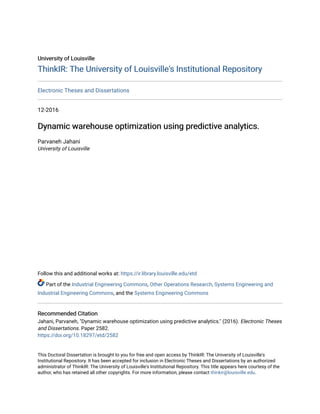
  • 49. Similar to Walter et al. (2013) study, we consider three product categories with a distribution D2. The probability of product belonging to category 1, 2, and 3 are .3, .4 and .3, respectively. We generate 100 independent instances for 33 = 27 experiments (three varying parameters P, S and pλ each with three choices). Four performance measures are: • ACI: Average percentage of cost improvement of G1 over DFRAAPES − R4. • ACD: Average percentage of cost difference between G1 and its continuous model counterpart. • SA: Same Assignment (but different allocation) in DFRAAPES − R4 and G1 via 100 replications. • SAA: Same Assignment and allocation in DFRAAPES − R4 and G1 via 100 replications. TABLE 2 Heuristics DFRAAPES − R4, G1 and continuous space model comparisons |P| = 12 |P| = 15 |P| = 18 P λ ACI ACD SA SAA ACI ACD SA SAA ACI ACD SA SAA r=1/3 0.2 0.12 2.15 83 74 0.13 2.07 69 68 0.10 1.99 66 65 0.5 0.18 2.90 76 69 0.17 3.04 70 70 0.07 2.82 82 82 0.8 6.84 0.21 100 58 0.00 3.74 100 100 0.16 4.29 84 80 r=1/2 0.2 0.22 2.12 65 64 0.28 2.29 54 54 0.11 2.72 61 61 0.5 0.63 2.59 56 51 0.40 3.01 68 65 0.16 3.93 71 71 0.8 2.21 0.15 100 58 6.13 0.73 38 16 2.56 0.90 100 64 r=2/3 0.2 0.78 2.18 60 54 0.44 2.23 54 52 0.30 2.88 48 46 0.5 1.42 2.57 79 68 2.99 2.55 66 42 1.57 3.04 39 33 0.8 1.38 0.11 100 42 0.86 0.33 100 74 3.28 0.29 100 18 32
  • 50. Table 2 lists the results of our computational study on the DFRAAPES − R4, G1, and continuous model. The numbers of this table represent the cost improvement of G1 over DFRAAPES − R4 or ACI is considerable for larger problems. The largest cost improvement (6.13%) happens for the moderate size of the forward area (r = 1/2), when P = 15. The assignment and allocation solutions of DFRAAPES −R4 and G1 are respectively similar in 38 and 16 out of 100 generated instances in this case. The assignment solutions of these two heuristics is more similar for lower additional costs resulted by picking more orders from the reserve area rather than the forward area (larger Pλ). As expected, the cost difference between G1 and its continuous counterpart becomes smaller for larger size forward areas. The adverse effect of the continuous model is more tangible for smaller forward area. Figure 9 confirms G1 outperforms DFRAAPES − R4 in all experiments. This figure also shows large probability of lower additional cost of picking from the re- serve area (large Pλ), specifically when the number is SKUs is low, results in smaller gap between G1 and its continuous counterpart. Note that our heuristics are based on greedy algorithm, while DFRAAPES − R4 is based on Bitran and Hax (1981) algorithm. Regarding the solution time, algorithm DFRAAPES − R4 applies Bitran and Hax (1981) algorithm with running time o(|p|2 ). Every generated combination set A ⊆ P (with at most o(2|p| ) running time) applies Bitran and Hax (1981) algorithm. Therefore, DFRAAPES −R4 solution time is o(|p|2 2|p| ) and it cannot be solved within reasonable time for large size problems. However, G1 delivers the assignment and allocation solution of P = 1000 in 10.42 seconds. In following, we address discrete assignment, allocation, and sizing problems together with no restriction on the width of SKUs that go into the forward area. 33
  • 51. 0 20 40 60 80 100 0 2 4 0 20 40 60 80 100 0 2 4 0 20 40 60 80 100 0 2 4 0 20 40 60 80 100 0 5 0 20 40 60 80 100 0 5 0 20 40 60 80 100 0 5 0 20 40 60 80 100 0 10 20 0 20 40 60 80 100 0 5 10 0 20 40 60 80 100 0 5 10 0 20 40 60 80 100 0 2 4 0 20 40 60 80 100 0 5 0 20 40 60 80 100 0 5 0 20 40 60 80 100 0 5 0 20 40 60 80 100 0 5 10 0 20 40 60 80 100 0 5 10 0 20 40 60 80 100 0 5 10 0 20 40 60 80 100 0 10 20 0 20 40 60 80 100 0 10 20 0 20 40 60 80 100 0 5 10 0 20 40 60 80 100 0 5 10 0 20 40 60 80 100 0 5 10 0 20 40 60 80 100 0 10 20 0 20 40 60 80 100 0 10 20 0 20 40 60 80 100 0 10 20 0 20 40 60 80 100 0 2 4 0 20 40 60 80 100 0 5 10 0 20 40 60 80 100 0 5 10 r=1/3 p λ =.8 r=1/2 pλ =.2 r=2/3 p λ =.8 r=1/2 pλ =.5 r=1/2 p λ =.8 r=2/3 pλ =.2 r=2/3 pλ =.5 r=1/3 p λ =.5 |P|=15 |P|=18 r=1/3 pλ =.2 |P|=12 Figure 9. The sorted ACI and ACD for 100 replications 34
  • 52. 3 Heuristic G2 Before explaining the heuristic G2, we represent the parameters used in the remainder of this chapter as following. Notation: 1. Rack information: W: Slot width L: Slot Depth H: Slot height O: Volume of slot (= WLH) NSL : Number of slots per shelf WSH : Shelf width NSH : Number of shelves per bay NB : Number of bays S: Total number of slots V : The volume of forward area (= NB NSH WSH LH) 2. SKU information: wi: Case width for SKU i li: Case length for SKU i hi: Case height for SKU i oi: Volume of carton of SKU i (= wilihi) bi: Eaches per case for SKU i di: Demand for SKU i per year pi: No. of picks for SKU i per year fi: Flow of SKU i in ft3 per year ϕi: Maximum possible stack for SKU i in slot (= l H hi m ). 35
  • 53. θi: Maximum possible No. of cartons of SKU i in depth of slot (= l L li m ). Input data: Rack information, SKU information, as above. Result: Optimally slotted SKUs into the carton flow rack (determines which SKUs should be stored in the forward area and number of slots given to SKU i, ni, in the forward area). Two important questions come up in discrete assignment-allocation problem with greedy algorithm perspective: 1. How to rank the SKUs in the discrete problem? 2. How many slots are given to the set of A ⊆ P SKUs selected for the forward area? The answer of these two questions in the continuous fluid model were addressed before. However, we need to apply a different approach for the discrete problem because of SKU and slot dimensions considerations and the resulted lost space. As previously defined, the flow rate of SKU i (fi) is the demand of SKU i per year translated to the volume per year. We need to revise the concept of flow in the discrete version of forward reserve problem to account for unavoidable wasted empty space due to the case(s) not completely occupying the slot(s) (see Figure 10). The practical flow fp i is: fp i = Number of slots required for SKU i per year × slot volume 36
  • 54. Therefore: fp i = & fi (ϕihi)(θili)W ' O (27) =     di bi oi (ϕihi)(θili)W     O (28) =     di bi wilihi (ϕihi)(θili)W     O (29) =     di bi wi ϕiθiW     O (30) Figure 10. The unavoidable wasted empty space due to the difference between the cases and the allocated slots dimensions. Example. Assume that the demand of SKU i per year is 320 units (eaches) and each case (carton) of SKU i has the capacity of 80 eaches (di = 320 and bi = 80). 37
  • 55. The dimension of the case for SKU i is: wi = 5 ft, li = 4 ft, hi = 4 ft. oi = wilihi = 80ft3 In the continuous model, where the slot dimensions are ignored, the flow of SKU i is equal to: fi = di bi oi = 320 80 80 = 320ft3 /year However, the slots’ dimensions are considered in discrete model. Assume: W = 6 ft, L = 6 ft, H = 10 ft O = WLH = 360 Practical flow fp i in discrete model is: fp i =     di bi wi ϕθW     O (31) = & (320 80 )5 (2)(1)(6) ' 360 (32) = 720ft3 /year (33) The difference between fi and fp i (400 ft3 ), is the volume of empty space around the cases stored in two slots of the forward area as shown in Figure 10. If we generalize this wasted space to all slots in forward area, the amount of lost space by discretizing the problem is non-trivial. The heuristic will inherently tend to reduce the lost space as much as possible. Consequently, we introduce parameter e in our heuristics in order not to exceed the capacity of the forward area and generate feasible solutions. As mentioned, only a fraction of the forward area space can be practically allocated to SKUs and the rest is wasted. This fraction depends on the selected set of SKUs for the forward area. So we search the best solution by examining different amounts of e in the range 0 < e ≤ 1. Finally, the best coefficient of space is found. We develop four procedures for ranking and fraction searching. yi in heuristic 38
  • 56. G2 is used for calculating the number of slots allocated to SKU i ni and is corresponded to the optimal space allocation in fluid model. For the first two procedures, where the SKU flows fis are cubic feet per year, yis are equal to the optimal cubic space given to SKU i in fluid model. However, the yis in the last two procedures are based on case movements per year. q0 i is the aggregate number of restocks of SKU i for the planning horizon period, if only a single slot (or minimum number of feasible slots for wi > W) is allocated to SKU i (q0 i = di biai .) ai is the units of SKU i that can be stored in minimum number of feasible slots allocated to the SKU and is defined as: ai =        θϕbW wi c if wi ≤ W θϕ otherwise The procedures are: A1: f1 i = di bi oi le1i = pi √ f1i y1 i = √ f1i P j∈A √ f1j S A2: f2 i = di bi oi le2i = pi √ fp i y2 i = √ f2i P j∈A √ f2j S A3: f3 i = di bi lei = pi √ f3i y3 i = √ f3i P j∈A √ f3j S A4: f4 i = di bi lei = pi √ f4i y4 i = √ q0 i P j∈A √ q0 j S While A1 and A2 rank the SKUs based on cubic feet movement of SKU, A3 and A4 use the number of cases needed during the planning horizon, instead of volume, for ranking SKUs. Note that the fraction given to SKU i in A4 corresponds to parameter q0 i, not fi. Of the four procedures, only A2 uses the practical flow fp i for labor efficiency computation. Heuristic G2 is a greedy algorithm based on rounding up the continuous model solution. After discretizing the non-integral solution, it applies a post processing 39
  • 57. step, called bottom-up deletion, for removing undesirable SKUs from the forward area. After assignment of SKUs and allocation of slots, it sorts the SKUs in order of non-increasing total number of restocks. Then, it deletes the SKU with minimum number of restocks (say 1 restock), and allocates its space to the SKU in the forward area with maximum number of restocks. We call this method bottom-up deletion, since the bottom SKU in number of restocks ranking will be deleted and its slot is added to the upper SKU in the ranking. We iterate this procedure until achieving no cost improvements. Heuristic G2 is as follow: 1. Rank all SKUs in order of non-increasing lei (different definitions for lei will be discussed) for i=1:No. of SKUs(N) do 2. Define n1i = wi W n2i = eyi O ni = max(n1i, n2i) 3. Get the assignment and allocation solutions and number of restocks (ri) end for 4. Rank all elements of SKUs assignment solution given by step (4) in order of non-increasing ri. 5. Apply bottom-up deletion approach: for j=1:No. of selected SKUs for forward area do 7. Remove the SKU with minimum ri and add its slot to the SKU with maxi- mum ri end for 40
  • 58. 8. Repeat steps (1) to (7) for different 0 e ≤ 1 with interval .1 to choose the one gives the minimum cost. 0 100 200 300 400 500 600 700 0.9 0.95 1 1.05 1.1 1.15 1.2 1.25 1.3 1.35 1.4 x 10 6 N o. of S KU s go i nto forward area To t a l co s t Figure 11. The cost reduction representation with increasing the number of SKUs in forward area. We consider a warehouse with 700 SKUs to determine the assignment, alloca- tion, and size of the forward area. The SKUs’ dimension data belongs to a real world warehouse. The best size of the forward area as suggested by G2 is 626 slots with 590 SKUs (see Figure 11). The minimum cost in Figure 11 occurs when to start adding those SKUs to the forward area that could be picked more efficiently from the reserve area. However, we have only 400 slots available in the forward area. Before applying the bottom-up deletion approach, the set of 374 SKUs leads 41
  • 59. 0 20 40 60 80 100 120 140 160 180 200 0.97 0.98 0.99 1 1.01 1.02 1.03 1.04 1.05 1.06 x 10 6 N o. of S KU rem oved from forward area i n b ottom -u p d el eti on ap p roach To t a l co s t Figure 12. The bottom-up deletion approach. to minimum cost of picking and replenishment. As Figure 12 shows, the bottom-up deletion approach in heuristic G2 recommends deleting 69 out of 374 SKUs from the forward area to devote their slots to those SKUs of the forward area with a higher number of restocks. The bottom-up deletion approach motivates having the uniform number of restocks among SKUs because the SKUs, which have had high number of restocks, no longer be replenished very frequently. Using this approach, they have more slots and more cases in the forward area because of allocating the slots of the deleted SKUs to them. The cost increment in iteration 52 of Figure 12 is associated with the situation, where the bottom-up deletion approach deletes one SKU with one slot from the forward area, but the candidate SKU for this slot from top of the list, needs more than one slot to be able to have one more lane in the forward area (wider SKU than slot width.) Therefore, we have one deleted SKU from the forward area 42
  • 60. without any value added and the total cost slightly increases. In our example, this approach reduces the total cost by 4.4%. D Comparisons We apply a data set from a telecommunications provider warehouse studied in Bartholdi and Hackman (2008) to compare the procedures. The warehouse that we addressed in our numerical example has 3049 SKUs, 30 bays, each having four shelves. In this warehouse, each shelf has eight equal standard size slots and therefore 960 slots. The algorithm suggested the best coefficient of space for this warehouse e = 0.17. Table 4 compares the costs of G2 for different procedures A1 to A4. The costs of A1, A3 and A4 are very close. However, A4 outperforms others in this example. TABLE 4 Cost comparisons between the procedures A1 to A4 using heuristic G2 A1 A2 A3 A4 No. of SKUs in forward area 805 783 721 722 Total cost 16237323 17035435 16190930 16182930 Solution time (seconds) 2.321091 1.903433 2.083014 2.123233 Cost Imp. of G2-A4 (%) 0.334988 5.004304 0.049408 - Using the same data set, Figure 13 shows the total cost of picking and restock- ing for heuristic G2 using A1 to A4. In this figure, the horizontal axis shows iteration i, when we add an SKU into the forward area in each step. We avoid naming this axis “Number of SKUs that go into the forward area,” since some SKUs selected for the forward area were removed in bottom-up deletion approach in heuristic G2. Figure 13 confirms the result of table 4 regarding the minimum cost of G2 using A4 scenario. 43
  • 61. The cost associated with G2 − A4 lies below the others. Using Figure 13, we can find the iteration that leads to the minimum cost, and then the best size of the forward area corresponding to that iteration can be obtained for each scenario. This figure provides practitioners a hint to decide about the size of forward area. 0 500 1000 1500 2000 2500 3000 3500 1.4 1.6 1.8 2 2.2 2.4 2.6 x 10 7 Iteration i Total cost G2−A3 G2−A4 G2−A1 G2−A2 Figure 13. The cost comparisons of G2 using different scenarios A1 to A4. In a second numerical example, we apply heuristic G2 −A1 to a real data set to compare the capability of the offered heuristics in assignment, allocation, and sizing of forward area with an available online software (http://www.warehouse-science.com/) by Bartholdi. In this example, the warehouse has 6498 SKUs and the slots of the for- ward area are assumed to be identical with given dimensions. The SKUs’ dimensions, demands, and picks data are given. The total cost is: 44
  • 62. X i∈P ni X j=1 (c1ipi + ci di aij )xij + X i∈P (c2ipi)xi0. (34) 0 1000 2000 3000 4000 5000 6000 7000 5.5 6 6.5 7 7.5 8 x 10 6 No. of SKU in the forward area Total cost Figure 14. Heuristic G2 − A1 for real world data set with 6498 SKUs. TABLE 5 Comparison of two methodologies for the discrete forward-reserve problem No. of SKUs in FW area No. of used slots Cost No. of replens. G2 − A1 4294 4318 5618853 3779 As observed in Figure 14 and Table 5, the optimal size of the forward area is 4318 slots. Giving more slots to the SKUs selected for the forward area than their allocated slots does not reduce their number of replenishment. So, the algorithm suggests to leave some slots unfilled. 45
  • 63. As Figure 14 shows, the total cost starts to increase after the minimum point of the curve because the algorithm assigns the SKUs with the low rank labor efficiency to the forward area. These SKUs can be picked more efficiently from the reserve area. According to the results, if we assign more than 4294 SKUs to the forward area, the total cost will grow due to the increase of replenishments. The solution time for G2 − A1 is 2.83 seconds. E Conclusion Unlike previous studies conducted on the forward reserve problem, which con- sider the continuous space of the forward area, we addressed the assigning and al- location of the discrete units of SKUs to their discrete slots. The gap between the continuous space model and its discrete counterpart has been quantified for different test problems. Our numerical results showed that the cost difference between the heuristic and its continuous counterpart decreases for larger size forward areas. First, we investigated the assignment, allocation, and the sizing problems si- multaneously. We determined the optimal size of the forward area while deciding the optimal set of SKUs for the forward area. Second, the proposed heuristics delivered a solution in seconds for the large size discrete forward-reserve problem with thousands of SKUs. Finally, we relaxed the assumption of assigning the SKUs to the shelves versus the slots, since this hypothesis limits the problem to the condition whereby the width of the opening is always greater than the SKU width. In all of the experiments, the cost comparison results showed that G1 always outperforms DFRAAPES −R4 in terms of the total cost of picking and replenishment. This cost improvement will become greater for larger size problems. While G1 works for the situations where the case and slot dimensions are not 46
  • 64. available, G2 considers these dimensions. The last two procedures for ranking the SKUs in the greedy algorithm, A3 and A4, which involve the discrete fi, outperform the first two procedures, A1 and A2, which contain a portion of the forward area’s continuous space, oi. Procedure A4 outperforms other procedures. It allocates the slots based on the aggregate number of restocks, if only a single (or minimum feasible number of slots) is allocated. 47
  • 65. CHAPTER III THE AREA SIZING AND SLOTTING OF A MULTI-MODE FORWARD AREA The picking and replenishment costs of the SKUs selected for the forward area can be reduced in multi-mode forward areas. While the number of cases stored in some pick modes can be more flexible, others have a fixed storage capacity. For example, the number of slots given to the SKUs in the carton flow rack are optimized by the allocation problem. The allocated slots can be one or multiple slots. However, the SKUs selected to be picked from the pallet flow rack are stored by a definite number of cases in the pallet. Different pick modes result in different number of replenishments for the SKUs selected for the forward area. Selecting the best types of racks (e.g. pallet flow rack, carton flow rack, bin shelving, etc.) and their effective size along with the best assignment of the SKUs to the pick mode within the forward area, considerably affects the total picking and replenishment cost. For instance, although pallet flow racks can hold many cases of an SKU on one pallet, a small quantity of that SKU can fit in one bin of bin shelving. As a result, the former has lower replenishment costs, but higher picking costs because of the lower pick density of items. On the other hand, the latter has lower picking cost inside the bay, but higher number of replenishments because of the smaller allocated space. After finding the best SKU assignment and slot allocation for each pick mode, the best size of the mode and so the overall size of the forward area are found. 48
  • 66. The classic Forward-Reserve Problem selects the best set of SKUs for the fast picking area of the warehouse and allocates the best number of slots to them having the size of the forward area. However, we will address the problem of determining the best number of bays/slots for each pick mode (e.g. pallet flow rack, carton flow rack, bin shelving, etc.) within the forward area, and we do so while determining the best SKU assignment and slot allocation. Considering an available space, we develop an algorithm, namely Profiling and Slotting Optimization (PSO) algorithm, which can increment number of bays of each pick mode, until adding more bays in the forward area increases the travel distance and costs (see Appendix.) Although expanding the forward area decreases the total number of replen- ishments, the large forward area has larger fixed picking and replenishment costs because of larger travel distance. Determining the best size of each pick mode, we calculate the cost of every possible combination of bays quantities corresponding to each pick mode, while not exceeding the available space. In each iteration, the best SKU assignment and slot allocation are found as well. In this chapter, one iteration of the PSO algorithm refers to generating one alternative for the forward area. The alternatives differ in their number of bays of each pick mode. The average travel distance for picking or replenishing of the items depends on the size of the pick mode. The average travel distance of a pick mode refers to the average horizontal distance that the labor traverses to pick or replenish an item (average aisle width) plus the average vertical distance (average aisle length). Therefore, our model accounts for the different picking and replenishment costs be- tween the pick modes with different sizes within an alternative and also between the same pick mode of different alternatives. The sequence of the pick modes within the forward area is assumed known and is taken into consideration while calculating the 49
  • 67. average travel distance. Therefore, the farther pick modes to the Input/Output point have higher average pick/replenishment travel distance(See Figure 15.) Figure 15. The multi-mode forward area Besides the travel distance analysis, SKU (each), case and slot dimensions are taken into consideration in the proposed model to conduct the fitting test for the replenishment unit and the slot. Furthermore, the model suggests the best orientation of replenishment unit (case), which enhances space utilization. The space allocation to the SKUs is discrete, as opposed to the traditional method of allocating continuous space to the SKUs. Jernigan (2004) develops a multi-tier inventory system. A multi-tier inventory system is an extension of the forward-reserve system with multiple forward modes. As opposed to our problem, which assumes all pick modes are replenished from the bulk storage, Jernigan (2004) establishes intermediate modes between the forward modes and the reserve area to reduce the restocking cost. The slotting of the inventory system in her study refers to finding the SKU assignment of the forward modes and the space allotted to the SKUs there, aiming to reduce the total picking and replenishment 50
  • 68. costs. While the volumes of the storage modes are known in Jernigan (2004)’s study, we optimize the size of the pick modes coupled with the slotting of the modes. Her study is also based on continuous space allocation, while we allocate discrete cases to the discrete number of slots slots, considering SKU and slot dimensions. The PSO algorithm, which can be found in appendix, accounts for: 1. Discrete case quantity movement: The small size fast movers have a low cubic feet movements. The continuous space allocation has the risk of assigning the small size fast movers to the high cost areas within the forward area and large size slow movers to the low cost areas within the forward area. Algorithm PSO is based on discrete quantity of moves for each SKU. 2. Discrete space allocation: PSO is a discrete space allocation model, which considers the lost spaces resulted from differences in slots and SKUs dimensions. Solving the allocation problem in a continuous space model causes many SKUs to have allocated space of less than the volume of one slot, which is impractical. Rounding up the solution and allocating one slot to these category leads to exceed the size of the forward area, which is infeasible. The PSO algorithm considers discrete space allocation, as opposed to the continuous space allocation of the picking areas. So, discrete units of the SKUs (case quantities) are stored in discrete units of slots. This concept prevents allocating a portion of a slot to the SKUs. 3. Replenishment unit fit test: If we do not check the dimensional fitness of the SKU to the slots of the pick modes, there is the risk of assigning the large size items in small size rack types. The PSO algorithm will consider both SKU and slot dimensions. 51
  • 69. 4. Optimizing case orientation: Finding the best case orientation in the rack and maximum feasible stack level leads to better space allocation and so more cases can be replenished in the slot. So, the number of replenishments will be reduced. SKU rotation allows the SKUs to have more options for being assigned to the different pick modes. The PSO suggests the best case orientation. Notation: 1. Rack information: j: Pick modes, j ∈ {0, 1, 2, 3} Wj: Slot width in pick mode j Lj: Slot Depth in pick mode j Hj: Slot height in pick mode j Oj: Volume of slot in pick mode j (= WjLjHj) NSH j : Number of shelves per bay in pick mode j NSL j : Number of slots per shelf in pick mode j NB j : Number of bays in pick mode j WSH j : Shelf width in pick mode j Vj: The volume of the pick mode j (= NB j NSH j WSH j LjHj) 2. SKU information: wsku i : Width of SKU i lsku i : Length of SKU i hsku i : Height of SKU i wi: Case width for SKU i li: Case length for SKU i hi: Case height for SKU i oi: Volume of case containing SKU i (= wilihi) bi: Eaches per case for SKU i 52
  • 70. Li: Find the number of lanes for SKU i in carton flow rack θij: Maximum No. of cases of SKU i in depth of slot in mode j(= l Lj li m ). ϕij: Maximum calculated stack level for SKU i in slot of mode j (= min(ρi, l Hj hi m ). ρi: Max given stack level of SKU i 3. Costs notation: cp j : Average picking cost from pick mode j. cr j: Average replenishment cost of pick mode j 0 (cr i0 = 0.) rij: Number of replenishments if SKU i is assigned to mode j 0 (ri0 = 0.) Cp ij: Picking cost if SKU i is assigned to mode j. Cr ij: Replenishment cost if SKU i is assigned to mode j 0 (Cr i0 = 0.) CT ij: Total picking and replenishment costs, if SKU i is picked from the mode j. sij: Saving of SKU i, if it is picked from mode j 0 rather than mode 0. The steps of the proposed algorithm for Profiling and Slotting Optimization of the forward area are as follow. The algorithm has been coded with the Python programming language. 1. Import data: Four types of data are imported: SKU data, order data, rack data and facility data. The SKU data provides the information about the case and SKU (each) dimension. The order file contains the historical demand data. The rack information delivers the setting of the racks in different types of pick modes (see table 10). The available space for designing the forward area and number of bays in the reserve area are provided by the facility data to estimate the fixed picking and replenishment costs. Table 7 summarizes the inputs parameters. 53
  • 71. TABLE 7 Inputs SKU Data Order Data Rack Data Facility Data SKU Number Time Width of a shelf Horizontal length of the forward area SKU Length SKU Number Depth of a shelf Vertical length of the forward area SKU Width Order quantity Height of a shelf No. of bays in one aisle of the reserve area SKU Height No. of level No. of aisles in reserve area Case Length No. of Slots per Shelf Case Width Case Height Case Pack Max Stack Level We assume that the pallet flow rack, which is generally the best option for the fast movers, is closest zone to the Pick up and Deposit (PD) point. Next, the carton flow rack and the bin shelving zones are designed (see Figure 15). We also consider three types of pick mode in our example warehouse. 2. Fit test: Based on SKU and slots dimensions, the SKUs that are not fitted to a particular type of slot will not be assigned to that rack type. 3. Case orientation: For all SKUs, the best case orientation in each pick mode that gives the maximum space utilization is determined in this section of the PSO algorithm. 4. Finding other parameters: The SKU demand di and picks pi, which is the sum of order quantity and the order lines per SKU during the planning horizon, respectively, and the SKU flow fi or the number of cases of SKU i during the planning horizon, are found in this step. fi can be found as: fi = di bi (35) 54
  • 72. We define aij as the number of cases of SKU i that can be stored in one pallet of a pallet flow rack (j = 1), the number of cases can be stored in minimum number of feasible slots in a carton flow rack (j=2), or one for bin shelving (j = 3). Assuming that the case pack quantity can fit in one bin of bin shelving, aij is obtained from: aij =        θijϕij j Wj wi k , if wi ≤ Wj θijϕij, otherwise. For the pallet flow rack, aij is calculated from the first equation of aij, because the case width is always less than the pallet width. For bin shelving, aij is one case. TABLE 8 6 possible case orientations in slot Orientation Wj Lj Hj 1 wij lij hij 2 wij hij lij 3 lij hij wij 4 lij wij hij 5 hij lij wij 6 hij wij lij For each SKU, we check 6 possible case orientations to find the best orientation of the case in pick mode j that gives the maximum aij (see Table 8.) We define q0 ij as the number of replenishments if the minimum number of slot(s) of mode j is allocated to the SKU and is calculated as below: q0 ij = fi aij (36) 55
  • 73. 5. Cost analysis: In this section, for every possible combination of the number of bays in each pallet flow rack, carton flow rack and bin shelving, the savings of picking from these areas versus picking from the reserve area are calculated for all SKUs. The slow movers with negative savings, however, are picked from the reserve area. The reserve area, pallet flow rack, carton flow rack, and bin shelving have the modes 0, 1, 2, and 3, respectively, in our example. To calculate the average picking and replenishment costs, we assume that the maximum horizontal length and vertical length of the available space for the forward area are given. The total costs and savings of an SKU by picking from the mode j are calculated as: rij = di mij ' (37) CT ij =Cp ij + Cr ij (38) =cp j pi + cr jrij (39) sij =CT i0 − CT i,j0, (40) where rij is the number of replenishment of SKU i in mode j. mij is the units (eaches) of SKU i in mode j. The algorithm for finding mij can be found in Appendix. 6. Export file: The algorithm will be terminated by exporting the outputs. We have implemented the PSO algorithm for an example warehouse with 28 SKUs. The rack information data can be found in Table 10. Using PSO algorithm, the optimal number of bays of pallet flow racks, carton flow racks and bin shelving, are 56
  • 74. TABLE 9 Outputs Slotting and Cost Data Size of each pick mode SKU No. Slots in CF No. bays of carton flow rack Pick mode Cases in CF No. bays of pallet flow rack Adjusted Width Lanes in CF No. of bays of bin shelving Adjusted Length Stacks in CF Adjusted Height Depth in CF Each fit CF? Ordered QTY Case fit CF? Order Lines Each fit PF? SKU Flow Case fit PF? Saving Each fit SH? Picking Cost Case fit SH? Replenishment Cost Total Cost PF = Pallet flow rack CF = Carton flow rack SH = Bin shelving 57
  • 75. 3,3,1, respectively ([NB 1 , NB 2 , NB 3 ]=[3,3,1].) If we expand the forward area more, the picking and replenishment costs will increase. The algorithm then suggests the best number of bays of each pick mode, along with the maximum total savings. TABLE 10 Rack information Carton Flow Rack (CF) Pallet Flow Rack (PF) Bin Shelving (SH) Width of a shelf 96 Width of a shelf 96 Width of a shelf 48 Depth of a shelf 96 Depth of a shelf 48 Depth of a shelf 21 Height of a shelf 20 Height of a shelf 60 Height of a shelf 12 Number of levels 4 Number of levels 1 Number of levels 5 Number of slots per Shelf 6 Number of slots per Shelf 2 Number of bins per shelf 4 1 Extensions The PSO algorithm (see Appendix) is a general model for sizing and slotting of the forward area’s zones. Considering the broad spectrum of requirements in real world warehouses, we evaluate the opportunities to empower the PSO algorithm in many ways. The goal is to explore and validate multiple pick mode design options that meet the distribution center’s requirements. The main features that have been added to the model are as follows: Volume growth and SKU growth Two types of growth affect the decisions made about the forward area: SKU growth and units growth. They should be considered while planning for the size of the pick modes. The units growth is the total growth in shipping units during the planning horizon, which includes the SKU growth as well. If no new SKU is introduced 58