Calculus in your nuts

1. HCMUT – DEPARTMEND OF MATH. APPLIED
---------------------------------------------------------------------------------------------------------------------
CALCULUS FOR BUSINESS – 221 Semester
CHAPTER 3: DERIVATIVE
• PhD. NGUYỄN QUỐC LÂN (November 2022)

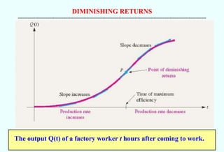
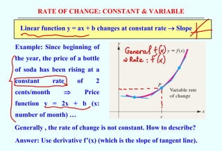
2. RATE OF CHANGE: CONSTANT & VARIABLE
--------------------------------------------------------------------------------------------------------------------------------------------
Linear function y = ax + b changes at constant rate → Slope
Example: Since beginning of
the year, the price of a bottle
of soda has been rising at a
constant rate of 2
cents/month  Price
function y = 2x + b (x:
number of month) …
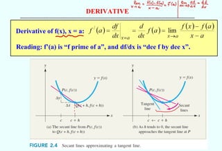
Generally , the rate of change is not constant. How to describe?
Answer: Use derivative f’(x) (which is the slope of tangent line).
- F
General + (x)
=> Rate = f(x)
=
S -
-------

3. PRACTICAL EXAMPLE
------------------------------------------------------------------------------------------------------------------------------------------------------------
----------------------------------------------------------------

4. DERIVATIVE
-----------------------------------------------------------------------------------------------------------------------------------
Derivative of f(x), x = a:
Reading: f’(a) is “f prime of a”, and df/dx is “dee f by dee x”.
=
(a)
-
! I

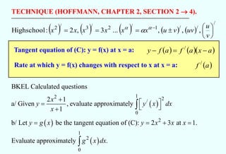
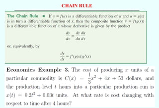
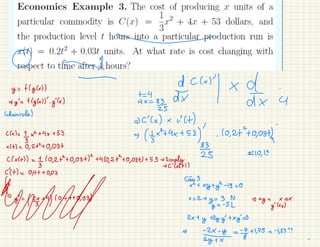
5. TECHNIQUE (HOFFMANN, CHAPTER 2, SECTION 2 → 4).
-----------------------------------------------------------------------------------------------------------------------------------
( ) ( ) ( ) ( ) ( )
/
/
/
1
/
2
/
3
/
2
,
,
,
...
3
,
2
:
Highschool 






=
=
= −
v
u
uv
v
u
x
x
x
x
x
x 


Tangent equation of (C): y = f(x) at x = a:
Rate at which y = f(x) changes with respect to x at x = a:
( ) ( )( )
a
x
a
f
a
f
y −
=
− /
( )
a
f /
( )
( )
( )
1
2 2
/
0
2
1
2
0
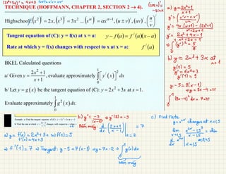
BKEL Calculated questions
2 1
a/ Given , evaluate approximately
1
b/ Let be the tangent equation of (C): 2 3 at 1.
Evaluate approximately .
x
y y x dx
x
y g x y x x x
g x dx
+  
=
 
+
= = + =



6. 12x+
3x)' = 4x+ 3 (or)= vv + uv
(cost)=
-
sinx
a) y=
x+ 1
↑
j =
/
y =
I
5
b)
y
= 2x
3
+ 3x at
x = 1
y(1) = 5
y = 6x2+ 3
y'(1) = 9
y
- 5 = 9(x -
1)
=>
y
= gx -
4 = 1 !
S 19x -
4) 2dx = = = x)
b)y=
=
= y'(2) = -
3 c) Find Wate
(x -
1)2
y =
xXchanges at x = 1,
5
= 2
a)
y
=
f()=2+
3x = f() = 5
Bam may
:)k= 2
*
Eme
(x =
15
=9
,45
=> f ' (1) = 7 =>
Tangent:
y
-
5 = 7(x -
1) =
y
= 7x -
2
+(g(x)dx
·
may

7. RATE OF CHANGE
-----------------------------------------------------------------------------------------------------------------------------------
2 1
Example: Find the rate at which changes with respect to at 2
1
x
y x x
x
+
= =
−
Rate at which y = f(x) changes with respect to x at x = a: ( )
a
f /

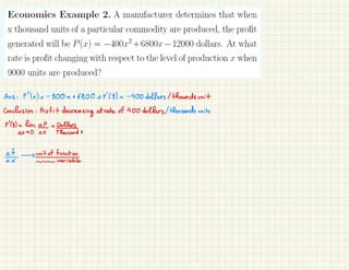
8. Ans : P'(x) =
-
800x + 6800 = 4'/9) =
-
400 dollars/thounds unit
Conclusion : Profit
decreasing atrate of 400 dollars/thousands units
p'(g)lim
Dollarsds
- >
unit of function
~
variable

9. CHAIN RULE
-----------------------------------------------------------------------------------------------------------------------------------

10. -
0 =
y =
f(g(x))
-
+= 4 dc() + d
= y= + (g(x))'-
g(x) = + = 8 dx4
25
Khainrutel
=> c'(x) + v()
,
((x)=
1x
+ 4x + 53
=>
(y*+ 4x +
53) ·
10,
2++ 0
,
037)
x( +) = 0,
2+
2
+ 0
,
037
3 = 10,
13
c(x(+) =
1(0,
2++ 0
,
03 +12 + 410,
2 +
2
+ 0
,
037) + 53- Simply
-
> C'(xk+ 1)
c'(+) = 0,
4 + + 0
,03
x+
xy+
y
-
-
19 = 0
10
,
4 + + 0, 03
Cau
y
= -
SL y'(x0)
x = 2 +
y
= 3N =
oy = XXX
2x +
y
+
2y y + xy=0
=>
-
2x -
y =
=
x,
75 +
-
1
,
53 ??
-
2y + x
-

11. MARGINAL ANALYSIS
--------------------------------------------------------------------------------------------------------------------------------------------
In economics, the use of the derivative to approximate the change
in a quantity that results from one (1) – unit increase in
production is called marginal analysis
Which argument could we use to try to buy one airticket for
Hochiminh City – Ha Noi in (for example!) 100k VND?

12. Remember :
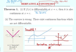
* fin f(x) = => When x = x
,
f(x)L En
x +
x0
x0 fk) =1
2
* f(a)
=lim
I
If +x = 1(00x = x
-
a =
1 = x = a + 1)
ingrits
on
=> f(a+h) -
f(a) = +'(a)(* )
= Whenx = 0
:
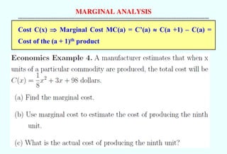
+(a) zotef(a). * Cost function :
Cale()
:
units "The change ofproduct
((9) (((9)
102unit
nd
-
(19) : The costof 10 unit

13. MARGINAL ANALYSIS
--------------------------------------------------------------------------------------------------------------------------------------------
Cost C(x)  Marginal Cost MC(a) = C’(a)  C(a +1) – C(a) =
Cost of the (a + 1)th product

14. -
change of cost
when x = a 1 unit
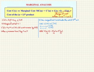
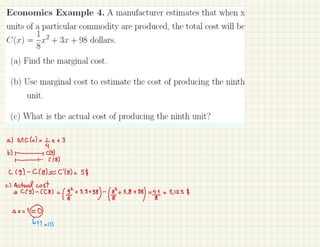
((x) =
292+
49 , 970 2) Use marginalcost to estimate the costof 15thun it
1) Marginal costat 4 ? ((is) -
((14) = C' (14)
C'(q) =
4q + 4 = C(4) = 20 = cost increase
by 20$ T
I-
15 14 14
When
a increase from4 by
T unit Nho f(a+ 1) -
f(a) = f'(a)

15. a) Mc(x) =
+x + 3
b) m ((9)
-
. . .
((8)
((9) -
C(8) =C'(8) = 59
c) Actual cost
= ((g) -
(28) =
( + 3.
9 +
98)-
(+ 3.
8 +
98) = = 5
, 12
-x =
10
- ?? = 1)

16. EXAMPLE
--------------------------------------------------------------------------------------------------------------------------------------------
A manufacturer of digital cameras estimates that when x hundred
cameras are produced, the total profit will be P(x) = –0.0035x3 +
0.07x2 + 25x – 200 thousand dollars.
(a) Find the marginal profit function
(b) What is the marginal profit when the level of production is x =
10, x = 50 and x = 80?
(c) Interpret these results.
Revenue R(x)  Mar. Reve. MR(a) = R’(a)  R(a + 1) – R(a)
Profit P(x)  Marginal Profit MP(a) = P’(a)  P(a + 1) – P(a)

17. #
M .
prote
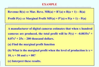
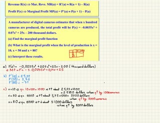
a P(x) =
-
0,
0035x3 + 0.
07x + 25x -
200/thousand dollars)
=> MP = P=
-
3 .
0,
0035x + 0
,
14x + 25
b) P' (10) = 25,
35
P(55 -
c) x = 10 =
) q
= 10x100 = 1000 = 44 about 25,
35x1000
= 25350 dollars when qt by 1000cameras
x = 50 = q = 5000 = PT about 5
,
75x1000 = 5750 dollars
when
↑ by 5000 cameras
x = 80 =
q = 8000 = 4t about 31000 dollars
When
qt by 8000 dollars

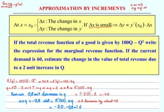
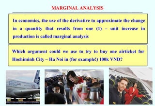
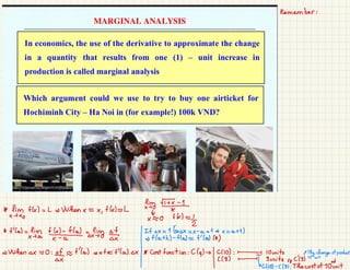
18. APPROXIMATION BY INCREMENTS
--------------------------------------------------------------------------------------------------------------------------------------------
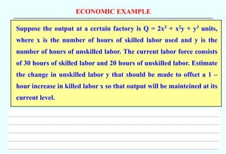
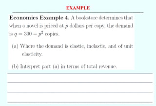
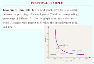
If the total revenue function of a good is given by 100Q – Q2 write
the expression for the marginal revenue function. If the current
demand is 60, estimate the change in the value of total revenue due
to a 2 unit increase in Q
( ) x
x
y
y
x
y
y
x
x
x
x 










= 0
/
0 small
is
If
.
in
change
The
:
in
change
The
:
:
At
himy => X 0
by zy-
0x
-
R(q) = 100Q -
Q = Mr =
R'(q) = 100 -
29
q
= 60 : 2 unit Y
ing =
q
= 2 = 0 RvR'(60) .
09
Remain O,
Susit decrease in
q
= (-
20) .
2 =
-
40
=>
rq
= - 0
.
8 =R = R160) .
q
= R decrease
by about 40
=
= 20 . -0
.
8 = 16

19. IMPLICIT FUNCTION
-----------------------------------------------------------------------------------------------------------------------------------
The functions we have met so far can be described by y = f(x)
Some functions, however, are defined implicitly by a relation between
x & y such as x^3 + y^3 = 6xy  y = y(x): Implicit function
An equation F(x, y) = 0 defines
implicitly one (or more)
function y = y(x):
F(x, y(x)) = 0
These functions are called
implicit function
x = 0 +
y3= 0
ycan' +3
* = 0
+
y3-
18y + 27
y
= 3
Zy
= =

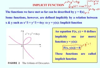
20. IMPLICIT DIFFERENTIATION
-----------------------------------------------------------------------------------------------------------------------------------
Method of Implicit Differentiation: Differentiating both sides of the
equation F(x, y) = 0 with respect to x, regarding always y = y(x), and
then solving the resulting equation for y’.
3)
(3;
at
6
:
(C)
curve
the
o
tangent t
the
Find
b/
6
if
Find
a/
:
Example
3
3
3
3
/
xy
y
x
xy
y
x
y
=
+
=
+
(x2)"= 2x
(02)' = 2u.
r
3y-
y
irongigtons
=> (x +yS)y= (Gxy)x
not
Cy
Look at
Hoffman
Implicit diff
xy + xy
a)3x2 +
3y .
y =
G[y +
xy] = (3y2-
(x)y =
by -
3x= y =
(2
-
x
y
--
2x
b) A
+ (3
,
3) :
y
=
=>
Tangent :
%0
↓
To
y
-
3 =
-
1(x -
3) =
y
=
-
x + 6

21. ECONOMIC EXAMPLE
---------------------------------------------------------------------------------------------------------------------------------------------------
Suppose the output at a certain factory is Q = 2x3 + x2y + y3 units,
where x is the number of hours of skilled labor used and y is the
number of hours of unskilled labor. The current labor force consists
of 30 hours of skilled labor and 20 hours of unskilled labor. Estimate
the change in unskilled labor y that should be made to offset a 1 –
hour increase in killed labor x so that output will be mainteined at its
current level.

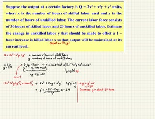
22. Output a =
f(x
, y)
Q = 2x +
xy +
y x : numbers of hours of skill labors
y
: numbers of hours of unskill labors
x = 30 x ↓
by thour -
> a = constant => 2x3 + x
y
+ y = const
y
= 20
& yt by how much
&
um
y
=
y(x) =
y
-y
=
y
- 0x
Xx = 1
(2x3 +
y +
y)) =
(const) = 6x2 +
2xy + x
y 3yy = 0
by
=
y. x
I
=
- 3
,
14
=>
y
=
eye-3
=>
Decrease
y in
about 3
,
14 hours

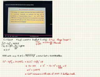
23. C =
C(q) unit F(c, q) = const -
> Implicit C =
Clq) If
g,
c
change /respect ?
[C
-
39 = 4275 Chaina
9 , 9 =
g(t)
, d
I
given
= C =?
1500 units =>
q = 15 = C =
27 = 120 Cost = 120000 dollars
(c
2
-
39)! = 142751+ + 2CC -
99q = 0
=> 2x120xc -
9x15x
=> c = 1
,
6875
=> Cost increases with rate of 1687 .
5 dollars /week.

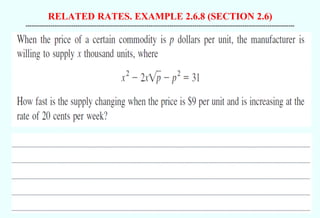
24. RELATED RATES. EXAMPLE 2.6.8 (SECTION 2.6)
--------------------------------------------------------------------------------------------------------------------------------------------

25. RELATED RATES. EXAMPLE 2
-----------------------------------------------------------------------------------------------------------------------------------

26. DERIVATIVE & CONTINUOUS
--------------------------------------------------------------------------------------------------------------------------------------------
lim
#im
+ (x) = +(c)
-
has derivative
Smooth ?
~
I #
-
>
Derivative => ContiniousC
#

27. EXAMPLE
--------------------------------------------------------------------------------------------------------------------------------------------
end answer
x + 0 ,
=
8 continuous ea=
flo)linting(x) =
1 =
g(0) =
+( =
g()vxref
6
First ,
a = f(0) = limf(x)
x - 0
e
! 1x
-
>0
=I =L
When a =
1+d
=

28. INCREASING – DECREASING FUNCTION (HOFFMANN, CH. 3)
--------------------------------------------------------------------------------------------------------------------------------------------

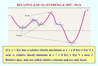
29. RELATIVE (LOCAL) EXTREMA & MIN - MAX
--------------------------------------------------------------------------------------------------------------------------------------------
(C): y = f(x) has a relative (local) maximum at x = c if f(c)  f(x)  x
near c; relative (local) mininum at x = c if f(c)  f(x)  x near c.
Relative max, min are called relative extrema and are only local.

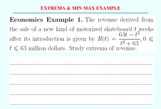
30. EXTREMA & MIN MAX EXAMPLE
--------------------------------------------------------------------------------------------------------------------------------------------

31. DIMINISHING RETURNS
--------------------------------------------------------------------------------------------------------------------------------------------
The output Q(t) of a factory worker t hours after coming to work.

32. INFLECTION POINTS
--------------------------------------------------------------------------------------------------------------------------------------------
An inflection point (or point of inflection) is a point (c, f(c))  (C): y
= f(x) where the concavity (that means f’’) changes. At such a point,
either f’’(c) = 0 or f’’(c) does not exist.
( ) .
7
5
2
poins
Inflection
:
Example
4
6
t
t
t
t
Q +
−
=

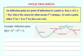
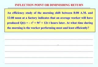
33. INFLECTION POINT OR DIMINISHING RETURN
--------------------------------------------------------------------------------------------------------------------------------------------
An efficiency study of the morning shift between 8:00 A.M. and
12:00 noon at a factory indicates that an average worker will have
produced Q(t) = – t3 + 9t2 + 12t t hours later. At what time during
the morning is the worker performing most and least efficiently?

34. (PRICE ELASTICITY OF DEMAND)
--------------------------------------------------------------------------------------------------------------------------------------------

35. EOD EXAMPLE
--------------------------------------------------------------------------------------------------------------------------------------------

36. CLASSIFICATION
--------------------------------------------------------------------------------------------------------------------------------------------

37. CLASSIFICATION AND REVENUE
--------------------------------------------------------------------------------------------------------------------------------------------

38. EXAMPLE
--------------------------------------------------------------------------------------------------------------------------------------------