© 2019 Cengage. All Rights Reserved. Linear RegressionC.docx

© 2019 Cengage. All Rights Reserved.
Linear Regression
Chapter 4
Introduction (Slide 1 of 2)
• Managerial decisions are often based on the relationship
between two or
more variables:
• Example: After considering the relationship between
advertising
expenditures and sales, a marketing manager might attempt to
predict sales
for a given level of advertising expenditures.
• Sometimes a manager will rely on intuition to judge how two
variables
are related.
• If data can be obtained, a statistical procedure called
regression analysis
can be used to develop an equation showing how the variables
are
related.

Introduction (Slide 2 of 2)
• Dependent variable or response: Variable being predicted.
• Independent variables or predictor variables: Variables being
used
to predict the value of the dependent variable.
• Simple linear regression: A regression analysis for which any
one
unit change in the independent variable, x, is assumed to result
in
the same change in the dependent variable, y.
• Multiple linear regression: A regression analysis involving
two or
more independent variables.
Simple Linear Regression Model
Regression Model
Estimated Regression Equation
Simple Linear Regression Model (Slide 1 of 5)
Regression Model:
• The equation that describes how y is related to x and an error

term.
• Parameters:
• The error term accounts for the variability in y that cannot be
explained by
the linear relationship between x and y.
Estimated Regression Equation:
• The parameter values are usually not known and must be
estimated using
sample data.
• Sample statistics 0 1(denoted and )b b are computed as
estimates of the
population parameters
• Substituting the values of the sample statistics 0 1 0 1 and for
the regression equation and dropping the error term, we obtain
the
estimated regression for simple linear regression.

• In the estimated simple linear regression equation:
0 1ŷ b b x= +
• ŷ = Estimate for the mean value of y corresponding to a given
value of x.
• 0b = Estimated y-intercept.
•
1b = Estimated slope.
• The graph of the estimated simple linear regression equation is
called the
estimated regression line.
• In general, ŷ is the point estimator of ( ) ,E y x the mean value
of y for a
given value of x.
Figure 7.1: The Estimation
Process in Simple Linear
Regression

Figure 7.2: Possible Regression Lines in Simple Linear
Regression
Least Squares Method
Least Squares Estimates of the Regression Parameters
Using Excel’s Chart Tools to Compute the Estimated Regression
Equation
Least Squares Method (Slide 1 of 15)
• Least squares method: A procedure for using sample data to
find
the estimated regression equation.
• Determine the values of 0 1 and .b b
• Interpretation of 0 1 and :b b
• The slope
1b is the estimated change in the mean of the dependent
variable y that is associated with a one unit increase in the
independent variable x.
• The y-intercept 0b is the estimated value of the dependent
variable y

when the independent variable x is equal to 0.
Table 7.1: Miles Traveled
and Travel Time for 10
Butler Trucking Company
Driving Assignments
Driving Assignment i x = Miles Traveled
y = Travel Time
(hours)
1 100 9.3
2 50 4.8
3 50 8.9
4 100 6.5
5 50 4.2
6 80 6.2
7 75 7.4
8 65 6.0
9 90 7.6

10 90 6.1
Figure 7.3: Scatter
Chart of Miles
Traveled and Travel
Time for Sample of
10 Butler Trucking
Company Driving
Assignments
• thi residual: The error made using the regression model to
estimate the
mean value of the dependent variable for the thi observation.
• Denoted as ˆ .i i ie y y= −
• Hence,
( )

2 2
1 1
ˆmin min
n n
i i i
i i
y y e
= =
• We are finding the regression that minimizes the sum of
squared
errors.
Least Squares Estimates of the Regression Parameters:
• For the Butler Trucking Company data in Table 7.1:
• Estimated slope of 1 0.0678.b =
• y-intercept of 0 1.2739.b =
• The estimated simple linear regression model:
1
ˆ 1.2739 0.0678y x= +

• Interpretation of 1:b If the length of a driving assignment were
1 unit
(1 mile) longer, the mean travel time for that driving assignment
would be 0.0678 units (0.0678 hours, or approximately 4
minutes)
longer.
• Interpretation of 0:b If the driving distance for a driving
assignment
was 0 units (0 miles), the mean travel time would be 1.2739
units
(1.2739 hours, or approximately 76 minutes).
• Experimental region: The range of values of the independent
variables in the data used to estimate the model.
• The regression model is valid only over this region.
• Extrapolation: Prediction of the value of the dependent
variable
outside the experimental region.
• It is risky.

• Butler Trucking Company example: Use the estimated model
and the
known values for miles traveled for a driving assignment (x) to
estimate
mean travel time in hours.
• For example, the first driving assignment in Table 7.1 has a
value for miles
traveled of 100.x =
• The mean travel time in hours for this driving assignment is
estimated to be:
( )1ˆ 1.2739 0.0678 100 8.0539y = + =
• The resulting residual of the estimate is:
1 1 1
ˆ 9.3 8.0539 1.2461e y y= − = − =
Table 7.2: Predicted Travel Time and Residuals for 10 Butler
Trucking
Company Driving Assignments

Figure 7.4: Scatter Chart of
Miles Traveled and Travel
Time for Butler Trucking
Company Driving
Assignments with
Regression Line
Superimposed
Figure 7.5: A Geometric
Interpretation of the
Least Squares Method
Using Excel’s Chart Tools to Compute the Estimated Regression
Equation:
• After constructing a scatter chart with Excel’s chart tools:
1. Right-click on any data point and select Add Trendline.
2. In the Format Trendline task pane, in the Trendline Options
area:
• Select Linear.

• Select Display Equation on chart.
Figure 7.6: Scatter
Chart and
Estimated
Regression Line
for Butler Trucking
Company
Slope Equation
( )( )
( )
1
1
2
1
n
i i
i

n
i
i
x x y y
b
x x
=
=
− −
=
−
y-Intercept Equation
0 1b y b x= −
value of the independent variable for the th observation.
value of the dependent variable for the th observation.
mean value for the independent variable.

mean value for the dependent var
i
i
x i
y i
x
y
=
=
=
= iable.
total number of observations.n =
Assessing the Fit of the Simple
Linear Regression Model
The Sums of Squares
The Coefficient of Determination
Using Excel’s Chart Tools to Compute the Coefficient of
Determination

Assessing the Fit of the Simple Linear
Regression Model (Slide 1 of 10)
The Sums of Squares:
• Sum of squares due to error: The value of SSE is a measure of
the error in using the
estimated regression equation to predict the values of the
dependent variable in the
sample.
From Table 7.2,
2
1
SSE 8.0288
n
i
i
e
=

Figure 7.7: The
Sample Mean y
as a Predictor of
Travel Time for
Butler Trucking
Company
• Table 7.3 shows the sum of squared deviations obtained by
using
the sample mean 6.7y = to predict the value of travel time in
hours
for each driving assignment in the sample.
• Butler Trucking Example: For the thi driving assignment in
the
sample, the difference iy y− provides a measure of the error
involved in using y to predict travel time for the thi driving
assignment.
• The corresponding sum of squares is called the total sum of
squares (SST).

Table 7.3:
Calculations for
the Sum of
Squares Total for
the Butler
Trucking Simple
Linear Regression
Figure 7.8:
Deviations About
the Estimated
Regression Line and
the Line y y=
for the Third Butler
Trucking Company
Driving Assignment

• Measures how much the ŷ values on the estimated regression
line deviate
from .y
• Relation between SST, SSR, and SSE:
SST = SSR + SSE
where
• SST = total sum of squares
• SSR = sum of squares due to regression
• SSE = sum of squares due to error.
The Coefficient of Determination:
• The ratio SSR/SST used to evaluate the goodness of fit for the
estimated
regression equation; this ratio is called the coefficient of
determination
and is denoted by 2.r
• Take values between zero and one.
• Interpreted as the percentage of the total sum of squares that
can be
explained by using the estimated regression equation.

Using Excel’s Chart Tools to Compute the Coefficient of
Determination:
• To compute the coefficient of determination using the scatter
chart in
Figure 7.3:
1. Right-click on any data point in the scatter chart and select
Add
Trendline.
2. When the Format Trendline task pane appears: Select Display
R-
squared value on chart in the Trendline Options area.
Figure 7.9: Scatter
Chart and Estimated
Regression Line with
Coefficient of
Determination 2r
for Butler Trucking
Company

The Multiple Regression Model
Regression Model
Estimated Multiple Regression Equation
Least Squares Method and Multiple Regression
Butler Trucking Company and Multiple Regression
Using Excel’s Regression Tool to Develop the Estimated
Multiple Regression Equation
The Multiple Regression Model (Slide 1 of 11)
Regression Model:
• y = dependent variable.
• 1 2, , . . ., qx x x = independent variables.
•
eters.
explained
by the linear effect of the q independent variables).
Regression Model (cont.):

•
in the mean
value of the dependent variable y that corresponds to a one unit
increase
in the independent variable ,jx holding the values of all other
independent variables in the model constant.
• The multiple regression equation that describes how the mean
value of y
is related to 1 2, , . . ., :qx x x
Estimated Multiple Regression Equation:
Least Squares Method and Multiple Regression:
• The least squares method is used to develop the estimated
multiple
regression equation:
• Finding ( )
2 2
0 1 2 1 1

ˆ, , , , that satisfy min min .
n n
q i i ii i
b b b b y y e
= =
• Uses sample data to provide the values of 0 1 2, , , , qb b b b
that minimize the
sum of squared residuals.
Figure 7:10: The
Estimation Process for
Multiple Regression
Butler Trucking Company and Multiple Regression:
• The estimated simple linear regression equation, ˆ 1.2739
0.0678 .i iy x= +
• The linear effect of the number of miles traveled explains
66.41%

( )2 0.6641r = of the variability in travel time in the sample
data.
• This implies, 33.59% of the variability in sample travel times
remains
unexplained
• The managers might want to consider adding one or more
independent
variables, such as number of deliveries, to the model to explain
some of
the remaining variability in the dependent variable.
Butler Trucking Company and Multiple Regression (cont.):
• Estimated multiple linear regression with two independent
variables:
0 1 1 2 2ŷ b b x b x= + +
• ŷ = Estimated mean travel time.
• 1x = Distance traveled.
• 2x = Number of deliveries.
• The SST, SSR, SSE and 2R are computed using the formulas
discussed
earlier.

Using Excel’s Regression Tool to Develop the Estimated
Multiple
Regression Equation:
Figure 7.11: Data Analysis Tools Box
Figure 7.12: Regression
Dialog Box
Figure 7.13: Excel Regression Output for the Butler Trucking
Company
with Miles and Deliveries as Independent Variables
Figure 7.14: Graph of
the Regression
Equation for Multiple
Regression Analysis

with Two
Independent
Variables
Inference and Regression
Conditions Necessary for Valid Inference in the Least Squares
Regression Model
Testing Individual Regression Parameters
Addressing Nonsignificant Independent Variables
Multicollinearity
Inference and Regression (Slide 1 of 15)
• Statistical inference: Process of making estimates and drawing
conclusions about one or more characteristics of a population
(the value
of one or more parameters) through the analysis of sample data
drawn
from the population.
• In regression, inference is commonly used to estimate and
draw
conclusions about:

• The mean value and/or the predicted value of the dependent
variable y for
specific values of the independent variables * * *1 2, , , .qx x x
• Consider both hypothesis testing and interval estimation.
Conditions Necessary for Valid Inference in the Least Squares
Regression Model:
• For any given combination of values of the independent
variables
normally
distributed with a mean of 0 and a constant variance.
Figure 7.15: Illustration of
the Conditions for Valid
Inference in Regression

Figure 7.16: Example of a Random Error Pattern in a Scatter
Chart of
Residuals and Predicted Values of the Dependent Variable
Figure 7.17: Examples of
Diagnostic Scatter Charts
of Residuals from Four
Regressions
Figure 7.18: Excel Residual Plots for the Butler Trucking
Company
Multiple Regression
Figure 7.19: Table of the
First Several Predicted
Values ŷ and Residuals e
Generated by the Excel
Regression Tool

Figure 7.20: Scatter
Chart of Predicted
Values ŷ and
Residuals e
Testing Individual Regression Parameters:
• To determine whether statistically significant relationships
exist between
the dependent variable y and each of the independent variables
1 2, , , qx x x individually.
dependent variable y
and the independent variable .jx
Testing Individual Regression Parameters (cont.):

• Use a t test to test the hypothesis that a regression parameter
is zero.
• The test statistic for this t test, .
j
j
b
b
t
s
=
jb
s = Estimated standard deviation of .jb
• As the magnitude of t increases (as t deviates from zero in
either
direction), we are more likely to reject the hypothesis that the
regression
Testing Individual Regression Parameters (cont.):
• Confidence interval can be used to test whether each of the
regression
parameters

• Confidence interval: An estimate of a population parameter
that
provides an interval believed to contain the value of the
parameter at
some level of confidence.
• Confidence level: Indicates how frequently interval estimates
based on
samples of the same size taken from the same population using
identical
sampling techniques will contain the true value of the parameter
we are
estimating.
Addressing Nonsignificant Independent Variables:
• If practical experience dictates that the nonsignificant
independent
variable has a relationship with the dependent variable, the
independent
variable should be left in the model.
• If the model sufficiently explains the dependent variable
without the
nonsignificant independent variable, then consider rerunning the
regression without the nonsignificant independent variable.
• The appropriate treatment of the inclusion or exclusion of the

y-intercept
when 0b is not statistically significant may require special
consideration.
Multicollinearity:
• Multicollinearity refers to the correlation among the
independent
variables in multiple regression analysis.
• In t tests for the significance of individual parameters, the
difficulty
caused by multicollinearity is that it is possible to conclude that
a
parameter associated with one of the multicollinear independent
variables is not significantly different from zero when the
independent
variable actually has a strong relationship with the dependent
variable.
• This problem is avoided when there is little correlation among
the
independent variables.
Figure 7.21: Excel Regression Output for the Butler Trucking
Company

with Miles and Gasoline Consumption as Independent Variables
Chart of Miles and
Gasoline Consumed for
Butler Trucking
Company
Big Data and Regression (Slide 1 of 2)
Multicollinearity (cont.):
• Testing for an overall regression relationship:
• Use an F test based on the F probability distribution.
• If the F test leads us to reject the hypothesis that the values of
1 2, , , qb b b
are all zero:
• Conclude that there is an overall regression relationship.
• Otherwise, conclude that there is no overall regression
relationship.

Big Data and Regression (Slide 2 of 2)
Multicollinearity (cont.):
• Testing for an overall regression relationship (cont.):
• The test statistic generated by the sample data for this test is:
( )
SSR
SSE 1
q
F
n q
=
− −
• SSR = Sum of squares due to regression.
• SSE = Sum of squares due to error.
• q = the number of independent variables in the regression
model.
• n = the number of observations in the sample.
• Larger values of F provide stronger evidence of an overall
regression
relationship.
Categorical Independent

Variables
Butler Trucking Company and Rush Hour
Interpreting the Parameters
More Complex Categorical Variables
Categorical Independent Variables (Slide 1 of 10)
Butler Trucking Company and Rush Hour:
• Dependent variable, y: Travel time.
• Independent variables: miles traveled ( )1x and number of
deliveries ( )2 .x
• Categorical variable: rush hour ( )3x = 0 if an assignment did
not include
travel on the congested segment of highway during afternoon
rush hour.
• Categorical variable: rush hour ( )3x = 1 if an assignment
included travel
on the congested segment of highway during afternoon rush
hour.
Figure 7.23: Histograms of the Residuals for Driving
Assignments That

Included Travel on a Congested Segment of a Highway During
the Afternoon
Rush Hour and Residuals for Driving Assignments That Did Not
Figure 7.24: Excel
Data and Output for
Butler Trucking with
Miles Traveled 1( ),x
Number of Deliveries
2( ),x and the Highway
Rush Hour Dummy
Variable 3( ),x as the
Independent Variables
Interpreting the Parameters:
• The model estimates that travel time increases by:
• 0.0672 hours for every increase of 1 mile traveled, holding
constant the
number of deliveries and whether the driving assignment route
requires
the driver to travel on the congested segment of a highway
during the
afternoon rush hour period.

• 0.6735 hours for every delivery, holding constant the number
of miles
traveled and whether the driving assignment route requires the
driver to
travel on the congested segment of a highway during the
afternoon rush
hour period.
Interpreting the Parameters (cont.):
• The model estimates that travel time increases by (cont.):
• 0.9980 hours if the driving assignment route requires the
driver to travel on
the congested segment of a highway during the afternoon rush
hour period,
holding constant the number of miles traveled and the number
of
deliveries.
• 2 0.8838R = indicates that the regression model explains
approximately
88.4% of the variability in travel time for the driving
assignments in the
sample.

Interpreting the Parameters (cont.):
• Compare the regression model for the case when 3 0x = and
when
3 1.x =
• When
3 0:x =
• When 3 1:x =
More Complex Categorical Variables:
• If a categorical variable has k levels, 1k − dummy variables
are required,
with each dummy variable corresponding to one of the levels of
the
categorical variable and coded as 0 or 1.
• Example:
• Suppose a manufacturer of vending machines organized the
sales territories
for a particular state into three regions: A, B, and C.
• The managers want to use regression analysis to help predict
the number of
vending machines sold per week.
• Suppose the managers believe sales region is one of the

important factors
in predicting the number of units sold.
More Complex Categorical Variables (cont.):
• Example (cont.):
• Sales region: categorical variable with three levels (A, B, and
C).
• Number of dummy variables = 3 2 1.− =
• Each variable can be coded 0 or 1 as:
1 1 if sales Region B; 0 if otherwise.x =
2 1 if sales Region C; 0 if otherwise.x =
• The values of
1 2 and are:x x
• The regression equation relating the mean number of units
sold to the

dummy variables is written as:
0 1 1 2 2ŷ b b x b x= + +
• Observations corresponding to Region A correspond to 1 20,
0,x x= =
so the estimated mean number of units sold in Region A is:
( ) ( )0 1 2 0ˆ 0 0y b b b b= + + =
• Observations corresponding to Region B are coded 1 21, 0,x
x= =
so the estimated mean number of units sold in Region B is:
( ) ( )0 1 2 0 1ˆ 1 0y b b b b b= + + = +
• Observations corresponding to Region C are coded 1 20, 1,x
x= =
so the estimated mean number of units sold in Region C is:
( ) ( )0 1 2 0 2ˆ 0 1y b b b b b= + + = +

Modeling Nonlinear Relationships
Quadratic Regression Models
Piecewise Linear Regression Models
Interaction Between Independent Variables
Modeling Nonlinear Relationships (Slide 1 of 16)
Figure 7.25:
Scatter Chart for
the Reynolds
Example
Figure 7.26:
Excel Regression
Output for the
Reynolds
Example
Chart of the
Residuals and

Predicted Values
of the Dependent
Variable for the
Reynolds Simple
Linear Regression
Quadratic Regression …
Chapter 2
Descriptive Statistics
1
Vb
Bm
Mbm
Overview of Using Data:
Definitions and Goals
2
Vb
Bm
Mbm

Overview of Using Data: Definitions and Goals
Data: The facts and figures collected, analyzed, and summarized
for presentation and interpretation.
Variable: A characteristic or a quantity of interest that can take
on different values.
Observation: Set of values corresponding to a set of variables.
Variation: The difference in a variable measured over
observations.
Random variable/uncertain variable: A quantity whose values
are not known with certainty.
3
Vb
Bm
Mbm
When we collect data, we are gathering past observed values, or
realizations of a variable.
By collecting these past realizations of one or more variables,
our goal is to learn more about the variation of a particular
business situation.
3
Table 2.1 - Data for Dow Jones Industrial Index Companies
4
Vb
Bm
Mbm

For the data in Table 2.1:
Variables: Symbol, Industry, Share Price, and Volume
Observation: Each row in Table 2.1
Variation: Time, customers, items, etc.
4
Types of Data
5
Vb
Bm
Mbm
Types of Data
Population: All elements of interest
Sample: Subset of the population
Random sampling - A sampling method to gather a
representative sample of the population data.
Quantitative data: Data on which numeric and arithmetic
operations, such as addition, subtraction, multiplication, and
division, can be performed.
Categorical data: Data on which arithmetic operations cannot be
performed.
6
Vb
Bm
Mbm

Examples:
Population: With the thousands of publicly traded companies in
the United States, tracking and analyzing all of these stocks
every day would be too
time consuming and expensive.
Sample: The Dow represents a sample of 30 stocks of large
public companies based in the United States, and it is often
interpreted to represent
the larger population of all publicly traded companies.
Quantitative data: The values for Volume in the Dow data in
Table 2.1 can be summed to calculate a total volume of all
shares traded by companies included in the Dow.
Categorical data: The data in the Industry column in Table 2.1
are categorical - the number of companies in the Dow that are in
the telecommunications industry can be counted.
6
Types of Data
Cross-sectional data: Data collected from several entities at the
same, or approximately the same, point in time.
Time series data: Data collected over several time periods.
Graphs of time series data are frequently found in business and
economic publications.
Help analysts understand what happened in the past, identify
trends over time, and project future levels for the time series.
7

Vb
Bm
Mbm
Example:
Cross-sectional data: The data in Table 2.1 are cross-sectional
because they describe the 30 companies that comprise the Dow
at the same point in time (April 2013).
7
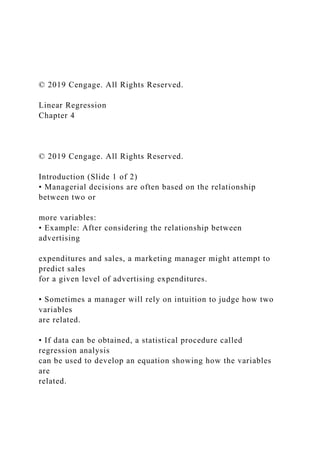
Figure 2.1 - Dow Jones Index Values Since 2002
8
Vb
Bm
Mbm
Example: (contd.)
Time series data: Figure 2.1 illustrates that the DJI was near
10,000 in 2002 and climbed to above 14,000 in 2007. However,
the financial crisis in 2008 led to a significant decline in the
DJI to between 6000 and 7000 by 2009. Since 2009, the DJI has
been generally increasing and topped 14,000 in April 2013.
8
Types of Data
9
Sources of data

Experimental study - A variable of interest is first identified.
Then one or more other variables are identified and controlled
or manipulated so that data can be obtained about how they
influence the variable of interest.
Nonexperimental study or observational study - Make no
attempt to control the variables of interest.
A survey is perhaps the most common type of observational
study.
Vb
Bm
Mbm
Example:
Experimental study:
If a pharmaceutical firm is interested in conducting an
experiment to learn about how a new drug affects blood
pressure, then blood pressure is the variable of interest in the
study.
The dosage level of the new drug is another variable that is
hoped to have a causal effect on blood pressure.
To obtain data about the effect of the new drug, researchers
select a sample of individuals.
The dosage level of the new drug is controlled as different
groups of individuals are given different dosage levels.
Before and after the study, data on blood pressure are collected
for each group.
Statistical analysis of these experimental data can help

determine how the new drug affects blood pressure.
9
Figure 2.2 - Customer Opinion Questionnaire used by Chops
City Grill Restaurant
10
Vb
Bm
Mbm
Example: (contd.)
Nonexperimental study:
Figure 2.2 shows a customer opinion questionnaire used by
Chops City Grill in Naples, Florida.
Note that the customers who fill out the questionnaire are asked
to provide ratings for 12 variables, including overall
experience, the greeting by hostess, the table visit by the
manager, overall service, and so on.
The response categories of excellent, good, average, fair, and
poor provide categorical data that enable Chops City Grill
management to maintain high standards for the restaurant’s food
and service.
In some cases, the data needed for a particular application
already exist from an experimental or observational study
already conducted.
Companies maintain a variety of databases about their
employees, customers, and business operations.
10

Modifying Data in Excel
11
Vb
Bm
Mbm
Table 2.2 - Top 20 Selling Automobiles in United States in
March 2011
12
Vb
Bm
Mbm
12
Figure 2.3 - Top 20 Selling Automobiles Data entered into
Excel with Percent Change in Sales from 2010
13
Vb
Bm
Mbm
Figure 2.3 shows the data from Table 2.2 entered into an Excel
spreadsheet, and the percent change in sales for each model
from March 2010 to March 2011 has been calculated.
This is done by entering the formula = (D2-E2)/E2 in cell F2

and then copying the contents of this cell to cells F3 to F20.
13
Sorting and filtering data in excel
Illustration - To sort the automobiles by March 2010 sales
Step 1: Select cells A1:F21
Step 2: Click the DATA tab in the Ribbon
Step 3: Click Sort in the Sort & Filter group
Step 4: Select the check box for My data has headers
Step 5: In the first Sort by dropdown menu, select Sales (March
2010)
Step 6: In the Order dropdown menu, select Largest to Smallest
Step 7: Click OK
14
Vb
Bm
Mbm
Figure 2.4 - Using Excel’s Sort Function to Sort the Top Selling
Automobiles Data
15
Vb
Bm
Mbm
15

Figure 2.5 - Top Selling Automobiles Data Sorted by Sales in
March 2010 Sales
16
Vb
Bm
Mbm
The result of using Excel’s Sort function for the March 2010
data is shown in Figure 2.5.
Although the Honda Accord was the best-selling automobile in
March 2011, both the Toyota Camry and the Toyota
Corolla/Matrix outsold the Honda Accord in March 2010.
Note that while Sales (March 2010), which is in column E, is
sorted, the data in all other columns are adjusted accordingly.
16
Sorting and filtering data in excel
Illustration - Using Excel’s Filter function to see the sales of
models made by Toyota.
Step 1: Select cells A1:F21
Step 2: Click the DATA tab in the Ribbon
Step 3: Click Filter in the Sort & Filter group
Step 4: Click on the Filter Arrow in column B, next to
Manufacturer
Step 5: Select only the check box for Toyota. You can easily
deselect all choices by unchecking (Select All)
17
Vb
Bm

Mbm
Figure 2.6 - Top Selling Automobiles Data Filtered to Show
Only Automobiles Manufactured by Toyota
18
Vb
Bm
Mbm
The result (Figure 2.6) is a display of only the data for models
made by Toyota.
Of the 20 top-selling models in March 2011, Toyota made three
of them.
Further filter the data by choosing the down arrows in the other
columns.
All data can be made visible again by clicking on the down
arrow in column B and checking (Select All) or by clicking
Filter in the Sort & Filter Group again from the DATA tab.
18
Conditional Formatting of Data in Excel: Makes it easy to
identify data that satisfy certain conditions in a data set.
Illustration - To identify the automobile models in Table 2.2 for
which sales had decreased from March 2010 to March 2011.
Step 1: Starting with the original data shown in Figure 2.3,
select cells F1:F21
Step 2: Click on the HOME tab in the Ribbon
19

Vb
Bm
Mbm
19
Illustration (contd.)
Step 3: Click Conditional Formatting in the Styles group
Step 4: Select Highlight Cells Rules, and click Less Than from
the dropdown menu
Step 5: Enter 0% in the Format cells that are LESS THAN: box
Step 6: Click OK
20
Vb
Bm
Mbm
20
Figure 2.7 - Using Conditional Formatting in Excel to Highlight
Automobiles with Declining Sales from March 2010
21
Vb
Bm
Mbm
Here, the models with decreasing sales (Toyota Camry, Ford

Focus, Chevrolet Malibu, and Nissan Versa) are now clearly
visible.
21
Figure 2.8 - Using Conditional Formatting in Excel to Generate
Data Bars for the Top Selling Automobiles Data
22
Vb
Bm
Mbm
We can choose Data Bars from the Conditional Formatting
dropdown menu in the Styles Group of the HOME tab in the
Ribbon.
Data bars are essentially a bar chart input into the cells that
show the magnitude of the cell values.
The width of the bars in this display are comparable to the
values of the variable for which the bars have been drawn;
a value of 20 creates a bar twice as wide as that for a value of
10.
Negative values are shown to the left side of the axis; positive
values are shown to the right.
Cells with negative values are shaded in a color different from
that of cells with positive values.
22
Creating Distributions
from Data
23

Vb
Bm
Mbm
23
Creating Distributions from Data
Frequency distributions for categorical data
Frequency distribution: A summary of data that shows the
number (frequency) of observations in each of several
nonoverlapping classes, typically referred to as bins, when
dealing with distributions.
24
Vb
Bm
Mbm
Table 2.3 - Data from a Sample of 50 Soft Drink Purchases
25
Vb
Bm
Mbm
The data in Table 2.3 is taken from a sample of 50 soft drink
purchases.
Each purchase is for one of five popular soft drinks, which
define the five bins: Coca-Cola, Diet Coke, Dr. Pepper, Pepsi,

and Sprite.
25
Table 2.4 - Frequency Distribution of Soft Drink Purchases
26
The frequency distribution summarizes information about the
popularity of the five soft drinks:
Coca-Cola is the leader, Pepsi is second, Diet Coke is third, and
Sprite and Dr. Pepper are tied for fourth.
Vb
Bm
Mbm
The frequency distribution of soft drink purchases (table 2.4) is
obtained by counting the number of times each soft drink
appears in Table 2.3.
Coca-Cola appears 19 times, Diet Coke appears 8 times, Dr.
Pepper appears 5 times, Pepsi appears 13 times, and Sprite
appears 5 times.
This frequency distribution provides a summary of how the 50
soft drink purchases are distributed across the five soft drinks.
26
Figure 2.9 - Creating a Frequency Distribution for Soft Drinks
Data in Excel
27
Vb
Bm

Mbm
Figure 2.9 shows the sample of 50 soft drink purchases in an
Excel spreadsheet.
Column D contains the five different soft drink categories as the
bins.
In cell E2, enter the formula =COUNTIF($A$2:$B$26, D2),
where A2:B26 is the range for the sample data, and D2 is the
bin (Coca-Cola) to match.
The COUNTIF function in Excel counts the number of times a
certain value appears in the indicated range.
In this case, we want to count the number of times Coca-Cola
appears in the sample data. The result is a value of 19 in cell
E2, indicating that Coca-Cola appears 19 times in the sample
data.
The formula from cell E2 to cells E3 to E6 can be copied to get
frequency counts for Diet Coke, Pepsi, Dr. Pepper, and Sprite.
By using the absolute reference $A$2:$B$26 in the formula.
27
Relative frequency and percent frequency distributions
Relative frequency distribution: It is a tabular summary of data
showing the relative frequency for each bin.
Percent frequency distribution: Summarizes the percent
frequency of the data for each bin.
Used to provide estimates of the relative likelihoods of different
values of a random variable.
28
Vb

Bm
Mbm
28
Table 2.5 - Relative Frequency and Percent Frequency
Distributions of Soft Drink Purchases
29
Vb
Bm
Mbm
Table 2.4 shows that the relative frequency for Coca-Cola is
19/50 = 0.38, the relative frequency for Diet Coke is 8/50 =
0.16, and so on.
From the percent frequency distribution, it is seen that 38
percent of the purchases were Coca-Cola, 16 percent of the
purchases were Diet Coke, and so on.
Note that 38 percent + 26 percent + 16 percent = 80 percent of
the purchases were the top three soft drinks.
29
Frequency distributions for quantitative data
Three steps necessary to define the classes for a frequency
distribution with quantitative data:
1. Determine the number of nonoverlapping bins.
2. Determine the width of each bin.
3. Determine the bin limits.
30

Vb
Bm
Mbm
Number of bins:
Bins are formed by specifying the ranges used to group the data.
Generally, use between 5 and 20 bins.
Small number of data items - five or six bins.
Larger number of data items - more bins are required.
The goal is to use enough bins to show the variation in the data,
but not so many classes that some contain only a few data items.
Width of the bins:
It should be the same for each bin.
Thus the choices of the number of bins and the width of bins are
not independent decisions.
A larger number of bins means a smaller bin width and vice
versa.
Approximate bin width =
Bin limits:
Bin limits must be chosen so that each data item belongs to one
and only one class.
The lower bin limit identifies the smallest possible data value
assigned to the bin.
The upper bin limit identifies the largest possible data value
assigned to the class.
30

31
Table 2.6 - Year-End Audit Times (Days)
Table 2.7 - Frequency, Relative Frequency, and Percent
Frequency
Distributions for the Audit Time Data
Vb
Bm
Mbm
Number of bins:
The number of data items in Table 2.6 is relatively small (n =
20). Hence, we choose to develop a frequency distribution with
five bins.
Width of bins:
The largest data value is 33, and the smallest data value is 12.
Because we decided to summarize the data with five classes,
using the expression “Approximate bin width = ”, provides an
approximate bin width of (33 – 12)/5 = 4.2.
We therefore decided to round up and use a bin width of five
days in the frequency distribution.
Bin limits:
We selected 10 days as the lower bin limit and 14 days as the
upper bin limit for the first class. This bin is denoted 10–14 in
Table 2.7.
The smallest data value, 12, is included in the 10–14 bin. We
then selected 15 days as the lower bin limit and 19 days as the
upper bin limit of the next class.

We continued defining the lower and upper bin limits to obtain
a total of five classes: 10–14, 15–19, 20–24, 25–29, and 30–34.
The difference between the upper bin limits of adjacent bins is
the bin width. Using the first two upper bin limits of 14 and 19,
we see that the bin width is 19 – 14 = 5.
With the number of bins, bin width, and bin limits determined, a
frequency distribution can be obtained by counting the number
of data values belonging to each bin.
Using the frequency distribution in Table 2.7, we can observe
that:
The most frequently occurring audit times are in the bin of 15–
19 days.
Eight of the 20 audit times are in this bin.
Only one audit required 30 or more days.
31
Figure 2.10 - Using Excel to Generate a Frequency Distribution
for Audit Times Data
32
Vb
Bm
Mbm
Figure 2.10 shows the data from Table 2.6 entered into an Excel
Worksheet.
The sample of 20 audit times is contained in cells A2:D6.
The upper limits of the defined bins are in cells A10:A14.
We can use the FREQUENCY function in Excel to count the
number of observations in each bin:

Step 1. Select cells B10:B14
Step 2. Enter the formula =FREQUENCY(A2:D6, A10:A14).
The range A2:D6 defines the data set, and the range A10:A14
defines the bins
Step 3. Press CTRL+SHIFT+ENTER
Excel will then fill in the values for the number of observations
in each bin in cells B10 through B14 because these were the
cells selected in Step 1 above.
32
Histogram: A common graphical presentation of quantitative
data
Constructed by placing the variable of interest on the horizontal
axis and the selected frequency measure (absolute frequency,
relative frequency, or percent frequency) on the vertical axis.
The frequency measure of each class is shown by drawing a
rectangle whose base is determined by the class limits on the
horizontal axis and whose height is the corresponding frequency
measure.
33
Vb
Bm
Mbm
33

Figure 2.11 - Histogram for the Audit Time Data
34
Vb
Bm
Mbm
In figure 2.11, note that the class with the greatest frequency is
shown by the rectangle appearing above the class of 15–19
days.
The height of the rectangle shows that the frequency of this
class is 8.
34
Figure 2.12 - Creating a Histogram for the Audit Time Data
using Data Analysis Toolpak in Excel
35
Vb
Bm
Mbm
Histograms can be created in Excel using the Data Analysis
ToolPak. Following are the steps to create histogram in Excel.
Step 1. Click the DATA tab in the Ribbon
Step 2. Click Data Analysis in the Analysis group
Step 3. When the Data Analysis dialog box opens, choose
Histogram from the list of Analysis Tools, and click OK
In the Input Range: box, enter A2:D6
In the Bin Range: box, enter A10:A14
Under Output Options:, select New Worksheet Ply:
Select the check box for Chart Output

Click OK
35
Figure 2.13 - Completed Histogram for the Audit Time Data
using Data Analysis ToolPak in Excel
36
Vb
Bm
Mbm
In figure 2.13, we have modified the bin ranges in column A by
typing the values shown in Figure 2.13 into cells A2:A6 so that
the chart created by Excel shows both the lower and upper
limits for each bin.
We have also removed the gaps between the columns in the
histogram in Excel to match the traditional format of
histograms.
To remove the gaps between the columns in the Histogram
created by Excel, follow these steps:
Step 1. Right-click on one of the columns in the histogram
Select Format Data Series…
Step 2. When the Format Data Series pane opens, click the
Series Options button.
Set the Gap Width to 0%
36
Histogram provides information about the shape, or form, of a
distribution.

Skewness: Lack of symmetry
Important characteristic of the shape of a distribution
37
Vb
Bm
Mbm
37
Figure 2.14 - Histograms Showing Distributions with Different
Levels of Skewness
38
Vb
Bm
Mbm
Panel A: Moderately skewed to the left
Here, tail extends farther to the left than to the right.
Example: Exam scores, with no scores above 100 percent, most
of the scores above 70 percent, and only a few really low
scores.
Panel B: Moderately skewed to the right
Tail extends farther to the right than to the left.
Example: Housing prices; a few expensive houses create the
skewness in the right tail.

Panel C: Symmetric
The left tail mirrors the shape of the right tail.
Example: Data for SAT scores, the heights and weights of
people, and so on lead to histograms that are roughly
symmetric.
Panel D: Highly skewed to the right
Example: Data on housing prices, salaries, purchase amounts,
and so on often result in histograms skewed to the right.
38
Cumulative Distributions
Cumulative frequency distribution: A variation of the frequency
distribution that provides another tabular summary of
quantitative data.
Uses the number of classes, class widths, and class limits
developed for the frequency distribution.
Shows the number of data items with values less than or equal
to the upper class limit of each class.
39
Vb
Bm
Mbm
39

Table 2.8 - Cumulative Frequency, Cumulative Relative
Frequency, and Cumulative Percent Frequency Distributions for
the Audit Time Data
40
Vb
Bm
Mbm
Consider the class with the description “Less than or equal to
24.”
The cumulative frequency for this class is simply the sum of the
frequencies for all classes with data values less than or equal to
24.
The sum of the frequencies for classes 10–14, 15–19, and 20–24
indicates that 4 + 8 + 5 = 17 data values are less than or equal
to 24. Hence, the
cumulative frequency for this class is 17.
In addition, the cumulative frequency distribution in Table 2.8
shows that four audits were completed in 14 days or less and
that 19 audits were completed in 29 days or less.
The cumulative relative frequency distribution can be computed
either by summing the relative frequencies in the relative
frequency distribution or by dividing the cumulative frequencies
by the total number of items.
Using the latter approach, we found the cumulative relative
frequencies in column 3 of Table 2.8 by dividing the cumulative
frequencies in column 2 by the total number of items (n = 20).
The cumulative percent frequencies were again computed by
multiplying the relative frequencies by 100.
The cumulative relative and percent frequency distributions
show that 0.85 of the audits, or 85 percent, were completed in
24 days or less, 0.95 of the audits, or 95 percent, were
completed in 29 days or less, and so on.

40
Measures of Location
41
Vb
Bm
Mbm
41
Mean/Arithmetic mean
Average value for a variable.
The mean is denoted by .
n = sample size
= value of variable x for the first observation
= value of variable x for the second observation
= value of variable x for the nth observation

42
Sample mean, = =
Vb
Bm
Mbm
Arithmetic Mean:
Provides a measure of central location for the data.
Denoted by for sample data.
Denoted by µ for population data.
42
Table 2.9 - Data on Home Sales in Cincinnati, Ohio, Suburb
Illustration: Computation of the mean home selling price for the
sample of 12 home sales:
43
Vb
Bm
Mbm
43
Computation of Sample Mean
Illustration: Computation of the mean home selling price for the
sample of 12 home sales:
= =
=

=
= 219,937.50
44
Vb
Bm
Mbm
44
Median: Value in the middle when the data are arranged in
ascending order.
Middle value, for an odd number of observations
Average of two middle values, for an even number of
observations
45
Vb
Bm
Mbm
45
Computation of Sample Median
Illustration - When the number of observations are odd
Consider the class size data for a sample of five college classes:
46 54 42 46 32
Arrange the class size data in ascending order .
32 42 46 46 54

Middlemost value in the data set = 46.
Median is 46.
46
Vb
Bm
Mbm
Because n = 5 is odd, median is the middlemost value in the
data set, 46.
46
Illustration - When the number of observations are even
Consider the data on home sales in Cincinnati, Ohio, Suburb:
47
Vb
Bm
Mbm

47
Illustration (contd.) - When the number of observations are even
Arrange the data in ascending order:
108,000 138,000 138,000 142,000 186,000 199,500 208,000
254,000 254,000 257,500 298,000 456,250
Median = average of two middle values = = 203,750
48
Middle Two Values
Vb
Bm
Mbm
Because n = 12 is even, the median is the average of the middle
two values: 199,500 and 208,000.
48
Mode: Value that occurs most frequently in a data set.
Consider the class size data:
32 42 46 46 54
Observe - 46 is the only value that occurs more than once.
Mode is 46.

Multimodal data - Data contain at least two modes.
Bimodal data - Data contain exactly two modes.
49
Vb
Bm
Mbm
49
Figure 2.15 - Calculating the Mean, Median, and Modes for the
Home Sales Data using Excel
50
Vb
Bm
Mbm
The mean can be found in Excel using the AVERAGE function.
The value for the mean in cell E2 is calculated using the
formula =AVERAGE(B2:B13).
The median of a data set can be found in Excel using the
function MEDIAN. The value for the median in cell E3 is found
using the formula =MEDIAN(B2:B13).
The Excel MODE.SNGL function will return only a single most-
often-occurring value.
For multimodal distributions, we must use the MODE.MULT
command in Excel to return more than one mode.
To find both of the modes in Excel, we take these steps:

Step 1. Select cells E4 and E5
Step 2. Enter the formula =MODE.MULT(B2:B13)
Step 3. Press CTRL+SHIFT+ENTER
Excel enters the values for both modes of this data set in cells
E4 and E5: $138,000 and $254,000.
50
Geometric mean: nth root of the product of n values
Used in analyzing growth rates in financial data.
Sample geometric mean:
= [
51
Vb
Bm
Mbm
51
Table 2.10 - Percentage Annual Returns and Growth Factors for
the Mutual Fund Data
Illustration - Consider the percentage annual returns and growth
factors for the mutual fund data over the past 10 years.
We will determine the mean rate of growth for the fund over the
10-year period.
52

Vb
Bm
Mbm
Computation of Geometric Mean
Solution
:
Product of the growth factors:
(.779)1.287)(1.109)(1.049)(1.158)(1.055)(.630)(1.265)(1.151)(1
.021)
= 1.335
Geometric mean of the growth factors:
= = 1.029
Conclude that annual returns grew at an average annual rate of
(1.029 – 1)100% or 2.9%.
53
Vb
Bm
Mbm

53
Figure 2.16 - Calculating the Geometric Mean for the Mutual
Fund Data Using Excel
54
Vb
Bm
Mbm
In Figure 2.16, the value for the geometric mean in cell C13 is
found using the formula =GEOMEAN(C2:C11).
54
Measures of Variability
55
Vb

Bm
Mbm
Range: Found by subtracting the smallest value from the largest
value in a data set.
Illustration: Consider the data on home sales in Cincinnati,
Ohio, Suburb:
56
Vb
Bm
Mbm
56
Computation of Range
Illustration (contd.):

Largest home sales price - $456,250
Smallest home sales price - $108,000
Range = Largest value – Smallest value
= $456,250 – $108,000
= $348,250
Drawback: Range is based on only two of the observations and
thus is highly influenced by extreme values.
57
Vb
Bm
Mbm

57
Variance: Measure of variability that utilizes all the data.
It is based on the deviation about the mean, which is the
difference between the value of each observation (xi) and the
mean.
The deviations about the mean are squared while computing the
variance.
Sample variance, =
Population variance , =
58
Vb
Bm
Mbm
58
Table 2.12 - Computation of Deviations and Squared Deviations
about the Mean for the Class Size Data

59
= = =
Computation of Sample Variance:
Vb
Bm
Mbm
59
Standard deviation: Positive square root of the variance
Measured in the same units as the original data.
For sample , s =
For population, σ =
Coefficient of variation:
Measures the standard deviation relative to the mean.
Expressed as a percentage.
60

Vb
Bm
Mbm
60
Computation of Coefficient of Variation
Illustration:
Consider the class size data:
46 54 42 46 32
Mean, = 44
Standard deviation, s = 8
Coefficient of variation = % = 18.2%
61
Vb
Bm
Mbm

The coefficient of variation tells that the sample standard
deviation is 18.2 percent of the value of the sample mean.
61
Figure 2.18 - Calculating Variability Measures for the Home
Sales Data in Excel
62
Vb
Bm
Mbm
Calculating the variability measures in Excel:
Range:
The range can be calculated in Excel using the MAX and MIN
functions.
The range value in cell E7 of Figure 2.18 calculates the range
using the formula =MAX(B2:B13) - MIN(B2:B13).
This subtracts the smallest value in the range B2:B13 from the
largest value in the range B2:B13.
Variance:

The variance in cell E8 is calculated using the formula
=VAR.S(B2:B13).
Excel calculates the variance of the sample of 12 home sales to
be 9,037,501,420.
Standard deviation:
The sample standard deviation in cell E9 is calculated using the
formula =STDEV.S(B2:B13).
Excel calculated the sample standard deviation for the home
sales to be $95,065.77.
Coefficient of Variation:
It is calculated in cell E11 using the formula =E9/E2, which
divides the standard deviation by the mean. The coefficient of
variation for the home sales data is 43.22 percent.
62
Analyzing
Distributions

63
Vb
Bm
Mbm
Analyzing Distributions
Percentile: Value of a variable at which a specified
(approximate) percentage of observations are below that value.
The pth percentile tells us the point in the data where:
Approximately p percent of the observations have values less
than the pth percentile;
Approximately (100 – p) percent of the observations have
values greater than the pth percentile.
64
Vb
Bm
Mbm
64

Analyzing Distributions
Steps to calculate the pth percentile:
Arrange the data in ascending order (smallest to largest value).
Compute k = (n + 1) × p.
Divide k into its integer component, i, and its decimal
component, d.
If d = 0, find the kth largest value in the data set. This is the pth
percentile.
(contd.)
65
Vb
Bm
Mbm
65
Analyzing …

Chapter 3
Data Visualization
1
Vb
Bm
Mbm
Introduction
Data visualization involves:
Creating a summary table for the data.
Generating charts to help interpret, analyze, and learn from the
data.
Uses of data visualization:
Helpful for identifying data errors.
Reduces the size of your data set by highlighting important
relationships and trends in the data.

2
Vb
Bm
Mbm
2
Overview of Data
Visualization
3
Vb
Bm
Mbm
Overview of Data Visualization
Data-ink ratio: Measures the proportion of what Tufte terms
“data-ink” to the total amount of ink used in a table or chart.
Edward R. Tufte first described the data-ink ratio.
Helpful for creating effective tables and charts for data

visualization.
Data-ink - Ink used in a table or chart that is necessary to
convey the meaning of the data to the audience.
Non-data-ink - Ink used in a table or chart that serves no useful
purpose in conveying the data to the audience.
4
Vb
Bm
Mbm
Table 3.1 - Example of a Low Data-Ink Ratio Table
and
Figure 3.3 - Example of a Low Data-Ink Ratio Chart
5

Vb
Bm
Mbm
Let us consider the case of Gossamer Industries, a firm that
produces fine silk clothing products.
Gossamer is interested in tracking the sales of one of its most
popular items, a particular style of women’s scarf.
Table 3.1 and Figure 3.3 provide examples of a table and chart
with low data-ink ratios used to display sales of this style of
women’s scarf.
The data used in this table and figure represent product sales by
day.
5
Table 3.2 - Increasing the Data-Ink Ratio by Removing
Unnecessary Gridlines
and
Figure 3.4 - Increasing the Data-Ink Ratio by Adding Labels to
Axes and
Removing Unnecessary Lines and Labels
6

Vb
Bm
Mbm
Table 3.2 shows a modified table in which all grid lines have
been deleted except for those around the title of the table.
Deleting the grid lines in Table 3.1 increases the data-ink ratio
because a larger proportion of the ink used in the table is used
to convey the information
(the actual numbers).
Similarly, deleting the unnecessary horizontal lines in Figure
3.4 increases the data-ink ratio.
6
Tables
7

Vb
Bm
Mbm
7
Tables
Tables should be used when:
1. The reader needs to refer to specific numerical values.
2. The reader needs to make precise comparisons between
different values and not just relative comparisons.
3. The values being displayed have different units or very
different magnitudes.
8
Vb
Bm
Mbm
8

Tables
9
Table 3.3 - Table showing Exact Values for Costs and Revenues
by Month for Gossamer Industries
Figure 3.5 - Line Chart of Monthly Costs and Revenues at
Gossamer Industries
Vb
Bm
Mbm
Consider when the accounting department of Gossamer
Industries is summarizing the company’s annual data for
completion of its federal tax forms.
In this case, the specific numbers corresponding to revenues and
expenses are important and not just the relative values.
Therefore, these data should be presented in a table similar to
Table 3.3.
Similarly, if it is important to know exactly by how much
revenues exceed expenses each month, then this would also be
better presented as a table rather than as a line chart, as seen in

Figure 3.5.
9
Figure 3.6 - Combined Line Chart and Table for Monthly Costs
and Revenues at Gossamer Industries
10
Vb
Bm
Mbm
Figure 3.6 allows the reader to easily see the monthly changes
in revenues and costs while also being able to refer to the exact
numerical values.
10
Table 3.4 - Table displaying Headcount, Costs, and Revenues at

Gossamer Industries
11
Vb
Bm
Mbm
Costs and revenues are measured in dollars ($), but head count
is measured in number of employees.
Although all these values can be displayed on a line chart using
multiple vertical axes, this is generally not recommended.
Because the values have widely different magnitudes (costs and
revenues are in the tens of thousands, whereas headcount is
approximately 10 each month), it would be difficult to interpret
changes on a single chart.
Therefore, a table similar to Table 3.4 is recommended.
11
Tables
Table Design Principles:
Avoid using vertical lines in a table unless they are necessary
for clarity.
Horizontal lines are generally necessary only for separating

column titles from data values or when indicating that a
calculation has taken place.
12
Vb
Bm
Mbm
12
Figure 3.7 - Comparing different Table Designs
13
Vb
Bm
Mbm
Figure 3.7 compares several forms of a table displaying

Gossamer’s costs and revenue data.
Most people find Design D, with the fewest grid lines, easiest to
read.
In this table, grid lines are used only to separate the column
headings from the data and to indicate that a calculation has
occurred to generate the Profits row and the Total column.
13
Table 3.5 - Larger Table Showing Revenues by Location for 12
Months of Data
14
Vb
Bm
Mbm
Table 3.5 breaks out the revenue data by location for nine cities
and shows 12 months of revenue and cost data.
Every other column has been lightly shaded. This helps the
reader quickly scan the table to see which values correspond
with each month.
The horizontal line between the revenue for Academy and the

Total row helps the reader differentiate the revenue data for
each location and indicates that a calculation has taken place to
generate the totals by month.
Columns of numerical values in a table should be right-aligned.
This makes it easy to see differences in the magnitude of
values.
If you are showing digits to the right of the decimal point, all
values should include the same number of digits to the right of
the decimal.
It is generally best to left-align text values within a column in a
table, as in the Revenues by Location (the first) column of
Table 3.5.
Column headings should either match the alignment of the data
in the columns or be centered over the values, as in Table 3.5.
14
Tables
15
Crosstabulation: A useful type of table for describing data of
two variables.
PivotTable: A crosstabulation in Microsoft Excel.

Vb
Bm
Mbm
15
Table 3.6 - Quality Rating and Meal Price for 300 Los Angeles
Restaurants
16

Vb
Bm
Mbm
Data on the quality rating, meal price, and the usual wait time
for a table during peak hours were collected for a sample of 300
Los Angeles area restaurants.
Table 3.6 shows the data for the first ten restaurants.
Quality ratings - categorical data; Meal prices - quantitative
data.
16
Table 3.7 - Crosstabulation of Quality Rating and Meal Price
for 300 Los Angeles Restaurants
17
The greatest number of restaurants in the sample (64) have a
very good rating and a meal price in the $20–29 range.
Only two restaurants have an excellent rating and a meal price
in the $10–19 range.
The right and bottom margins of the crosstabulation give the

frequency of quality rating and meal price separately.
Vb
Bm
Mbm
A crosstabulation of the data for quality rating and meal price
data is shown in Table 3.7.
The left and top margin labels define the classes for the two
variables. In the left margin, the row labels (Good, Very Good,
and Excellent) correspond to the three classes of the quality
rating variable.
In the top margin, the column labels ($10–19, $20–29, $30–39,
and $40–49) correspond to the four classes (or bins) of the meal
price variable.
Each restaurant in the sample provides a quality rating and a
meal price.
For example, restaurant 5 is identified as having a very good
quality rating and a meal price of $33. This restaurant belongs
to the cell in row 2 and column 3.
From the right margin, we see that data on quality ratings show
84 good restaurants, 150 very good restaurants, and 66 excellent
restaurants. Similarly, the bottom margin shows the counts for

the meal price variable. The value of 300 in the bottom right
corner of the table indicates that 300 restaurants were included
in this data set.
In constructing a crosstabulation, we simply count the number
of restaurants that belong to each of the cells in the
crosstabulation.
17
Figure 3.8 - Excel Worksheet Containing Restaurant Data
18
Vb
Bm
Mbm
Figure 3.8 illustrates Zagat’s restaurant data in Excel.
Each of the four columns in Figure 3.8 [Restaurant, Quality
Rating, Meal Price ($), and Wait Time (min)] is considered a

field by Excel.
18
Figure 3.9 - Initial PivotTable Field List and PivotTable Field
Report for the Restaurant Data
19
Vb
Bm
Mbm
To create a PivotTable in Excel, we follow these steps:
Step 1: Click the INSERT tab on the Ribbon
Step 2: Click PivotTable in the Tables group
Step 3: When the Create PivotTable dialog box appears:
Choose Select a Table or Range
Enter A1:D301 in the Table/Range: box
Select New Worksheet as the location for the PivotTable Report
Click OK
The resulting initial PivotTable Field List and PivotTable
Report are shown in Figure 3.9.

19
Figure 3.10 - Completed PivotTable Field List and A Portion of
the PivotTable Report for the Restaurant Data (Columns H:AK
are Hidden)
20
Vb
Bm
Mbm
Fields may be chosen to represent rows, columns, or values in
the body of the PivotTable Report.
The following steps show how to use Excel’s PivotTable Field
List to assign the Quality Rating field to the rows, the Meal
Price ($) field to the columns, and the Restaurant field to the
body of the PivotTable report.
Step 4: In the PivotTable Fields area, go to Drag fields between
areas below:
Drag the Quality Rating field to the ROWS area

Drag the Meal Price ($) field to the COLUMNS area
Drag the Restaurant field to the VALUES area
Step 5: Click on Sum of Restaurant in the VALUES area
Step 6: Select Value Field Settings from the list of options
Step 7: When the Value Field Settings dialog box appears:
Under Summarize value field by, select Count
Click OK
Figure 3.10 shows the completed PivotTable Field List and a
portion of the PivotTable worksheet as it now appears.
20
Figure 3.11 - Final PivotTable Report for the Restaurant Data
21
Vb
Bm
Mbm
To complete the PivotTable, we need to group the columns
representing meal prices and place the row labels for quality
rating in the proper order:

Step 8: Right-click in cell B4 or any cell containing a meal
price column label
Step 9: Select Group from the list of options
Step 10: When the Grouping dialog box appears:
Enter 10 in the Starting at: box
Enter 49 in the Ending at: box
Enter 10 in the By: box
Click OK
Step 11: Right-click on “Excellent” in cell A5
Step 12: Select Move and click Move “Excellent” to End
The final PivotTable, shown in Figure 3.11, provides the same
information as the crosstabulation in Table 3.7.
For instance, row 8 provides the frequency distribution for the
data over the quantitative variable of meal price.
Seventy-eight restaurants have meal prices of $10 to $19.
Column F provides the frequency distribution for the data over
the categorical variable of quality.
One hundred fifty restaurants have a quality rating of Very
Good.
21
Figure 3.12 - Percent Frequency Distribution as a PivotTable

for the Restaurant Data
22
Vb
Bm
Mbm
Percent frequency distribution for the restaurant data can be
created using a PivotTable by using the following steps:
Step 1: Click the Count of Restaurant in the VALUES area
Step 2: Select Value Field Settings… from the list of options
Step 3: When the Value Field Settings dialog box appears, click
the tab for Show Values As
Step 4: In the Show values as area, select % of Grand Total
from the drop-down menu
Click OK
Figure 3.12 displays the percent frequency distribution for the
Restaurant data as a Pivot-Table.
The figure indicates that 50 percent of the restaurants are in the
Very Good quality category and that 26 percent have meal
prices between $10 and $19.

22
Figure 3.13 - PivotTable Report for the Restaurant Data with
Average Wait Times Added
23
Vb
Bm
Mbm
PivotTables may be used to display statistics other than a
simple count of items.
Figure 3.11 to display summary information on wait times
instead of meal prices.
Step 1: Click the Count of Restaurant field in the VALUES area
Select Remove Field
Step 2: Drag the Wait Time (min) to the VALUES area
Step 3: Click on Sum of Wait Time (min) in the VALUES area
Step 4: Select Value Field Settings… from the list of options
Step 5: When the Value Field Settings dialog box appears:
Under Summarize value field by, select Average

Click Number Format
In the Category: area, select Number
Enter 1 for Decimal places:
Click OK
When the Value Field Settings dialog box reappears, click OK
The completed PivotTable appears in Figure 3.13.
This PivotTable replaces the counts of restaurants with values
for the average wait time for a table at a restaurant for each
grouping of meal prices ($10–19, $20–29, $30–39, $40–49).
For instance, cell B7 indicates that the average wait time for a
table at an Excellent restaurant with a meal price of $10–$19 is
25.5 minutes.
Column F displays the total average wait times for tables in
each quality rating category.
We see that Excellent restaurants have the longest average waits
of 35.2 minutes and that Good restaurants have average wait
times of only 2.5 minutes.
Finally, cell D7 shows us that the longest wait times can be
expected at Excellent restaurants with meal prices in the $30–
$39 range (34 minutes).
23
Charts

24
Vb
Bm
Mbm
24
Charts
Charts (or graphs): Visual methods of displaying data.
Scatter chart: Graphical presentation of the relationship between
two quantitative variables.
Trendline – A line that provides an approximation of the
relationship between the variables.
Line chart: A line connects the points in the chart.
Useful for time series data collected over a period of time.
(minutes, hours, days, years, etc.)
25

Vb
Bm
Mbm
25
Table 3.8 - Sample Data for the
San Francisco Electronics Store
26
Vb
Bm
Mbm
We will investigate whether a relationship exists between the
number of commercials shown and sales at the store the
following week using a scatter chart.
The steps involved to create a scatter chart using Excel’s chart
tools are as follows:

Copy the data in the file electronics to a new excel worksheet in
columns A through C and rows 1 through 11.
Step 1: Select cells B2:C11
Step 2: Click the INSERT tab in the Ribbon
Step 3: Click the Insert Scatter (X,Y) or Bubble Chart button in
the Charts group
Step 4: When the list of scatter chart subtypes appears, click the
Scatter button
Step 5: Click the DESIGN tab under the Chart Tools Ribbon
Step 6: Click Add Chart Element in the Chart Layouts group
Select Chart Title, and click Above Chart
Click on the text box above the chart, and replace the text with
Scatter Chart for the San Francisco electronics Store
Select Axis Title, and click Primary Vertical
Click on the text box under the horizontal axis, and replace
“Axis
Title” with number of Commercials
Select Axis Title, and click Primary Horizontal
Click on the text box next to the vertical axis, and replace “Axis
Title” with Sales ($100s)
Step 9: Right-click on the one of the horizontal grid lines in the
body of the chart, and click Delete

Step 10: Right-click on the one of the vertical grid lines in the
body of the chart, and click Delete
To add a linear trendline using Excel, we use the following
steps:
Step 1: Right-click on one of the data points in the scatter chart,
and select Add Trendline…
Step 2: When the Format Trendline task pane appears, select
Linear under TRENDLINE OPTIONS
26
Figure 3.14 - Scatter Chart for the San Francisco Electronics
Store
27
Vb
Bm
Mbm
The number of commercials (x) is shown on the horizontal axis,
and sales (y) are shown on the vertical axis.

For week 1, x = 2 and y = 50. A point is plotted on the scatter
chart at those coordinates; similar points are plotted for the
other nine weeks.
Note that during two of the weeks, one commercial was shown,
during two of the weeks, two commercials were shown, and so
on.
The completed scatter chart in Figure 3.14 indicates a positive
linear relationship (or positive correlation) between the number
of commercials and sales: higher sales are associated with a
higher number of commercials.
27
Table 3.9 - Monthly Sales Data of Air Compressors at Kirkland
Industries
28
Vb
Bm
Mbm
Table 3.9 contains total sales amounts (in $100s) for air
compressors during each month in the most recent calendar
year. To create the line chart to this data, the steps are as

follows:
Copy the data in the file Kirkland to a new excel worksheet in
columns A and B; rows 1 through 13.
Step 1: Select cells A2:B13
Step 3: Click the Insert Line Chart button in the Charts group
Step 4: When the list of line chart subtypes appears, click the
Line with Markers button under 2-D Line
This creates a line chart for sales with a basic layout and
minimum formatting
Step 5: Select the line chart that was just created to reveal the
CHART TOOLS Ribbon
Click the DESIGN tab under the CHART TOOLS Ribbon
Select Axis Title from the drop-down menu
Click Primary Vertical
Title” with Sales ($100s)
Select Chart Title from the drop-down menu
Click Above Chart
Click on the text box above the chart, and replace “Chart Title”
with line Chart for Monthly Sales data
Step 8: Right-click on one of the horizontal lines in the chart,
and click Delete

28
Figure 3.15 - Scatter Chart and Line Chart for Monthly Sales
Data at Kirkland Industries
29
Vb
Bm
Mbm
29
Table 3.10 - Regional Sales Data by Month for Air Compressors
at Kirkland Industries
30
Vb
Bm
Mbm

30
Figure 3.16 - Line Chart of Regional Sales Data at Kirkland
Industries
31
Vb
Bm
Mbm
We can create a line chart in Excel that shows sales in both
regions, as in Figure 3.16, by following similar steps but
selecting cells A2:C14 in the file KirklandRegional before
creating the line chart.
Sales in both the North and South regions seemed to follow the
same increasing/decreasing pattern until October.
Starting in October, sales in the North continued to decrease
while sales in the South increased.

We would probably want to investigate any changes that
occurred in the North region around October.
31
Charts
Sparkline - Special type of line chart
Minimalist type of line chart that can be placed directly into a
cell in Excel.
Contain no axes; they display only the line for the data.
Take up very little space, and they can be effectively used to
provide information on overall trends for time series data.
32
Vb
Bm
Mbm

To create a sparkline in Excel:
Step 2: Click Line in the Sparklines group
Step 3: When the Create Sparklines dialog box opens,
Enter B3:B14 in the Data Range: box
Enter B15 in the Location Range: box
Click OK
Step 4: Copy cell B15 to cell C15
32
Figure 3.17 - Sparklines for the Regional Sales Data at Kirkland
Industries
33
Vb
Bm
Mbm
The sparklines in cells B15 and C15 do not indicate the
magnitude of sales in the North and South regions, but they do

show the overall trend for these data.
Sales in the North appear to be decreasing in recent time, and
sales in the South appear to be increasing overall.
Because sparklines are input directly into the cell in Excel, we
can also type text directly into the same cell that will then be
overlaid on the sparkline, or we can add shading to the cell,
which will appear as the background.
In Figure 3.17, we have shaded cells B15 and C15 to highlight
the sparklines.
As can be seen, sparklines provide an efficient and simple way
to display basic information about a time series.
33
Charts
Bar Charts: Use horizontal bars to display the magnitude of the
quantitative variable.
Column Charts: Use vertical bars to display the magnitude of
the quantitative variable.
Bar and column charts are very helpful in making comparisons
between categorical variables.

34
Vb
Bm
Mbm
34
Figure 3.18 - Bar Charts for Accounts Managed Data
35
Gentry manages the greatest number of accounts and Williams
the fewest.
Vb
Bm
Mbm
Consider the regional supervisor who wants to examine the

number of accounts being handled by each manager. Figure 3.18
shows a bar chart created in Excel displaying these data. To
create this bar chart in Excel:
Step 3: Click the Insert Bar Chart button in the Charts group
Step 4: When the list of bar chart subtypes appears:
Click the Clustered Bar button in the 2-D Bar section
Step 5: Select the bar chart that was just created to reveal the
CHART TOOLS ribbon
Click Primary Horizontal
Title” with Accounts Managed
Title” with Manager
Select Chart Title from the drop-down menu
Click Above Chart

with Bar Chart of Accounts Managed
Step 9: Right-click on one of the vertical lines in the chart, and
click Delete
35
Figure 3.19 - Sorted Bar Chart for Accounts Managed Data
36
Vb
Bm
Mbm
We can make the bar chart in Figure 3.18 even easier to read by
ordering the results by the number of accounts managed.
In the completed bar chart in Excel, shown in Figure 3.19, we
can easily compare the relative number of accounts managed for
all managers.
We can do this with the following steps:
Step 2: Right-click any of the cells A1:B9
Choose Sort
Click Custom Sort

Step 3: When the Sort dialog box appears:
Make sure that the check box for My data has headers is
checked
Choose Accounts Managed in the Sort by box under Column
Choose Smallest to Largest under Order
Click OK
36
Figure 3.20 - Bar Chart with Data Labels for Accounts Managed
Data
37
Vb
Bm
Mbm
In order to interpret from the bar chart exactly how many
accounts are assigned to each manager, we add data labels to
the bar chart, as in Figure 3.20, which is created in Excel using
the following steps:
Step 1: Select the bar chart just created to reveal the CHART

TOOLS Ribbon
Step 2: Click DESIGN tab in the CHART TOOLS Ribbon
Select Data Labels
Click Outside End
This adds labels of the number of accounts managed to the end
of each bar so that the reader can easily look up exact values
displayed in the bar chart.
37
Charts
Pie charts: Common form of chart used to compare categorical
data.
Bubble chart: Graphical means of visualizing three variables in
a two-dimensional graph.
Sometimes a preferred alternative to a 3-D graph.
Heat map: A two-dimensional graphical representation of data
that uses different shades of color to indicate magnitude.

38
Vb
Bm
Mbm
38
Figure 3.21 - Pie Chart of Accounts Managed
39
Vb
Bm
Mbm
Figure 3.21 displays the data for the number of accounts
managed in Figure 3.18.
Visually, it is still relatively easy to see that Gentry has the
greatest number of accounts and that Williams has the fewest.
However, it is difficult to say whether Lopez or Francois has

more accounts. Research has shown that people find it very
difficult to perceive differences in area.
Compare Figure 3.21 to Figure 3.19.
Making visual comparisons is much easier in the bar chart than
in the pie chart (particularly when using a limited number of
colors for differentiation).
39
Table 3.11 - Sample Data on Billionaires
per Country
40
Vb
Bm
Mbm
Suppose that we want to compare the number of billionaires in
various countries.
Table 3.11 provides a sample of six countries, showing, for each
country, the number of billionaires per 10 million residents, the
per capita income, and the total number of billionaires.

40
Figure 3.22 - Bubble Chart Comparing Billionaires by Country
41
Vb
Bm
Mbm
Figure 3.22 shows the bubble chart that has been created by
Excel.
Copy the sample data on billionaires from the webfile
Billionaires to an Excel worksheet from columns A through D
and rows 1 through 7.
Step 1: Select cells B2:D7
Step 3: In the Charts group, click Insert Scatter (X,Y) or Bubble
Chart button
In the Bubble subgroup, click the Bubble button
Step 4: Select the chart that was just created to reveal the
CHART TOOLS ribbon

Choose Axis Title from the drop-down menu
Click Primary Horizontal
Click on the text box under the horizontal axis, and replace
“Axis Title” with Billionaires per 10 Million residents
Choose Axis Title from the drop-down menu
Title” with Per Capita income
Choose Chart Title from the drop-down menu
Click Above Chart
with Billionaires by Country
Choose Gridlines from the drop-down menu
Deselect Primary Major Horizontal and Primary Major Vertical
to remove the gridlines from the bubble chart
However, we can make this chart much more informative by
taking a few additional steps to add the names of the countries:
Choose Data Labels from the drop-down menu

Click More Data Label Options . . .
Step 10: Click the Label Options icon
Under LABEL OPTIONS, select Value from Cells, and click the
Select Range button
Step 11: When the Data Label Range dialog box opens, select
cells A2:A7 in the Worksheet.
This will enter the value “=SheetName!$A$2:$A$7” into the
Select Data Label Range box
where “SheetName” is the name of the active Worksheet
Click OK
Step 12: In the Format Data Labels task pane, deselect Y Value
in the LABEL OPTIONS area, and select Right under Label
Position
41
Figure 3.23 - Bubble Chart Comparing Billionaires by Country
with Data Labels added
42
Vb

Bm
Mbm
The completed bubble chart in Figure 3.23 enables us to easily
associate each country with the corresponding bubble.
Hong Kong has the most billionaires per 10 million residents
but that the United States has many more billionaires overall
(Hong Kong has a much smaller population than the United
States).
From the relative bubble sizes, we see that China and Russia
also have many billionaires but that there are relatively few
billionaires per 10 million residents in these countries and that
these countries overall have low per capita incomes.
The United Kingdom, United States, and Hong Kong all have
much higher per capita incomes.
42
Figure 3.24 - Heat Map and Sparklines for Same-Store Sales
Data
43
Vb
Bm

Mbm
Figure 3.24 can be created in Excel by following these steps:
Step 1: Select cells B2:M17
Step 2: Click the HOME tab on the Ribbon
Step 3: Click Conditional Formatting in the Styles group
Choose Color Scales and click on Blue–White–Red Color Scale
To add the sparklines in Column N, we use the following steps:
Step 4: Select cell N2
Step 6: Click Line in the Sparklines group
Step 7: When the Create Sparklines dialog box opens:
Enter B2:M2 in the Data Range: box
Enter N2 in the Location Range: box and click OK
Step 8: Copy cell N2 to N3:N17
The heat map in Figure 3.24 helps the reader to easily identify
trends and patterns.
The cells shaded grey in Figure 3.24 indicate declining same-
store sales for the month, and cells shaded blue indicate
increasing same-store sales for the month. Column N in Figure
3.24 also contains sparklines for the same-store sales data.
We can see that Austin has had positive increases throughout

the year, while Pittsburgh has had consistently negative same-
store sales results.
Same-store sales at Cincinnati started the year negative but then
became increasingly positive after May.
In addition, we can differentiate between strong positive
increases in Austin and less substantial positive increases in
Chicago by means of color shadings.
A sales manager could use the heat map in Figure 3.24 to
identify stores that may require intervention and stores that may
be used as Models.
To avoid problems with interpreting differences in color, we
can add the sparklines in Column N of Figure 3.24.
43
Charts
Additional charts for multiple variables
Stacked column chart: Allows the reader to compare the relative
values of quantitative variables for the same category in a bar
chart.
Clustered column (or bar) chart: An alternative chart to stacked

column chart for …
Spreadsheet Models
Chapter 7
Introduction
• Spreadsheet models are mathematical and logic-based models.
• Referred to as what-if models:
• Provide easy-to-use, sophisticated mathematical and logical
functions.
• Allow for easy instantaneous recalculation for a change in
model inputs.
• Are less expensive.

• Often come preloaded on computers.
• Are fairly easy to use.
• The most used business analytics tool.
Building Good Spreadsheet
Models
Influence Diagrams
Building a Mathematical Model
Spreadsheet Design and Implementing the Model in a
Spreadsheet
Building Good Spreadsheet Models (Slide 1 of 11)
• Total cost of manufacturing a product is the sum of two costs:

• Fixed cost: Portion of the total cost that does not depend on
the
production quantity and remains the same no matter how much
is
produced.
• Variable cost: Portion of the total cost that is dependent on
and varies
with the production quantity.
• Make-versus-buy decision: comparing the costs of
manufacturing
in-house to the costs of outsourcing production to another firm.
Influence Diagrams:
• An influence diagram is a visual representation that shows
which entities
influence others in a model.

• Parts of the model are represented by circular or oval symbols
called
nodes, and arrows connecting the nodes show influence.
Figure 10.1: An Influence Diagram
for Nowlin’s Manufacturing Cost
Figure 10.2: An Influence
Diagram for Comparing
Manufacturing Versus
Outsourcing Cost for
Nowlin Plastics

Building a Mathematical Model:
• Consider the cost of manufacturing the required units of the
Viper.
• As the influence diagram shows, this cost is a function of the
fixed cost,
the variable cost per unit, and the quantity required.
• Define notation for every node in the influence diagram:
q = quantity (number of units) required.
FC = the fixed cost of manufacturing.
VC = the per-unit variable cost of manufacturing.
( )TMC q = total cost to manufacture q units.

Building a Mathematical Model (cont.):
• The cost-volume model for producing q units is:
• For the Viper, FC = $234,000 and VC = $2, so:
( ) $234,000 $2TMC q q= +
• Mathematical model for purchasing q units is:
• P = the per unit purchase cost:
= the total cost to outsource or purchase q units
• For the Viper, since
( )TPC q
( )$3.50, $3.5 .P TCP q q= =

Building a Mathematical Model (cont.):
• Mathematical model for the savings associated with
outsourcing:
the savings due to outsourcing
• Nowlin has to decide: For what quantities is it more cost-
effective to
outsource rather than produce the Viper?
• Mathematically, this question is: For what values of q is
( )S q =

Spreadsheet:
• For the Nowlin Plastics problem, we have defined the
following
components: q, FC, VC, ( ) ( ) ( ), , , .TMC q P TPC q S q
• TMC, TPC, and S are the functions of other components,
whereas q, FC,
VC, and P are not.
• TMC, TPC, and S will be formulas involving other cells in the
spreadsheet
model, whereas q, FC, VC, and P will just be entries in the
spreadsheet.
Spreadsheet
(cont.):
• The number of Vipers to make or buy for next year is really a

decision
Nowlin gets to make, hence we refer to quantity q as a decision
variable.
• FC, VC, and P are measurable factors that define
characteristics of the
process we are modelling; hence, we refer to FC, VC, and P as
parameters.
Figure 10.3: Nowlin Plastics
Make-Versus-Buy
Spreadsheet Model

Spreadsheet
(cont.):
• The general principles of spreadsheet model design and
construction are:
• Separate the parameters from the model: This enables the user
to update
the model parameters without the risk of mistakenly creating an
error in a
formula.
• Document the model and use proper formatting and color as
needed: A
good spreadsheet model is well documented. Clear labels and
proper
formatting and alignment facilitate navigation and
understanding.
• Use simple formulas: Clear, simple formulas can reduce errors
and make
maintaining the spreadsheet easier. Long and complex
calculations should
be divided into several cells.

What-If Analysis
Data Tables
Goal Seek
Scenario Manager
What-If Analysis (Slide 1 of 14)
Data Tables:
• Data Table: Excel tool which quantifies the impact of
changing the value
of a specific input on an output of interest.
• One-way data table: Summarizes a single input’s impact on
the output.
• Two-way data table: Summarizes two inputs’ impact on the

output.
Figure 10.4: The Input for
Constructing a One-Way
Data Table for Nowlin
Plastics
Figure 10.5 Results of One-
Way Data Table for Nowlin
Plastics

Figure 10.6: The
Input for
Constructing a
Two-Way Data
Table for Nowlin
Plastics
Figure 10.7: Results of Two-Way Data Table for Nowlin
Plastics

Goal Seek:
• Goal Seek: Excel tool that allows the user to determine the
value of an
input cell that will cause the value of a related output cell to
equal some
specified value (the goal).
• In the case of Nowlin Plastics, suppose we want to know the
value of the
quantity of Vipers where it becomes more cost effective to
manufacture
rather than outsource.
Figure 10.8: Goal Seek
Dialog Box for Nowlin
Plastics

Figure 10.9: Results from
Goal Seek for Nowlin
Plastics
Scenario Manager:
• Scenario Manager: Excel tool that quantifies the impact of
changing
multiple inputs (a setting of these multiple inputs is called a
scenario) on
one or more outputs of interest.
• Scenario Manager extends the data table concept to cases
when you are
interested in changing more than two inputs and want to

quantify the
changes these inputs have on one or more outputs of interest.
Figure 10.10:
Middletown Amusement
Park Daily Profit Model
Table 10.1: Weather Scenarios for Middletown Amusement Park
Scenarios
Partly Cloudy Rain Sunny
Season-pass Holders 3000 1200 8000

Admissions 1600 250 2400
Average Expenditure –
Season-Pass Holders $15 $10 $18
Average Expenditure –
Admissions $45 $20 $57
Cost of Operations $33,000 $27,000 $37,000
Figure 10.11:
Scenario Manager Dialog Box
Figure 10.12:
Add Scenario Dialog Box

Figure 10.13:
Scenario Values Dialog Box
Figure 10.14:
Scenario Summary Dialog Box
Figure 10.15: Scenario Summary for Middletown Amusement
Park
Some Useful Excel Functions for
Modeling

SUM and SUMPRODUCT
IF and COUNTIF
VLOOKUP
Some Useful Excel Functions for Modeling
(Slide 1 of 6)
SUM and SUMPRODUCT:
• SUM: Function that adds up all of the numbers in a range of
cells.
• SUMPRODUCT: Function that returns the sum of the products
of
elements in a set of arrays.

Figure 10.16: What-If Model
for Foster Generators
(Slide 2 of 6)
(Slide 3 of 6)
IF and COUNTIF:
• =IF(condition, result if condition is true, result if condition is
false).
• =COUNTIF(range, condition).
• Counts the number of components having a positive order
quantity.
Illustration:
• Gambrell Manufacturing produces car stereos.
• Gambrell likes to keep its components inventory to a

minimum.
• Hence, it uses an inventory policy known as an order-up-to
policy.
• Order-up-to policy: Whenever the inventory on hand drops
below a certain
level, enough units are ordered to return the inventory to that
predetermined level.
Figure 10.17: Gambrell
Manufacturing Component
Ordering Model
(Slide 4 of 6)

(Slide 5 of 6)
VLOOKUP
• This function allows the user to pull a subset of data from a
larger table
of data based on some criterion.
• General form =VLOOKUP(value, table, index, range).
where,
value = the value to search for in the first column of the table.
table = the cell range containing the table.
index = the column in the table containing the value to be
returned.
range = TRUE if looking for the first approximate match of
value and
FALSE if looking for an exact match of value.
Figure 10.18: Granite
Insurance Bonus Model

(Slide 6 of 6)
Auditing Spreadsheet Models
Trace Precedents and Dependents
Show Formulas
Evaluate Formulas
Error Checking
Watch Window
Auditing Spreadsheet Models (Slide 1 of 13)
• Excel contains a variety of tools to assist you in the

development
and debugging of spreadsheet models.
• These tools are found in the Formula Auditing group of the
Formulas tab.
Figure 10.19: The Formula Auditing Group
Trace Precedents and Dependents:
• Trace Precedents button: After selecting cells, this button
creates arrows
pointing to the selected cell from cells that are part of the

formula in that
cell.
• Trace Dependents button: Shows arrows pointing from the
selected cell
to cells that depend on the selected cell.
• Both of the tools are excellent for quickly ascertaining how
parts of a
model are linked.
Figure 10.20: Trace
Precedents for Foster
Generator

Figure 10.21: Trace
Dependents for the Foster
Generators Model
Show Formulas:
• To see the formulas in a worksheet, simply click on any cell in
the
worksheet and then click on Show Formulas—you will see the
formulas
residing in that worksheet.
• To revert to hiding the formulas, click again on the Show
Formulas
button.

Evaluate Formulas:
• The Evaluate Formulas button allows you to investigate the
calculations
of a cell in great detail.
• Provides an excellent means of identifying the exact location
of an error
in a formula.
Figure 10.22: The
Evaluate Formula Dialog
Box for Gambrell
Manufacturing

© 2019 Cengage. All Rights Reserved. Linear RegressionC.docx

Recommended

Recommended

More Related Content

Similar to © 2019 Cengage. All Rights Reserved. Linear RegressionC.docx

Similar to © 2019 Cengage. All Rights Reserved. Linear RegressionC.docx (20)

More from budbarber38650

More from budbarber38650 (20)

Recently uploaded

Recently uploaded (20)

© 2019 Cengage. All Rights Reserved. Linear RegressionC.docx