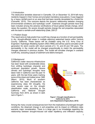
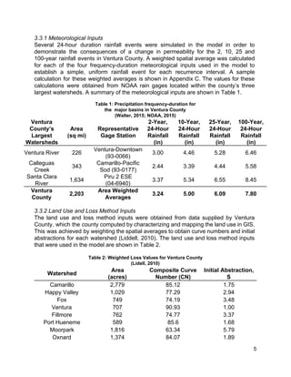
This document summarizes a study that models changes in surface runoff from drought-induced soil hydrophobicity in watersheds in Ventura County, California. The study uses the Hydrologic Modeling System (HEC-HMS) to model 11 watersheds under current conditions and potential future drought conditions. Drought is assumed to increase soil impermeability by 25%, based on previous studies. The model simulates runoff for 2, 10, 25 and 100-year storm events to compare changes in overland runoff under normal and drought conditions. Preliminary results suggest drought could significantly increase surface runoff and flooding risks by reducing soil infiltration capacity.

1.
Changes in surface runoff from drought­induced soil
hydrophobicity in the Ventura County watershed
CVEN 4323
Dr. Joseph Kasprzyk
Ariel Retuta
Cassidy Kuhn
Jack Greene

2. 1.0 Introduction
The destructive landslide observed in Camarillo, CA on December 12, 2014 left many
residents trapped in their homes and prompted mandatory evacuations. It was triggered
by a heavy rainfall event on an area that had been recently devastated by a forest fire
(Camarillo, 2015). This outcome depicts the dynamic relationship between changing
environmental conditions and hydrologic runoff . Extensive drought periods have long
been included among the adverse ramifications of future global climate change, which
raises the question: Do severe drought periods change the soil properties associated
with the basin’s rainfall­runoff relationship (Dale, 2001)?
1.1 Problem Scope
This report aims to help predict how runoff may change as a function of soil permeability
in dry, drought­affected areas in multiple adjoining watershed basins within Ventura
County, California. These basins will be modeled using the U.S. Army Corp of
Engineers’ Hydrologic Modeling System (HEC­HMS) and will be used to simulate runoff
generation for storm events with return periods of 2, 10, and 25 and 100 years. The
permeability in the model will be changed proportionally to match the permeability
changes observed in previous studies. The model will simulate changes in overland
runoff only, excluding outputs of sediment and debris transport.
2.0 Background
California’s water resource infrastructure
has been faced with considerable stress
from shifting hydrologic character and
continued population growth. Severe
climatic and hydrologic droughts have
taken hold in California over the past 10
years, with the last three years marking
some of the driest and hottest since 1985
(Mann, 2015). Much of southern
california has been characterized as
experiencing class D4 droughts, the
most severe case on the drought
classification scale, according to the
California and National Drought
Summary from 2015, as shown in dark
red in Figure 1.
Figure 1: Drought classification in
California for 2015.
(U.S. Department of Agriculture, 2015)
Among the many crucial consequences born from the implications of prolonged drought
conditions, the observed change in soil properties and its impact on infiltration rates
warrants major consideration. There is a large gap in our knowledge regarding the
relationship between drought­induced soil water repellency and infiltration capacity;
1

3. however, studies have seen significant declines in soil permeability in manually­dried
soil. The few studies that have been performed indicate that periods of severe dryness
result in hydrophobic soil conditions, which retard the runoff’s ability to infiltrate into soil
(Shakesby, 2000). As hydrophobicity is heightened in drier soil, the soil’s capacity to
infiltrate water is diminished (Shakesby, 2000). This relationship between ​hydraulic
conductivity and soil wettability is depicted in Figure 2.
Reports of reduced infiltration capacities in dry,
water­repellent soils after prescribed burning
were found to be as low as 25 times less than
in moist soils (DeBano, 1991). Other studies
observed a diminished capacity of dry sand to
infiltrate water to 1% of its capacity when
hydrophilic and moist (Wallis et. al. 1990). This
increases immediate overland runoff volumes
and may increase flooding and landslide
hazards.
The purpose of this study is to superimpose this
relationship between soil dryness and
permeability to drought­stricken soils in
California in order to identify trends of change in
overland runoff discharge. Infiltration rates and
soil permeability depends on many different
factors. Among them are soil composition, the
structure of the media, the chemical condition of
​Figure 2: Hydraulic conductivity curves ​the soil, plants/animals in the soil, and land use
for dry, hydrophobic soils (solid line) and ​(Johnson, 1963). This model will look only at one
wettable soils (dashed line). ​of these factors ­ land use. Although the model
(Shakesby, 2000) ​will output runoff values only, there is a general
consensus in the literature that reveals relationships between soil dryness and erosion.
3.0 Model
Using HEC­HMS, a regional model of the watersheds within Ventura County were
created. This model presented both current and future, drought­stricken conditions in
order to compare how overland runoff might change under extremely dry conditions.
3.1 Area of Study
Ventura County, shown in Figure 3, is a coastal area located in the south western part
of California. Its northern border is capped by the Santa Barbara National Forest and
lies just west of the Santa Susana Mountains and partially by the Santa Monica
Mountains. The Pacific Ocean borders Ventura County to the west and southwest
2

4.
Figure 3: Ventura County location within California
(City of Ventura, 2015)
The topography of Ventura County includes hilly and mountainous terrain with
elevations ranging from sea level up to 6,300 feet above sea level and is punctuated
with small valleys and alluvial fan deltas. There are eleven watershed subbasins within
the Ventura County borders that were included in the model.
Ventura County comprises three main watersheds: Ventura River at 226 square miles,
Calleguas Creek at 343 square miles, and Santa Clara River at 1,634 square miles.
3.2 Assumptions
The following simplifications and assumptions were made in this study:
● Uniform spatial distribution of rainfall for each basin for each respective rain
event and was kept constant for each time step. Storm depths for a 24­hour
storm event were obtained from the National Oceanic and Atmospheric
Administration (NOAA). Four different return periods were illustrated in the model
to compare runoff change severities across various storm intensities. The 2, 10,
25, 100­year storms were modeled.
● Uniform spatial losses for each basin and are constant for each time step.
● Uniform initial conditions for each basin.
● All water drains to ocean.
● Composite curve numbers are accurate for and representative of the entire
basin.
● Average flow for the driest month, July, was used as the base flow to simulate
drought conditions. This averaged baseflow was held constant.
● Maximally dry soil conditions were assumed to yield 25% less permeability, or
25% more imperviousness (Debano, 1991).
● Lag time was not changed as a function of soil permeability. This value remained
constant within the model.
3

5. ● Rainfall events are unaffected by drought conditions because meteorological
shifts due to climate change are difficult to quantify. This study includes a larger
rain event to simulate an extreme weather event and how the area’s changed
hydrology would behave in these conditions.
● Drought affects the entire area the same way and makes all soils uniformly
impervious.
● Changes in soil imperviousness is solely due to the degree of hydrophobicity
caused by the driest possible conditions (zero water in the vadose zone).
3.3 Model Description
Basins were delineated based on the largest population centers in the county with data
from Lindell (2010). The aerial shots of each basin can be found in Attachment D to the
report. Channel and routing information was adopted from the Ventura County
Community for a Clean Watershed website. Port Hueneme is not connected to the
watersheds of the northern part of the county ­ Port Hueneme drains directly to the
Pacific Ocean. All of the other watersheds are modeled independently of each other.
The model is set up in two cases to evaluate different storm return periods. One model
is considered the base case with accurate soil types and imperviousness. The second
model is modeling Ventura County if it were to go into a drought, which would make
soils 25% more impervious and create more runoff. The HEC­HMS model is shown in
Figure 4
Figure 4: HEC­HMS Model
4

6. 3.3.1 Meteorological Inputs
Several 24­hour duration rainfall events were simulated in the model in order to
demonstrate the consequences of a change in permeability for the 2, 10, 25 and
100­year rainfall events in Ventura County. A weighted spatial average was calculated
for each of the four frequency­duration meteorological inputs used in the model to
establish a simple, uniform rainfall event for each recurrence interval. A sample
calculation for these weighted averages is shown in Appendix C. The values for these
calculations were obtained from NOAA rain gages located within the county’s three
largest watersheds. A summary of the meteorological inputs are shown in Table 1.
Table 1: Precipitation frequency­duration for
the major basins in Ventura County
(Walter, 2015; NOAA, 2015)
Ventura
County’s
Largest
Watersheds
Area
(sq mi)
Representative
Gage Station
2­Year,
24­Hour
Rainfall
(in)
10­Year,
24­Hour
Rainfall
(in)
25­Year,
24­Hour
Rainfall
(in)
100­Year,
24­Hour
Rainfall
(in)
Ventura River 226
Ventura­Downtown
(93­0066)
3.00 4.46 5.28 6.46
Calleguas
Creek
343
Camarillo­Pacific
Sod (93­0177)
2.44 3.39 4.44 5.58
Santa Clara
River
1,634
Piru 2 ESE
(04­6940)
3.37 5.34 6.55 8.45
Ventura
County
2,203
Area Weighted
Averages
3.24 5.00 6.09 7.80
3.3.2 Land Use and Loss Method Inputs
The land use and loss method inputs were obtained from data supplied by Ventura
County, which the county computed by characterizing and mapping the land use in GIS.
This was achieved by weighting the spatial averages to obtain curve numbers and initial
abstractions for each watershed (Liddell, 2010). The land use and loss method inputs
that were used in the model are shown in Table 2.
Table 2: Weighted Loss Values for Ventura County
(Lidell, 2010)
Watershed
Area
(acres)
Composite Curve
Number (CN)
Initial Abstraction,
S
Camarillo 2,779 85.12 1.75
Happy Valley 1,029 77.29 2.94
Fox 749 74.19 3.48
Ventura 707 90.93 1.00
Fillmore 762 74.77 3.37
Port Hueneme 589 85.6 1.68
Moorpark 1,816 63.34 5.79
Oxnard 1,374 84.07 1.89
5

7. Simi Valley 3,321 71.04 4.08
Santa Paula 64 80.07 2.49
Thousand Oaks 5,179 81.54 2.26
Curve numbers delineated in Table 2 were held constant within the model due to a lack
of available data that would indicate how curve numbers change as a function of soil
dryness. Curve numbers are a function of land cover and empirically derived. For this
reason, scaling them by a certain percentage would not have been accurate or well
representative of the hydrologic behavior of the basin. Instead, the imperviousness input
was the variable in our model. This rendered more cohesive model outputs and was
more consistent with the literature.
There were no basin lag time values in the city, county, or USGS literature. The lag time
diagram in Appendix B demonstrates that the lag time is slightly dependent on the
percent imperviousness of the basin, but is much more dependent on the specific basin
at large; namely, things like the basin size and slope (Granato, 2015). Therefore, the lag
time was unchanged within each basin for both control and drought conditions. Figure
B1 in Appendix B also indicates that a typical lag time might fall in the range of 60 to
120 minutes (Granato, 2015). Thus, the constant lag time values chosen for each basin
ranged from 60 to 120 minutes to accommodate for the considerable variability in the
size of each basin. The approximate basin lag times are shown in Table 3.
Table 3: Approximated Lag Time Values for Each Basin
Based on Typical Lag Time Values in Basins Across the United States
Watershed
Area
(acres)
Basin Lag Time
(hours)
Camarillo 2,779 2.0
Happy Valley 1,029 1.5
Fox 749 1.5
Ventura 707 1.5
Fillmore 762 1.5
Port Hueneme 589 1.5
Moorpark 1,816 1.5
Oxnard 1,374 1.5
Simi Valley 3,321 2.0
Santa Paula 64 1.0
Thousand Oaks 5,179 2.0
The routing lag time values (TL) for each basin were approximated using their main
channel lengths, measured in ArcGIS from the outfall of the basin to the end of the
reach, calculated using Equation 1. TL values are shown in Table 4.
L 0.0109LT = 0.63651
(1)
6

8.
Table 4: Channel lag time for channel routing for Ventura County
Channel Routing Length (meters) Channel Lag Time (hours)
Upper Ventura 12,000 4.30
Ventura Drain 25,000 6.87
Upper Santa Clara 20,600 6.07
Lower Santa Clara 21,300 6.20
Santa Clara Drain 9,400 3.68
Upper Calleguas 16,200 5.21
Lower Calleguas 22,550 6.43
Calleguas Drain 20,000 5.96
Port Hueneme Drain* 0 0.00
*Port Hueneme drains directly to the ocean
3.3.3 Baseflow Inputs
As stated before, curve number and land use data was severely limited. As a result,
only the subbasins with data available were included into the model. Of these seven
main areas, streamflow data was found and averaged over what is historically the driest
month of the year: July. Gage stations that were in closest proximity to the subbasins
included in the model were found. Because the driest month was used in order to make
the most conservative representations, many average streamflows were zero. This
data, shown below in Table 5, was used as base flow input into HEC­HMS to attempt to
more accurately characterize the overland runoff one might expect to see for the
different storms we chose to investigate.
Table 5: Average streamflows for the gage stations representative of each model subbasin.
(VCWPD Hydrologic Data Server, 2015)
Station Number
Corresponding
Hydrological Element
Average Streamflow
(cfs)
602B Meiners Oaks 0
650 Ojai Basin 0
708A Oxnard and Ventura 0
800 Thousand Oaks 0
803A Simi Valley 2.4
806A Camarillo 0
841 Moorpark 19.5
3.4 Model Outputs/Results
7

9. The model outputs followed an expected trend; that is, overland runoff was heightened
as soil became more dry and consequently more hydrophobic. Because land use and
permeability data were only available for areas that comprised only a fraction of the
entire watershed, these increased runoff rates have significant implications should the
entire watershed be included into the model. Table 3 shows peak discharge rates into
the ocean for both the control condition and drought condition as well as a percent
increase of runoff between the two conditions.
Table 3: Percent increase of peak discharge for simulated storms.
Storm Event
Return Period
Peak Discharge at
Ocean ­ Control
Conditions
(cfs)
Peak Discharge at
Ocean ­ Drought
Conditions
(cfs)
Percent Increase in
Peak Discharge
2 year 2566.2 3148.4 22.7%
10 year 4634.3 5360.2 15.7%
25 year 6240.1 6973.8 11.8%
100 year 8954.1 9651.4 7.8%
4.0 Discussion
Results outlined in Section 3.4 indicated hydrologic behavior that was originally
hypothesized. That is, runoff rates increased as the basin soil became more dry and
less permeable. This behavior is consistent with R.A. Shakesby’s study on the
hydrophobicity and decreased hydraulic conductivity of soil as a function of soil dryness
(Shakesby, 2000). The relative percent increase of surface runoff due to changes in soil
permeability for the 2, 10, 25, and 100­year rainfall events decreases with storm
intensity. In larger events, changes in infiltration due to drought conditions affects the
peak flow less. Because the change in permeability was constant for each storm, as the
intensity of the storm increases, the effect of infiltration on the peak discharge is
lessened. Conversely, the peak discharge in a smaller storm event is impacted much
more by the magnitude of the storm than by the infiltration change due to drought
conditions.
4.1 Model Limitations
The model created in this study is a microscale representation of the basin as a whole.
Due to data limitations, this study was unable to thoroughly characterize the complete
hydrology of the whole watershed; however, seeing an increase that is large enough to
have implications for the area’s flood and landslide hazard response is reason enough
to invest in further and more detailed research. Qualitatively speaking, during periods of
drought, surface vegetation is minimal and erosion potential is greater (Clark, 2002).
Additionally, drought­stricken areas are more susceptible to widespread wildfires, a
phenomena which further destabilizes surface soil. This, coupled with higher peak
discharge rates for surface runoff could pose serious threats for residents of
neighboring cities.
8

10. Additional limitations encountered in this study include:
● Location­specific curve number values for the whole watershed expanse.
● Comprehensive and thorough characterization of basin lag times.
● Direct soil moisture­soil permeability relationships within the framework of
drought­affected areas.
● Heavy approximations for the following values: spatial rainfall distributions, base
flow rates, and average stream flows. Much of the spatial specificities of these
data were grossly superimposed onto the individual areas that were modeled.
● Strength of data for smaller subsections of the watershed was prioritized the
4.2 Suggestions for Future Research
There were strong correlations between hydrophobicity and soil destabilization that
were laterally inferred in Shakesby’s study as well. Evidence for these links creates a
heightened level of hazard for destructive events like landslides. Because this is a
serious and imminent threat, studies more focused and site­specific studies on hydro
geographics are needed to properly profile these risks that are born from a changing
hydrologic landscape.
Inferences used in this study regarding soil dryness and hydrophobicity were construed
from experiments conducted with simulated­burned soil. Further studies could address
and test this relationship using naturally or drought­induced dryness in soil.
9

11. Works Cited
"Camarillo Springs Homes Damaged by Mud, Debris Flow." ​ABC7 Los Angeles​. N.p.,
12 Dec. 2014. Web. 05 Nov. 2015.
Clark, James S., et al. "Drought cycles and landscape responses to past aridity on
prairies of the northern Great Plains, USA." ​Ecology​ 83.3 (2002): 595­601.
Brock, John H., and Leonard F. DeBano. "Wettability of an Arizona chaparral soil
influenced by prescribed burning." ​JS Krammes [TECH. COORD.]. Proceedings
of a Symposium on the Effects of Fire Management of Southwestern Natural
Resources​. 1988.
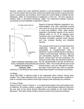
Doerr, S. H., R. A. Shakesby, and RPD Walsh. "Soil water repellency: its causes,
characteristics and hydro­geomorphological significance." ​Earth­Science
Reviews​ 51.1 (2000): 33­65.
Dale, Virginia H., et al. "Climate change and forest disturbances: climate change can
affect forests by altering the frequency, intensity, duration, and timing of fire,
drought, introduced species, insect and pathogen outbreaks, hurricanes,
windstorms, ice storms, or landslides." ​BioScience​ 51.9 (2001): 723­734.
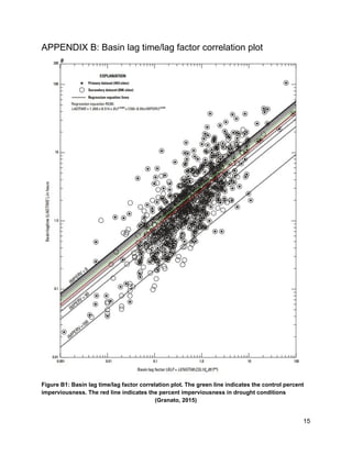
Granato, G. E. “Estimating Basin Lagtime and Hydrograph Timing Indexes Used to
Characterize Stormflows for Runoff­Quality Analysis.” Reston, Virginia. 2012.
USGS. Web.
Honarbakhsh, Afshin, Seyed Javad Sadatinejad, Moslem Heydari, and Mohamadreza
Mozdianfard. "Lag Time Forecasting in a River Basin." ​Environmental Sciences
9.1 (2012): 47. Web. 6 Dec. 2015.
Johnson, A. I. ​A Field Method for Measurement of Infiltration​. Washington, D.C.: U.S.
G.P.O., 1963. USGS. Web.
Liddell, Tommy. “Ventura County Watershed Protection District Planning & Regulatory
Hydrology Section Memorandum.” (2010). Web.
Mann, Michael E., and Peter H. Gleick. "Climate change and California drought in the
21st century." ​Proceedings of the National Academy of Sciences 112.13 (2015):
3858­3859.
"RMA Links." ​Ventura County Planning Division​. Web. 2 Dec. 2015. ­ Zoning figure
Shakesby, R. A., S. H. Doerr, and R. P. D. Walsh. "The erosional impact of soil
hydrophobicity: current problems and future research directions." ​Journal of
hydrology​ 231 (2000): 178­191.
Ventura County Watershed Protection District. "VCWPD Hydrologic Data Server."
(Hydrodata)​. Web. 7 Dec. 2015.
Wallis, M. G., D. J. Horne, and A. S. Palmer. "Water repellency in a New Zealand
development sequence of yellow brown sands." ​Soil Research 31.5 (1993):
641­654.
Walter, Lorraine. “Ventura River Watershed Management Plan.” (2015). Ventura River
Watershed Council. Web. 5 Dec. 2015.
10

12. APPENDIX A: HEC­HMS output tables
Figure A1: HEC­HMS outputs for the 2 year storm event under control conditions
Figure A2: HEC­HMS outputs for the 10 year storm event under control conditions
11

13.
Figure A3: HEC­HMS outputs for the 25 year storm event under control conditions
Figure A4: HEC­HMS outputs for the 100 year storm event under control conditions
12

14.
Figure A5: HEC­HMS outputs for the 2 year storm event under drought conditions
Figure A6: HEC­HMS outputs for the 10 year storm event under drought conditions
13

15.
Figure A7: HEC­HMS outputs for the 25 year storm event under drought conditions
Figure A8: HEC­HMS outputs for the 100 year storm event under drought conditions
14

16. APPENDIX B: Basin lag time/lag factor correlation plot
Figure B1: Basin lag time/lag factor correlation plot. The green line indicates the control percent
imperviousness. The red line indicates the percent imperviousness in drought conditions
(Granato, 2015)
15

17. APPENDIX C: Example Calculations
Weighted rainfall depth:
eighted Depth for n basins W =
i∑
n
i
A
(Ai Di)∑
n
i
*
Example for 2 year return period:
eighted Depth W = Aventura + Acalleguas + Asanta clara
Aventura Dventura + Acalleguas Dcalleguas + Asanta clara Dsanta clara * * *
eighted Depth .24 in W = 226 sqmi + 343 sqmi + 1634 sqmi
226 sqmi 3.00 in + 343 sqmi 2.44 in + 1634 sqmi 3.37 in* * *
= 3
Routing lag time:
L 0.0109LT = 0.63651
Example for Upper Ventura Reach:
L 0.0109(12, 00 m) 4.30 hours T = 0 0.63651
=
16

18. APPENDIX D: Aerial basin map
Figure D1: aerial view of the basins of study throughout Ventura County enclosed in red ­
rendered from ArcMAP 10.3.1.
17