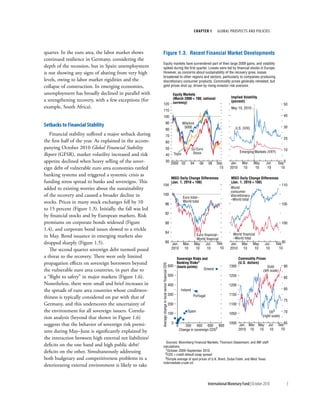
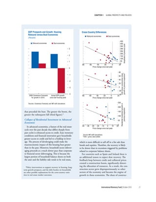
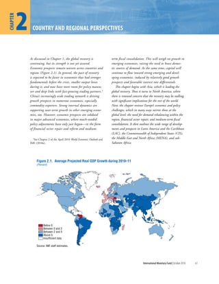
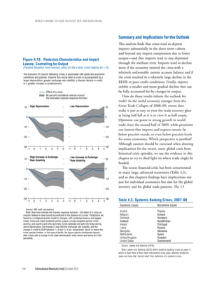
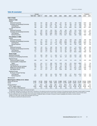
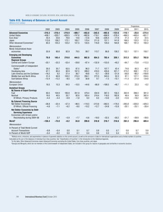
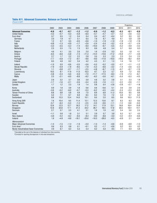
The document is the October 2010 publication of the World Economic Outlook from the International Monetary Fund. It provides an analysis of the global economic outlook and forecasts for GDP growth and inflation. The recovery from the financial crisis is ongoing but uneven across countries. Risks to the outlook include weak bank balance sheets, high unemployment, and global imbalances. More proactive fiscal and monetary policies are needed to support the recovery and rebalancing of growth.

1. World Economic and Financial Surveys
World Economic outlook
october 2010
Recovery, Risk, and Rebalancing
International Monetary Fund

2. ©2010 International Monetary Fund
Production: IMF Multimedia Services Division
Cover and Design: Luisa Menjivar and Jorge Salazar
Composition: Maryland Composition
Cataloging-in-Publication Data
World economic outlook (International Monetary Fund)
World economic outlook : a survey by the staff of the International Monetary Fund. —
Washington, DC : International Monetary Fund, 1980–
v. ; 28 cm. — (1981–1984: Occasional paper / International Monetary Fund, 0251-6365).
— (1986– : World economic and financial surveys, 0256-6877)
Semiannual. Some issues also have thematic titles.
Has occasional updates, 1984–
1. Economic development — Periodicals. 2. Economic forecasting — Periodicals.
3. Economic policy — Periodicals. 4. International economic relations —
Periodicals. I. International Monetary Fund. II. Series: Occasional paper (International
Monetary Fund). III. Series: World economic and financial surveys.
HC10.W7979
ISBN 978-1-58906-915-2
Please send orders to:
International Monetary Fund, Publication Services
P.O. Box 92780, Washington, D.C. 20090, U.S.A.
Tel.: (202) 623-7430 Fax: (202) 623-7201
E-mail: publications@imf.org
www.imfbookstore.org

3. ContEntS
Assumptions and Conventions ix
Preface xi
Foreword xiii
Executive Summary xv
Chapter 1. Global Prospects and Policies 1
Stronger Activity, but Setbacks to Financial Stability 1
Questions about the Pace of Recovery 8
More Proactive Policies Are Needed 35
Appendix 1.1. Commodity Market Developments and Prospects 45
Appendix 1.2. Indicators for Tracking Growth 55
References 59
Chapter 2. Country and Regional Perspectives 61
Asia Is Advancing with Resilience 62
The U.S. Recovery Is Moderating in the Face of Debt and Continued Uncertainty 68
Europe Is Facing a Gradual and Uneven Recovery 72
Latin America Is Sustaining Its Growth Momentum 77
The CIS Region Is Experiencing a Modest Recovery 81
The Middle East and North Africa Region Is Recovering Strongly 84
Africa’s Growth Is Accelerating 88
References 91
Chapter 3. Will It Hurt? Macroeconomic Effects of Fiscal Consolidation 93
Looking At History: What Is the Short-Term Impact of Fiscal Consolidation? 95
Additional Insights from Model Simulations 108
Lessons for Countries Considering Fiscal Consolidation 113
Appendix 3.1. Data Sources 113
Appendix 3.2. Estimation Approach 115
Appendix 3.3. Identifying Periods of Fiscal Consolidation: The Standard Approach
versus the Action-Based Approach 117
References 122
iii

4. contents
Chapter 4. Do Financial Crises Have Lasting Effects on trade? 125
Has Trade Recovered? 127
Trade Dynamics following Previous Crises 132
What Factors Are Associated with Postcrisis Import Dynamics? 139
Summary and Implications for the Outlook 144
Appendix 4.1. Data Sources 148
Appendix 4.2. Methodology and Robustness Tests 151
References 158
Annex: IMF Executive Board Discussion of the outlook, September 2010 161
Statistical Appendix 163
Assumptions 163
What’s New 168
Data and Conventions 168
Classification of Countries 169
General Features and Composition of Groups in the World Economic Outlook Classification 169
Emerging and Developing Economies 171
List of Tables 175
Output (Tables A1–A4) 177
Inflation (Tables A5–A7) 185
Financial Policies (Table A8) 191
Foreign Trade (Table A9) 192
Current Account Transactions (Tables A10–A12) 194
Balance of Payments and External Financing (Tables A13–A15) 200
Flow of Funds (Table A16) 204
Medium-Term Baseline Scenario (Table A17) 208
World Economic Outlook, Selected topics 209
Boxes
Box 1.1. Does Slow Growth in Advanced Economies Necessarily Imply Slow Growth in Emerging
Economies? 13
Box 1.2. Dismal Prospects for the Real Estate Sector 20
Box 1.3. Inferring Potential Output from Noisy Data: The Global Projection Model View 30
Box 1.4. Uncoordinated Rebalancing 41
Box 1.5. Have Metals Become More Scarce, and What Does Scarcity Mean for Prices? 51
Box 2.1. Emerging Asia: Responding to Capital Inflows 67
Box 2.2. Latin America-5: Riding Another Wave of Capital Inflows 81
Box 4.1. The Role of the Composition Effect and Intermediate Goods in the Great Trade Collapse 129
Box 4.2. Protectionism in the Recent Crisis 146
A1. Economic Policy Assumptions Underlying the Projections for Selected Economies 164
tables
Table 1.1. Overview of the World Economic Outlook Projections 2
Table 1.2. Global Oil Demand and Production by Region 48
Table 1.3. Data Summary and Model Evaluation 58
iv

5. contents
Table 2.1. Selected Asian Economies: Real GDP, Consumer Prices, Current Account Balance, and
Unemployment 64
Table 2.2. Selected Advanced Economies: Real GDP, Consumer Prices, Current Account Balance, and
Unemployment 70
Table 2.3. Selected European Economies: Real GDP, Consumer Prices, Current Account Balance, and
Unemployment 75
Table 2.4. Selected Western Hemisphere Economies: Real GDP, Consumer Prices, Current Account
Balance, and Unemployment 80
Table 2.5. Commonwealth of Independent States: Real GDP, Consumer Prices, Current Account
Balance, and Unemployment 84
Table 2.6. Selected Middle East and North African Economies: Real GDP, Consumer Prices, Current
Account Balance, and Unemployment 87
Table 2.7. Selected Sub-Saharan African Economies: Real GDP, Consumer Prices, Current Account
Balance, and Unemployment 90
Table 3.1. Long-Term Effects of a Permanent 10 Percentage Point Decrease in the G3 Government-
Debt-to-GDP Ratio: Global Integrated Monetary and Fiscal Model Simulations 112
Table 3.2. Data Sources 114
Table 3.3. Action-Based Approach: Episodes of Small Fiscal Contraction 114
Table 3.4. Action-Based Approach: Episodes of Large Fiscal Contraction 115
Table 3.5. Large Fiscal Contraction Episodes Identified by Alesina and Ardagna (2010) 115
Table 4.1. Baseline Regressions and Implied Changes in the Levels of Imports and Exports 135
Table 4.2. Estimated Elasticity of Imports 141
Table 4.3. Systemic Banking Crises, 2007–09 144
Table 4.4. Data Sources 149
Table 4.5. Country Groupings 150
Table 4.6. Unconditional Import Losses: Estimated Impulse Response Functions Using Alternative
Methodologies 152
Table 4.7. Estimated Elasticity of Imports to Output: Panel Regression with Country and Time
Dummies 153
Table 4.8. Conditional Import Losses: Robustness of Estimated Impulse Response Functions 154
Table 4.9. Import Losses and Composition Effects 157
Figures
Figure 1.1. Current and Forward-Looking Indicators 3
Figure 1.2. Global Indicators 4
Figure 1.3. Recent Financial Market Developments 5
Figure 1.4. Developments in Mature Credit Markets 6
Figure 1.5. Emerging Market Conditions 7
Figure 1.6. Public Sector Financing 8
Figure 1.7. External Developments 9
Figure 1.8. Prospects for Near-Term Activity 10
Figure 1.9. Recovery Dynamics 11
Figure 1.10. Balance Sheets and Saving Rates 12
Figure 1.11. Measures of Monetary Policy and Liquidity in Selected Advanced Economies 16
Figure 1.12. General Government Fiscal Balances and Public Debt 18
Figure 1.13. Global Outlook 19
Figure 1.14. Global Inflation 25
v

6. contents
Figure 1.15. Risks to the Global Outlook 26
Figure 1.16. Inflation, Deflation Risk, and Unemployment 27
Figure 1.17. Global Imbalances 29
Figure 1.18. Medium-Term Fiscal Policies 38
Figure 1.19. Commodity and Petroleum Prices 46
Figure 1.20. World Energy Market Developments 49
Figure 1.21. Developments in Base Metal Markets 54
Figure 1.22. Recent Developments in Markets for Major Food Crops 55
Figure 1.23. Growth Tracker 56
Figure 1.24. Stylized Example Illustrating Heat Map Colors 57
Figure 2.1. Average Projected Real GDP Growth during 2010–11 61
Figure 2.2. Asia: Average Projected Real GDP Growth during 2010–11 62
Figure 2.3. Asia: Leading the Global Recovery 63
Figure 2.4. United States and Canada: Differing Fortunes 69
Figure 2.5. United States and Canada: Average Projected Real GDP Growth during 2010–11 71
Figure 2.6. Europe: Average Projected Real GDP Growth during 2010–11 73
Figure 2.7. Europe: A Gradual and Uneven Recovery 74
Figure 2.8. Latin America and the Caribbean: Average Projected Real GDP Growth during 2010–11 78
Figure 2.9. Latin America and the Caribbean (LAC): Advancing with Strength 79
Figure 2.10. Commonwealth of Independent States: Average Projected
Real GDP Growth during 2010–11 82
Figure 2.11. Commonwealth of Independent States (CIS): A Modest Recovery 83
Figure 2.12. Middle East and North Africa: Average Projected
Real GDP Growth during 2010–11 85
Figure 2.13. Middle East and North Africa (MENA): Recovering Strongly 86
Figure 2.14. Sub-Saharan Africa: Average Projected Real GDP Growth during 2010–11 88
Figure 2.15. Sub-Saharan Africa (SSA): Growth is Accelerating 89
Figure 3.1. Action-Based Fiscal Consolidation 98
Figure 3.2. Impact of a 1 Percent of GDP Fiscal Consolidation on GDP and Unemployment 99
Figure 3.3. Response of Monetary Conditions to a 1 Percent of GDP Fiscal Consolidation 100
Figure 3.4. Impact of a 1 Percent of GDP Fiscal Consolidation on GDP Components 101
Figure 3.5. Impact of a 1 Percent of GDP Fiscal Consolidation: Taxes versus Spending 103
Figure 3.6. Composition and Monetary Conditions: Impact of a 1 Percent of
GDP Fiscal Consolidation 104
Figure 3.7. Composition and Monetary Conditions: Impact of a 1 Percent of
GDP Fiscal Consolidation 105
Figure 3.8. Impact on GDP of a 1 Percent of GDP Spending-Based Consolidation 106
Figure 3.9. Estimated Impact on GDP of a 1 Percent of GDP Fiscal Consolidation 107
Figure 3.10. Impact of Large Fiscal Consolidation on GDP and Unemployment:
Action-Based Approach versus Standard Approach 108
Figure 3.11. Impact of a 1 Percent of GDP Fiscal Consolidation: GIMF Simulations 110
Figure 3.12. Impact of a 1 Percent of GDP Fiscal Consolidation: GIMF Simulations 111
Figure 3.13. Robustness: Impact on GDP of a 1 Percent of GDP Fiscal Consolidation 116
Figure 3.14. Robustness: Impact on GDP of a 1 Percent of GDP Fiscal Consolidation 117
Figure 3.15. Size of Fiscal Consolidation: Action-Based Approach versus Standard Approach 118
Figure 4.1. The Great Trade Collapse 126
Figure 4.2. The Recovery in Trade 128
vi

7. contents
Figure 4.3. Trade Dynamics in Different Product Groups 132
Figure 4.4. Import and Export Losses, Not Controlling for Output 134
Figure 4.5. Import and Export Losses, Controlling for Output 136
Figure 4.6. Import Losses in Different Product Groups, Controlling for Output 137
Figure 4.7. Import Losses and Production Linkages, Controlling for Output 138
Figure 4.8. Trade Losses during Global Downturns 139
Figure 4.9. Precrisis Characteristics and Import Losses, Controlling for Output 140
Figure 4.10. The Postcrisis Evolution of Various Mechanisms 141
Figure 4.11. Decomposition of Import Losses 142
Figure 4.12. Import Losses and Composition Effects 143
Figure 4.13. Postcrisis Characteristics and Import Losses, Controlling for Output 144
Figure 4.14. Import Losses, Not Controlling for Output: Alternative Methodologies 153
Figure 4.15. Import Losses, Controlling for Output: Robustness 155
Figure 4.16. The Postcrisis Evolution of Various Components of GDP 156
vii

9. ASSuMPtIonS AnD ConvEntIonS
A number of assumptions have been adopted for the projections presented in the World Economic Outlook.
It has been assumed that real effective exchange rates remained constant at their average levels during August
4–September 1, 2010, except for the currencies participating in the European exchange rate mechanism II
(ERM II), which are assumed to have remained constant in nominal terms relative to the euro; that estab-
lished policies of national authorities will be maintained (for specific assumptions about fiscal and monetary
policies for selected economies, see Box A1); that the average price of oil will be $76.20 a barrel in 2010 and
$78.75 a barrel in 2011 and will remain unchanged in real terms over the medium term; that the six-month
London interbank offered rate (LIBOR) on U.S. dollar deposits will average 0.6 percent in 2010 and 0.8
percent in 2011; that the three-month euro deposit rate will average 0.8 percent in 2010 and 1.0 percent in
2011; and that the six-month Japanese yen deposit rate will yield on average 0.6 percent in 2010 and 0.4 per-
cent in 2011. These are, of course, working hypotheses rather than forecasts, and the uncertainties surround-
ing them add to the margin of error that would in any event be involved in the projections. The estimates and
projections are based on statistical information available through late September 2010.
The following conventions are used throughout the World Economic Outlook:
... to indicate that data are not available or not applicable;
– between years or months (for example, 2009–10 or January–June) to indicate the years or months
covered, including the beginning and ending years or months;
/ between years or months (for example, 2009/10) to indicate a fiscal or financial year.
“Billion” means a thousand million; “trillion” means a thousand billion.
“Basis points” refer to hundredths of 1 percentage point (for example, 25 basis points are equivalent to ¼ of
1 percentage point).
In figures and tables, shaded areas indicate IMF staff projections.
If no source is listed on tables and figures, data are drawn from the World Economic Outlook (WEO)
database.
When countries are not listed alphabetically, they are ordered on the basis of economic size.
Minor discrepancies between sums of constituent figures and totals shown reflect rounding.
As used in this report, the terms “country” and “economy” do not in all cases refer to a territorial entity that
is a state as understood by international law and practice. As used here, the term also covers some territorial
entities that are not states but for which statistical data are maintained on a separate and independent basis.
Composite data are provided for various groups of countries organized according to economic characteris-
tics or region. Unless otherwise noted, country group composites represent calculations based on 90 percent or
more of the weighted group data.
The boundaries, colors, denominations, and any other information shown on the maps do not imply, on
the part of the International Monetary Fund, any judgment on the legal status of any territory or any endorse-
ment or acceptance of such boundaries.
ix

10. FuRtHER InFoRMAtIon AnD DAtA
This version of the World Economic Outlook is available in full on the IMF’s website, www.imf.org. Accom-
panying it on the website is a larger compilation of data from the WEO database than is included in the
report itself, including files containing the series most frequently requested by readers. These files may be
downloaded for use in a variety of software packages.
Inquiries about the content of the World Economic Outlook and the WEO database should be sent by mail,
forum, or fax (telephone inquiries cannot be accepted) to
World Economic Studies Division
Research Department
International Monetary Fund
700 19th Street, N.W.
Washington, D.C. 20431, U.S.A.
Forum address: www.imf.org/weoforum Fax: (202) 623-6343
x

11. PREFACE
The analysis and projections contained in the World Economic Outlook are integral elements of the IMF’s
surveillance of economic developments and policies in its member countries, of developments in international
financial markets, and of the global economic system. The survey of prospects and policies is the product
of a comprehensive interdepartmental review of world economic developments, which draws primarily on
information the IMF staff gathers through its consultations with member countries. These consultations are
carried out in particular by the IMF’s area departments—namely, the African Department, Asia and Pacific
Department, European Department, Middle East and Central Asia Department, and Western Hemisphere
Department—together with the Strategy, Policy, and Review Department; the Monetary and Capital Markets
Department; and the Fiscal Affairs Department.
The analysis in this report was coordinated in the Research Department under the general direction of
Olivier Blanchard, Economic Counsellor and Director of Research. The project was directed by Jörg Decres-
sin, Assistant Director, Research Department, and Petya Koeva Brooks, Division Chief, Research Department.
The primary contributors to this report are Abdul Abiad, Pete Devries, Rupa Duttagupta, Charles Freed-
man, Jaime Guajardo, Prakash Kannan, Douglas Laxton, Daniel Leigh, Prachi Mishra, Andrea Pescatori, Alas-
dair Scott, and Petia Topalova. Toh Kuan, Gavin Asdorian, Stephanie Denis, Angela Espiritu, Emory Oakes,
Murad Omoev, Andy Salazar, Min Kyu Song, Ercument Tulun, and Jessie Yang provided research assistance.
Saurabh Gupta, Mahnaz Hemmati, Laurent Meister, Liessel Ampie, Vladimir Bougay, Anastasia Francis,
Wendy Mak, Shamiso Mapondera, Nhu Nguyen, Pavel Pimenov, and Steve Zhang managed the database and
the computer systems. Jenita Arshad and Tita Gunio were responsible for word processing. Other contributors
include Rudolfs Bems, John Bluedorn, Philippe Bracke, Nese Erbil, Roberto Garcia-Saltos, Robert Gregory,
Thomas Helbling, Deniz Igan, Robert C. Johnson, Michael Kumhof, Prakash Loungani, Petar Manchev, Troy
Matheson, Susanna Mursula, David Reichsfeld, Shaun Roache, Jair Rodriguez, Marina Rousset, Robert J. Tet-
low, and Kei-Mu Yi. David Romer of the Research Department provided advice and encouragement. Donald
Davis was an external consultant. Kevin Clinton provided comments and suggestions. Linda Griffin Kean of
the External Relations Department edited the manuscript and coordinated the production of the publication.
The analysis has benefited from comments and suggestions by staff from other IMF departments, as well as
by Executive Directors following their discussion of the report on September 20, 2010. However, both projec-
tions and policy considerations are those of the IMF staff and should not be attributed to Executive Directors
or to their national authorities.
xi

13. FoREWoRD
A
chieving a “strong, balanced, and sus- The result is a recovery that is neither strong nor
tained world recovery”—to quote from balanced and runs the risk of not being sustained.
the goal set in Pittsburgh by the G20— For the past year or so, inventory accumulation
was never going to be easy. It requires and fiscal stimulus were driving the recovery. The
much more than just going back to business as first is coming to an end. The second is slowly
usual. It requires two fundamental and difficult being phased out. Consumption and investment
economic rebalancing acts. now have to take the lead. But in most advanced
First, internal rebalancing: When private demand economies, weak consumption and investment,
collapsed, fiscal stimulus helped alleviate the fall in together with little improvement in net exports, are
output. But fiscal stimulus has to eventually give leading to low growth. Unemployment is high and
way to fiscal consolidation, and private demand barely decreasing. By contrast, in many emerging
must be strong enough to take the lead and sustain market economies, where excesses were limited and
growth. the scars are few, consumption, investment, and net
Second, external rebalancing: Many advanced exports are all contributing to strong growth, and
economies, most notably the United States, which output is once again close to potential.
relied excessively on domestic demand, must now What can be done to improve things?
rely more on net exports. Many emerging mar- First, and wherever private demand is weak,
ket economies, most notably China, which relied central banks should continue with accommodative
excessively on net exports, must now rely more on monetary policy. However, one should be realistic.
domestic demand. Not much more can be done, and one should not
These two rebalancing acts are taking place too expect too much from further quantitative or credit
slowly. easing. While there is no evidence yet that sustained
Private domestic demand remains weak in low interest rates are leading to excessive risk tak-
advanced economies. This weakness reflects both ing, should such risks materialize, they should be
a correction of precrisis excesses and the scars of addressed through macroprudential measures, not
the crisis. U.S. consumers who had overborrowed through increases in policy rates.
before the crisis are now saving more and consum- Second, and wherever needed, governments
ing less, and while this is good for the long term, must continue both financial repair and financial
it is a drag on demand in the short term. Hous- reform. Many banks remain undercapitalized, and
ing booms have given way to housing slumps, and tight credit is constraining segments of demand.
housing investment will remain depressed for some Securitization, which must play an important role
time. And weaknesses in the financial system are in any future intermediation system, is still mori-
still constraining credit. bund. Financial reform is proceeding, but questions
External rebalancing remains limited. Net exports remain about “too-big-to-fail” institutions, the
are not contributing to growth in advanced econo- perimeter of regulation, and cross-border issues. The
mies, and the U.S. trade deficit remains large. Many faster reform uncertainty is reduced, the more the
emerging market economies continue to run large financial system will support demand and growth.
current account surpluses and to respond to capital Third, and again wherever needed, governments
inflows primarily through reserve accumulation must address fiscal consolidation. What is essential
rather than exchange rate appreciation. Interna- is not so much phasing out fiscal stimulus now,
tional reserves are higher than they have ever been but offering credible medium-term plans for debt
and continue to increase. stabilization and, eventually, debt reduction. Such
xiii

14. FoReWoRD
credible plans may involve fiscal rules, the cre- production toward domestic goods. Finally, to the
ation of independent fiscal agencies, and phased-in extent that countries remain worried about sudden
entitlement reforms. They have not been offered in stops, better provision of global liquidity can play
most countries, but they are essential and, once in an important role and limit the accumulation of
place, will give governments more fiscal flexibility to reserves.
sustain growth in the short term. All these pieces are interconnected. Unless
Fourth, emerging market economies with large advanced economies can count on stronger private
current account surpluses must accelerate rebal- demand, both domestic and foreign, they will find
ancing. This is not only in the world economy’s it difficult to achieve fiscal consolidation. And wor-
interest, but also in their own. In many coun- ries about sovereign risk can easily derail growth.
tries, distortions have led to too low a level of If growth stops in advanced economies, emerging
consumption or too little investment. Removing market economies will have a hard time decoupling.
these distortions and thus allowing consumption The need for careful design at the national level,
and investment to increase is desirable. To a large and coordination at the global level, may be even
extent, market forces in the form of large capital more important today than at the peak of the crisis,
inflows are pushing these countries in the right a year and a half ago.
direction. Unless offset by reserve accumulation,
capital inflows will lead to exchange rate apprecia-
tion. With the help of macroprudential measures Olivier Blanchard
and capital controls, these flows can help reallocate Economic Counsellor
xiv

15. ExECutIvE SuMMARy
Thus far, economic recovery is proceeding broadly as Economic Outlook (WEO) Update. A surge in inven-
expected, but downside risks remain elevated. Most tory and, lately, fixed investment accounted for a
advanced economies and a few emerging economies dramatic rise in manufacturing and global trade.
still face large adjustments. Their recoveries are Low consumer confidence and reduced household
proceeding at a sluggish pace, and high unemploy- incomes and wealth are holding consumption down
ment poses major social challenges. By contrast, many in many advanced economies. Growth in these
emerging and developing economies are again seeing economies reached only about 3½ percent during
strong growth, because they did not experience major the first half of 2010, a low rate considering that
financial excesses just prior to the Great Recession. they are emerging from the deepest recession since
Sustained, healthy recovery rests on two rebalancing World War II. Their recoveries will remain fragile
acts: internal rebalancing, with a strengthening of for as long as improving business investment does
private demand in advanced economies, allowing for not translate into higher employment growth. How-
fiscal consolidation; and external rebalancing, with ever, household spending is doing well in many
an increase in net exports in deficit countries, such emerging market economies, which expanded by
as the United States, and a decrease in net exports in close to 8 percent and where investment is propel-
surplus countries, notably emerging Asia. The two ling job creation. This heterogeneity in the pace of
interact in strong ways. Increased net exports in recovery across advanced and emerging economies
advanced economies imply higher demand and higher is discussed in detail in Chapter 2.
growth, allowing more room for fiscal consolida- At the same time, financial stability suffered a
tion. Strengthened domestic demand helps emerging major setback, as explained in the accompanying
market economies maintain growth in the face of October 2010 Global Financial Stability Report
lower exports. A number of policies are required to (GFSR). Market volatility increased and investor
support these rebalancing acts. In advanced economies, confidence dropped. Prices in many stock exchanges
the repair and reform of the financial sector need fell, led initially by financial stocks and by Euro-
to accelerate to allow a resumption of healthy credit pean markets. Heavy selling of the sovereign debt of
growth. In addition, fiscal adjustment needs to start vulnerable euro area economies rattled the bank-
in earnest in 2011. Specific plans to cut future budget ing system, triggering a systemic crisis. This added
deficits are urgently needed now to create new room to existing worries about the sustainability of the
for fiscal policy maneuver. If global growth threatens recovery and caused a broader decline in stocks.
to slow appreciably more than expected, countries Risk premiums on corporate bonds widened, and
with fiscal room could postpone some of the planned corporate bond issues slowed to a trickle in May.
consolidation. Meanwhile, key emerging economies Issuance in emerging markets also dropped sharply.
will need to further develop domestic sources of growth, Since the beginning of the summer, however, finan-
with the support of greater exchange rate flexibility. cial conditions have improved again. Tail risks have
been reduced by unprecedented European policy
initiatives—the European Central Bank’s Securi-
Stronger Activity, but Setbacks to Financial ties Markets Program and euro area governments’
Stability European Stabilization Mechanism—and by a
Economic recovery continued to strengthen dur- front-loading of fiscal adjustment. However, under-
ing the first half of 2010. Global activity expanded lying sovereign and banking vulnerabilities remain a
at an annual rate of about 5¼ percent––about ½ significant challenge amid lingering concerns about
percent higher than anticipated in the July World risks to the global recovery.
xv

16. eXecUtIVe sUMMARY
Questions about the Pace of Recovery expected, countries with fiscal room could postpone
some of the planned consolidation. One of the
The global recovery remains fragile, because
most urgent challenges for advanced economies is
strong policies to foster internal rebalancing of
to legislate plans that help achieve sustainable fiscal
demand from public to private sources and exter-
positions before the end of the decade. This task is
nal rebalancing from deficit to surplus economies
now more pressing than it was six months ago to
are not yet in place. Global activity is forecast to
rebuild room for fiscal policy maneuver in the face
expand by 4.8 percent in 2010 and 4.2 percent
of still-volatile sovereign debt markets. Such room
in 2011, broadly in line with earlier expectations,
could be needed because monetary policy alone
and downside risks continue to predominate.
might not be able to provide sufficient support to
WEO projections are that output of emerging and
counter the threat of a weakening of activity that is
developing economies will expand at rates of 7.1
markedly more pronounced than expected.
and 6.4 percent, respectively, in 2010 and 2011. In
Fiscal policy tightening will likely prove contrac-
advanced economies, however, growth is projected
tionary in most economies, although the extent is
at only 2.7 and 2.2 percent, respectively, with some
difficult to gauge. The survey of past experience
economies slowing noticeably during the second
in Chapter 3 suggests that fiscal consolidation
half of 2010 and the first half of 2011, followed
in advanced economies typically detracts from
by a reacceleration of activity. Slack will remain
short-term growth. The introduction of credible,
substantial and unemployment persistently high.
growth-friendly, medium-term fiscal consolidation
Inflation is projected to stay generally low, amid
plans––currently not on offer in many advanced
continued excess capacity and high unemployment,
economies––would help limit the deflationary
with a few exceptions among the emerging econo-
impact of consolidation on private demand in
mies. Risks to the growth forecasts are mainly to
the short term. Such plans would have to include
the downside. However, the probability of a sharp
reforms to rapidly growing spending programs,
global slowdown, including stagnation or contrac-
notably entitlements, and tax reforms that favor
tion in advanced economies, still appears low.
production rather than consumption.
Better financial sector policies and practices in
advanced economies are critical for strengthening
More Proactive Policies Are needed the resilience of the recovery to shocks and sustain-
Policies need to become more proactive to ing private demand over the medium term. Progress
achieve the required internal and external rebalanc- on this front has been very slow. Apparently isolated
ing. Most advanced economies and a few emerging difficulties in a few spots can have large spillover
economies still face major adjustments, including effects, via complex financial linkages and deterio-
the need to strengthen household balance sheets, ration of fragile confidence. As the October 2010
stabilize and subsequently reduce high public GFSR explains, incomplete progress in addressing
debt, and repair and reform their financial sectors. the legacy problems of the crisis has left systems in
Monetary policy should stay highly supportive in advanced economies vulnerable. Failure to rapidly
most of the advanced economies and should be the resolve, restructure, or consolidate weak banks and
first line of defense against any larger-than-projected repair wholesale markets raises the need for further
weakening of activity as fiscal support diminishes. fiscal backstopping and low interest rates to support
With policy rates already near zero in the large recovery, which can cause other problems, includ-
advanced economies, monetary policymakers may ing spillovers to emerging economies. More broadly,
have to resort to further unconventional measures policymakers need to continue to clarify and specify
if private demand weakens unexpectedly as fiscal regulatory reform, building on the improvements
support wanes. proposed by the Basel Committee on Banking
Fiscal adjustment needs to start in 2011. If global Supervision. This would help financial markets and
growth threatens to slow appreciably more than institutions provide more support, on a sounder
xvi

17. eXecUtIVe sUMMARY
basis, for consumption and investment, which is immediately, because domestic demand recovery is
essential for strong, sustainable growth. already well under way or public debt is relatively
Structural policies that strengthen growth over high. In various emerging economies, rising infla-
the medium term would also help support the tion or high credit growth also signal a need for
required normalization of macroeconomic policies further monetary tightening.
in advanced economies. While supportive macro- Many emerging and developing economies have
economic policies and financial sector repair and successfully concluded first-generation reforms
reform are essential for stronger job creation, in a that improved macroeconomic policy frameworks,
number of economies, labor market policies could strengthening their resilience to macroeconomic
enhance growth and job creation and reduce high shocks. However, to sustain or further raise poten-
unemployment over the medium term. Comple- tial growth and employment, efforts could usefully
mentary reforms to product and services markets focus on simplifying product and services market
could strengthen the employment effects by boost- regulation, raising human capital, and building
ing labor demand and real wages through greater critical infrastructure. Such reforms would also help
competition and lower markups on prices. absorb growing capital inflows in a productive man-
Although many emerging economies are seeing ner, which would accelerate global income conver-
high growth again, they continue to rely sig- gence and external rebalancing. As Chapter 1 and
nificantly on demand from advanced economies. the October 2010 GFSR underscore, these flows
Chapter 4 makes clear that demand for imports can be expected to grow over the medium term, as
from the advanced economies will continue to be the performance of emerging economies improves
below precrisis trends, in view of the high share relative to that of the advanced economies, yields in
of consumer durables and investment goods in the advanced economies remain low for some time,
trade. Emerging economies that relied heavily on and institutional investors in advanced economies
demand from these economies will therefore have to continue to diversify their exposures.
rebalance growth further toward domestic sources Strong, coordinated policy responses by all are
to achieve growth rates similar to those before the essential to limit the fallout of the Great Reces-
crisis, helping the required external rebalancing. sion. Historical evidence suggests that countries
In economies with excessive external surpluses, hit by financial crises typically suffer permanent
which are mainly in emerging Asia, fiscal tighten- output losses relative to precrisis trends. How-
ing should therefore take a backseat to monetary ever, outcomes after individual crises have varied
tightening and exchange rate flexibility. Removing widely, depending on the policy responses. So far,
distortions that drive high household or corporate much progress has been made through coordinated
saving rates and deter investment in nontradables policy responses in alleviating liquidity strains and
sectors would facilitate the rebalancing of growth rebuilding confidence, and this has been essential
to domestic sources. Such rebalancing will require for activity to rebound. The challenge ahead is for
further deregulation and reform of financial sectors policymakers to put in place, in a coordinated man-
and corporate governance, as well as stronger social ner, policies that support the fundamental adjust-
safety nets in key Asian economies. In many other ments needed for a return to healthy medium-term
emerging economies, fiscal tightening can start growth.
xvii

19. 1
chapter
Global proSpectS and policieS
Thus far, economic recovery is proceeding broadly as solidation. Meanwhile, key emerging economies will
expected, although downside risks remain elevated. Most need to further develop domestic sources of growth,
advanced and a few emerging economies still face major with the support of greater exchange rate flexibility.
adjustments, including the need to strengthen household
balance sheets, stabilize and subsequently reduce high
public debt, and repair and reform their financial sectors. Stronger activity, but Setbacks to Financial
In many of these economies, the financial sector is still Stability
vulnerable to shocks, and growth appears to be slow- Economic recovery continued to strengthen
ing as policy stimulus wanes. By contrast, in emerging during the first half of 2010, but global financial
and developing economies prudent policies, implemented stability suffered a major setback with the turmoil
partly in response to earlier crises, have contributed to in sovereign debt markets in the second quarter
a significantly improved medium-term growth outlook of 2010. The extent of economic recovery differs
relative to the aftermath of previous global recessions. importantly across regions, with Asia in the lead.
However, activity in these economies, particularly those The United States and Japan experienced a notice-
in emerging Asia, remains dependent on demand in able slowdown during the second quarter of 2010,
advanced economies. In this setting, global activity is fore- while growth accelerated in Europe and stayed
cast to expand by 4.8 percent in 2010 and 4.2 percent in strong in emerging and developing economies.
2011, with a temporary slowdown during the second half Financial conditions have begun to normalize, but
of 2010 and the first half of 2011. Output of emerg- institutions and markets are still fragile. In general,
ing and developing economies is projected to expand at volatility in financial, currency, and commodity
rates of 7.1 percent and 6.4 percent in 2010 and 2011, markets remains elevated.
respectively. In advanced economies, however, growth is
projected to be only 2.7 percent and 2.2 percent, respec-
tively. Risks to the forecast are mainly to the downside. Growing Momentum through the First half of 2010
Sustained, healthy recovery rests on two rebalancing acts: The world economy expanded at an annual rate
internal rebalancing, with a strengthening of private of about 5¼ percent during the first half of 2010––
demand in advanced economies, allowing for fiscal about ½ percent higher than in the July 2010 World
consolidation; and external rebalancing, with an increase Economic Outlook (WEO) Update (Table 1.1). World
in net exports in deficit countries and a decrease in net industrial production reached growth rates of about
exports in surplus countries, notably emerging Asia. The 15 percent, and global trade recovered at rates over
two interact in strong ways. Increased net exports in 40 percent during this period (Figure 1.1). A surge
advanced economies imply higher demand and higher in inventory and, lately, fixed investment accounts
growth, allowing more room for fiscal consolidation. A for this dramatic rise––with the latter in particular
number of policies are required to support these rebalanc- boding well for continued recovery. Manufacturing
ing acts. In advanced economies, repair and reform of the confidence indices are back to precrisis levels, and
financial sector need to accelerate to allow a resumption employment in advanced economies is expanding
of healthy credit growth. In addition, fiscal adjustment moderately. Household spending is doing well in
needs to start in earnest in 2011. Specific plans to cut emerging market economies, but in advanced econo-
future budget deficits are urgently needed to create new mies, low consumer confidence, high unemployment,
room for fiscal policy maneuver. If global growth threatens stagnant incomes, and reduced household wealth
to slow appreciably more than expected, countries with are holding consumption down. Chapter 2 discusses
fiscal room could postpone some of the planned con- regional developments in more detail.
International Monetary Fund | October 2010 1

20. wOrld ecOnOmic OutlOOk: recOvery, risk, and rebalancing
Table 1.1. Overview of the World Economic Outlook Projections
(Percent change, unless noted otherwise)
Year over Year
Difference from July Q4 over Q4
Projections 2010 WEO Projections Estimate Projections
2008 2009 2010 2011 2010 2011 2009 2010 2011
World Output1 2.8 –0.6 4.8 4.2 0.2 –0.1 2.0 4.3 4.4
Advanced Economies 0.2 –3.2 2.7 2.2 0.1 –0.2 –0.4 2.4 2.5
United States 0.0 –2.6 2.6 2.3 –0.7 –0.6 0.2 2.2 2.7
Euro Area 0.5 –4.1 1.7 1.5 0.7 0.2 –2.0 1.9 1.4
Germany 1.0 –4.7 3.3 2.0 1.9 0.4 –2.0 3.9 1.2
France 0.1 –2.5 1.6 1.6 0.2 0.0 –0.5 1.7 1.6
Italy –1.3 –5.0 1.0 1.0 0.1 –0.1 –2.8 1.3 1.1
Spain 0.9 –3.7 –0.3 0.7 0.1 0.1 –3.0 0.1 1.4
Japan –1.2 –5.2 2.8 1.5 0.4 –0.3 –1.4 1.9 2.1
United Kingdom –0.1 –4.9 1.7 2.0 0.5 –0.1 –2.9 2.8 1.6
Canada 0.5 –2.5 3.1 2.7 –0.5 –0.1 –1.1 3.1 2.9
Other Advanced Economies 1.7 –1.2 5.4 3.7 0.8 –0.0 3.2 4.2 4.7
Newly Industrialized Asian Economies 1.8 –0.9 7.8 4.5 1.1 –0.2 6.1 5.2 6.6
Emerging and Developing Economies2 6.0 2.5 7.1 6.4 0.3 0.0 5.6 7.0 7.0
Central and Eastern Europe 3.0 –3.6 3.7 3.1 0.5 –0.3 1.8 2.9 4.3
Commonwealth of Independent States 5.3 –6.5 4.3 4.6 0.0 0.3 –3.2 3.3 5.0
Russia 5.2 –7.9 4.0 4.3 –0.3 0.2 –2.9 3.2 5.0
Excluding Russia 5.4 –3.2 5.3 5.2 0.9 0.5 ... ... ...
Developing Asia 7.7 6.9 9.4 8.4 0.2 –0.1 9.5 9.1 8.7
China 9.6 9.1 10.5 9.6 0.0 0.0 11.4 9.9 9.6
India 6.4 5.7 9.7 8.4 0.3 0.0 7.3 10.3 7.9
ASEAN-53 4.7 1.7 6.6 5.4 0.2 –0.1 5.1 5.0 6.8
Latin America and the Caribbean 4.3 –1.7 5.7 4.0 0.9 0.0 1.4 4.8 4.4
Brazil 5.1 –0.2 7.5 4.1 0.4 –0.1 4.4 5.6 4.5
Mexico 1.5 –6.5 5.0 3.9 0.5 –0.5 –2.3 3.1 4.5
Middle East and North Africa 5.0 2.0 4.1 5.1 –0.4 0.2 ... ... ...
Sub-Saharan Africa 5.5 2.6 5.0 5.5 0.0 –0.4 ... ... ...
Memorandum
European Union 0.8 –4.1 1.7 1.7 0.7 0.1 –2.1 2.1 1.7
World Growth Based on Market Exchange Rates 1.6 –2.0 3.7 3.3 0.1 –0.1 ... ... ...
World Trade Volume (goods and services) 2.9 –11.0 11.4 7.0 2.4 0.7 ... ... ...
Imports
Advanced Economies 0.4 –12.7 10.1 5.2 2.9 0.6 ... ... ...
Emerging and Developing Economies 9.0 –8.2 14.3 9.9 1.8 0.6 ... ... ...
Exports
Advanced Economies 1.9 –12.4 11.0 6.0 2.8 1.0 ... ... ...
Emerging and Developing Economies 4.6 –7.8 11.9 9.1 1.4 0.1 ... ... ...
Commodity Prices (U.S. dollars)
Oil4 36.4 –36.3 23.3 3.3 1.5 0.3 ... ... ...
Nonfuel (average based on world
commodity export weights) 7.5 –18.7 16.8 –2.0 –1.3 –0.6 ... ... ...
Consumer Prices
Advanced Economies 3.4 0.1 1.4 1.3 0.0 0.0 0.8 1.1 1.6
Emerging and Developing Economies2 9.2 5.2 6.2 5.2 –0.1 0.2 4.8 5.9 4.4
London Interbank Offered Rate (percent)5
On U.S. Dollar Deposits 3.0 1.1 0.6 0.8 0.0 –0.1 ... ... ...
On Euro Deposits 4.6 1.2 0.8 1.0 0.0 –0.2 ... ... ...
On Japanese Yen Deposits 1.0 0.7 0.6 0.4 0.1 –0.2 ... ... ...
Note: Real effective exchange rates are assumed to remain constant at the levels prevailing during August 4–September 1, 2010. Country weights used to construct aggregate growth rates for groups
of economies were revised. When economies are not listed alphabetically, they are ordered on the basis of economic size. The aggregated quarterly data are seasonally adjusted.
1The quarterly estimates and projections account for 90 percent of the world purchasing-power-parity weights.
2The quarterly estimates and projections account for approximately 78 percent of the emerging and developing economies.
3Indonesia, Malaysia, Philippines, Thailand, and Vietnam.
4Simple average of prices of U.K. Brent, Dubai, and West Texas Intermediate crude oil. The average price of oil in U.S. dollars a barrel was $61.78 in 2009; the assumed price based on futures
markets is $76.20 in 2010 and $78.75 in 2011.
5Six-month rate for the United States and Japan. Three-month rate for the euro area.
2 International Monetary Fund | October 2010

21. chapter 1 Global ProsPects and PolIcIes
Growth in advanced economies reached about Figure 1.1. Current and Forward-Looking Indicators1
3½ percent during the first half of 2010. This is (Annualized percent change of three-month moving average over previous
low, considering that these economies are emerg- three-month moving average, unless noted otherwise)
ing from the deepest recession since World War II. World trade and industrial production have continued to rebound, and
employment has begun to grow again in advanced economies. Retail sales have
Three groups can be distinguished (Figure 1.2): recovered. They are buoyant in emerging economies but lagging in advanced
• The economies of advanced Asia, other than economies, reflecting still-low consumer confidence. Recently, manufacturing
confidence has receded, but it remains consistent with further expansion.
Japan, have enjoyed a strong rebound. Their large
manufacturing sectors have benefited from the 60 World Trade Industrial Production
Emerging 30
global rebound in trade. As a result, their output 40
Asia
20
is already above precrisis levels. Trade value2
• The United States is close to precrisis levels of 20 10
output but far below precrisis trends, and activity 0 0
Emerging
slowed noticeably in the second quarter of 2010. CPB trade economies3
-20 volume index World -10
Consumption has been growing since the third Advanced
economies4
quarter of 2009, but at low rates considering the -40 -20
depth of the retrenchment. At the same time, -60 -30
2000 02 04 06 08 Jul. 2005 06 07 08 09 Jul.
investment in business equipment and software 10 10
has been rising strongly lately, helped by foreign 6 Employment Emerging Retail Sales 36
Emerging Asia
demand, rebounding profits, and normalizing economies3
4 Emerging 27
financial conditions. However, this has not yet World economies3
triggered a sustained, solid recovery in employ- 2 18
ment and real estate activity remains very weak. World
0 9
• Japan and the euro area are still appreciably
-2 Advanced 0
below precrisis levels of output and remain economies4
Advanced
dependent on foreign demand. In Japan, fiscal -4 economies4 -9
stimulus and the rebound in global trade and
-6 -18
strong demand elsewhere in Asia have boosted 2005 06 07 08 09 Jul. 2005 06 07 08 09 Jul.
10 10
output growth since the fourth quarter of 2009, Manufacturing Purchasing Consumer Confidence
but activity weakened significantly in the second 65 Managers’ Index 180 (index) 5
(index) Emerging
quarter of 2010. In the euro area, led by Ger- 60 160 0
economies3
Euro area
many, activity showed significant strength only 140 (right scale) -5
55
in the second quarter of this year, following 50
120 -10
a bad winter. The area’s dependence on bank Advanced
100 -15
45 economies4
credit is restraining demand, as banks continue 80 United -20
40 States
to be unusually cautious in lending. However, 60 Japan5 (left scale) -25
(left scale)
the depreciation of the euro from previous highs 35 40 -30
is beginning to support the euro area’s tradable 30
2000 02 04 06 08 Aug.
20
2000 02 04 06
-35
08 Aug.
goods sector, and fixed investment is staging a 10 10
modest comeback. Sources: Netherlands Bureau for Economic Policy Analysis for CPB trade volume index;
for all others, Haver Analytics and NTC Economics; and IMF staff calculations.
Emerging economies expanded by about 8 per- 1Not all economies are included in the regional aggregations. For some economies,
cent during the first half of the year. As in advanced monthly data are interpolated from quarterly series.
2In SDR terms.
economies, there is significant heterogeneity both 3Argentina, Brazil, Bulgaria, Chile, China, Colombia, Estonia, Hungary, India, Indonesia,
Latvia, Lithuania, Malaysia, Mexico, Pakistan, Peru, Philippines, Poland, Romania, Russia,
across and within regions, with Asian and Latin South Africa, Thailand, Turkey, Ukraine, and Venezuela.
4Australia, Canada, Czech Republic, Denmark, euro area, Hong Kong SAR, Israel, Japan,
American economies in the lead. In both regions,
Korea, New Zealand, Norway, Singapore, Sweden, Switzerland, Taiwan Province of
fixed investment has expanded vigorously, just as China, United Kingdom, and United States.
5Japan’s consumer confidence data are based on a diffusion index, where values
inventory rebuilding has slowed and policy stimulus greater than 50 indicate improving confidence.
has waned. This is a sign that autonomous private
International Monetary Fund | October 2010 3

22. wOrld ecOnOmic OutlOOk: recOvery, risk, and rebalancing
Figure 1.2. Global Indicators1 demand is overtaking short-term, policy-related fac-
(Annual percent change, unless noted otherwise) tors in the recovery.
Private consumption has recovered impressively in emerging economies but is
• Growth in emerging Asia reached about 9½
lagging in advanced economies. However, investment excluding construction percent, as robust domestic demand spread from
has staged a rebound in advanced economies, suggesting medium- rather than
short-term considerations are increasingly driving activity. This bodes well for China, India, and Indonesia to other Asian
employment and consumption in the future. In the meantime, output in many economies. In China, major fiscal stimulus, a
advanced economies is still around or below precrisis levels. Commodity prices
have recovered. Recent wheat price hikes are not representative of broader large expansion of credit, and a number of spe-
developments in food prices. cific measures to boost household incomes and
Real Private Consumption Real Gross Fixed Investment consumption increased domestic demand growth
(annualized percent change (annualized percent change to close to 13 percent in 2009, contributing to a
12 from preceding quarter) from preceding quarter) 20
large decline in the current account surplus. The
10 recovery is now well established, and a transition
8 Emerging
economies 0 from public stimulus to private-sector-led growth
Emerging is under way.
4 -10
economies • Latin America has also recovered strongly,
Advanced -20 with real GDP growth at about 7 percent. The
0 economies
Advanced -30 recovery is being led by Brazil, where real GDP
economies of which:
machinery and equipment2 growth has been running close to 10 percent
-4 -40
2007: 08: 09: 10: 2007: 08: 09: 10: since the third quarter of 2009 and the economy
Q1 Q1 Q1 Q2 Q1 Q1 Q1 Q2
is now showing signs of overheating. A number
125 Change in GDP3 Real Commodity Prices 500
(2010:Q2 GDP in percent of (1995 = 100) of other economies have also returned to solid
120 2008:Q2 GDP)
400 growth. However, Mexico is lagging, partly
115
because of its strong trade linkages with the
Oil prices4 300
110 United States. Growth in Mexico recently picked
Gold
105 200 up on the back of strengthening exports to the
100 United States, but the output gap remains large.
95 Food
100 • Many developing economies were less affected by
Metals
the global recession and now seem to be shar-
90 0
US/EA EAS LA CEE AFR and 1980 85 90 95 2000 05 10 15 ing in the pickup in world trade, and estimates
JP/OAAE and CIS ME
for growth in 2010 are generally encouraging.
Output since Trough for Highly Synchronized Recessions
(Index; quarters from trough on x-axis) Available data for African and Middle Eastern
114 United States Euro Area 114
economies point to robust growth. By contrast,
112 112
1975:Q1 1975:Q1 economies that were hit particularly hard by the
110 1982:Q3 1982:Q3 110
1991:Q1 1993:Q1 crisis are struggling to return to sustained growth,
108 2009:Q2 2009:Q2 108 including in many parts of emerging Europe and
106 106 the Commonwealth of Independent States, where
104 104 the recovery remains much more subdued.
102 102 Unemployment in advanced economies has
100 100 receded only modestly from peak rates. Estimates
98 98 are that more than 210 million people across the
-4 -2 0 2 4 6 8 -4 -2 0 2 4 6 8
Source: IMF staff estimates. globe are unemployed, an increase of more than 30
1Aggregates are computed on the basis of purchasing-power-parity (PPP) weights,
unless noted otherwise.
million since 2007. Three-fourths of the increase
2PPP-weighted averages of metal products and machinery for euro area, plants and has occurred in the advanced economies (with the
equipment for Japan, plants and machinery for the United Kingdom, and equipment and
software for the United States. remainder in emerging market economies). In the
3US/EA/JP/OAAE: United States/euro area/Japan/other advanced Asian economies;
EAS: emerging Asia; LA: Latin America; CEE and CIS: central and eastern Europe and
United States, the unemployed face record-long
Commonwealth of Independent States; AFR and ME: Africa and Middle East. periods of joblessness, and recent payroll data point
4Simple average of spot prices of U.K. Brent, Dubai Fateh, and West Texas
Intermediate crude oil. to a slowdown in employment growth in the second
4 International Monetary Fund | October 2010

23. chapter 1 Global ProsPects and PolIcIes
quarter. In the euro area, the labor market shows Figure 1.3. Recent Financial Market Developments
continued resilience in Germany, considering the
Equity markets have surrendered part of their large 2009 gains, and volatility
depth of the recession, but in Spain unemployment spiked during the first quarter. Losses were led by financial stocks in Europe.
is not showing any signs of abating from very high However, as concerns about sustainability of the recovery grew, losses
broadened to other regions and sectors, particularly to companies producing
levels, owing to labor market rigidities and the discretionary consumer products. Commodity prices generally retreated, but
collapse of construction. In emerging economies, gold prices shot up, driven by rising investor risk aversion.
unemployment has broadly declined in parallel with Equity Markets
(March 2000 = 100; national Implied Volatility
a strengthening recovery, with a few exceptions (for currency) (percent)
120 50
example, South Africa). May 10, 2010
110
100 40
90 Wilshire
Setbacks to Financial Stability 5000 U.S. (VIX) 30
80
Financial stability suffered a major setback during 70
20
the first half of the year. As explained in the accom- 60
panying October 2010 Global Financial Stability 50 DJ Euro 10
Stoxx Emerging Markets (VXY)
Report (GFSR), market volatility increased and risk 40 Topix
appetite declined when heavy selling of the sover- 30
2000 02 04 06 08 Sep. Jan. Mar. May Jul. 0
Sep.
eign debt of vulnerable euro area economies rattled 10 2010 10 10 10 10
banking systems and triggered a systemic crisis as
MSCI Daily Change Differences MSCI Daily Change Differences
funding stress spread to banks and sovereigns. This (Jan. 1, 2010 = 100) (Jan. 1, 2010 = 100)
104 110
added to existing worries about the sustainability World
consumer
of the recovery and caused a broader decline in 100
Euro total–
discretionary
–World total
stocks. Prices in many stock exchanges fell by 10 96
World total
105
to 15 percent (Figure 1.3). Initially, the fall was led
92
by financial stocks and by European markets. Risk
premiums on corporate bonds widened (Figure 88 100
1.4), and corporate bond issues slowed to a trickle
84 World financial
in May. Bond issuance in emerging markets also Euro financial–
World financial –World total
dropped sharply (Figure 1.5). 80 Jan. Mar. May Jul. Sep. Jan. Mar. May Jul. Sep.95
2010 10 10 10 10 2010 10 10 10 10
The second quarter sovereign debt turmoil posed
a threat to the recovery. There were only limited Sovereign Risks and Commodity Prices
propagation effects on sovereign borrowers beyond Banking Risks1 (U.S. dollars)
Average change in local senior financial CDS
600 (basis points) 1300 Gold 90
the vulnerable euro area countries, in part due to Greece (left scale)
a “flight to safety” in major markets (Figure 1.6). 500 1250
85
Nonetheless, there were small and brief increases in 400 1200
the spreads of euro area countries whose creditwor- Ireland 80
300 Portugal 1150
thiness is typically considered on par with that of
75
Germany, and this underscores the uncertainty of 200 1100
the environment for all sovereign issuers. Correla- 100
Spain
1050 Oil3 70
(right scale)
tion analysis (beyond that shown in Figure 1.6)
suggests that the behavior of sovereign risk premi- 0 1000 65
Sep.
0 200 400 600 800 Jan. Mar. May Jul.
ums during May–June is significantly explained by Change in sovereign CDS2 2010 10 10 10 10
the interaction between high external net liabilities/
Sources: Bloomberg Financial Markets; Thomson Datastream; and IMF staff
deficits on the one hand and high public debt/ calculations.
1October 2009–September 2010.
deficits on the other. Simultaneously addressing 2CDS = credit default swap spread.
both budgetary and competitiveness problems in a 3Simple average of spot prices of U.K. Brent, Dubai Fateh, and West Texas
Intermediate crude oil.
deteriorating external environment is likely to take
International Monetary Fund | October 2010 5

24. wOrld ecOnOmic OutlOOk: recOvery, risk, and rebalancing
Figure 1.4. Developments in Mature Credit Markets a heavy toll on growth, which may help explain
Funding strains in advanced economy banking markets reappeared, but tensions why some euro area banking systems came under
remained much lower than one year earlier. Bond yields for Germany, Japan, and particular strain.
the United States declined amid investor flight to safe havens and rising concerns
about the sustainability of the recovery. However, yields in vulnerable euro area
countries rose because of concerns about high public and external deficits and
debt. Notwithstanding the turbulence, bank lending conditions in major there are Signs of normalization, but important
economies continued to normalize. Corporate spreads widened somewhat, and
issuance briefly dried up. Vulnerabilities remain
Interbank Spreads1 Bank CDS Spreads In recent months, financial conditions have
500 400
(basis points) (ten-year, median; in basis
points) been easing again. Tail risks have been reduced by
400
300 unprecedented European policy initiatives––the
300
U.S. United European Central Bank’s (ECB’s) Securities Markets
States
200
dollar
200
Program (SMP) and euro area governments’ Euro-
Euro
pean Stabilization Mechanism––and by a front-
100 area
100
loading of fiscal adjustment in response to market
0 pressures. However, underlying sovereign and
Yen Euro banking vulnerabilities pose a significant challenge
-100 0
2000 02 04 06 08 Sep. 2003 04 05 06 07 08 09 Sep. amid lingering concerns about risks to the global
10 10
Government Bond Yields2
Government Bond Spreads recovery.
(two-year yield spreads
6 700 over German bunds, 2000 • Sovereign bond auctions in the euro area have
United basis points) successfully rolled over substantial maturities,
600 Greece
5 States (right scale) 1600
Ireland albeit at higher costs. But concerns about rollover
500
4 Portugal failures remain elevated.
Spain 1200
400
3 • After declining sharply in May, there was some
Germany
300 800 recovery in the issuance of both advanced econ-
2
200 omy nonfinancial corporate bonds and emerging
400 market sovereign and corporate bonds in June
1 Japan 100 May 10,
2010 and more through September.
0 0 0
2002 04 06 08 Sep. Jan. Mar. May Jul. Sep. The stress test exercise of the Committee of Euro-
10 2010 10
3 pean Banking Supervisors was generally welcomed by
100 Bank Lending Conditions -15 Corporate Spreads 1800
Euro area (basis points; averages of markets for improving disclosure. Following the tests,
80 (left scale) Japan -10 Europe and United States)
1500 credit default swap spreads on euro area bank bonds
(inverted;
60 right scale) -5
1200
declined, bank stocks recovered, and several banks
40 0 successfully tapped bond markets. However, signifi-
900 cant tiering in interbank markets and still-heavy reli-
20 5
600 ance by many banks on ECB financing suggest that
0 10
United BB major policy challenges remain to be addressed.
-20 States 15 300
(left scale) AAA
The recovery has helped improve the health of
-40
2000 02 04 06 08
20
10: 2000 02 04 06 08
0
Sep. the banking system. According to the October
Q3 10 2010 GFSR, total bank write-downs and loan
Sources: Bank of America/Merrill Lynch; Bank of Japan; Bloomberg Financial Markets; provisions are $2.2 trillion, down from the April
European Central Bank; Federal Reserve Board of Governors; and IMF staff calculations.
1Three-month London interbank offered rate minus three-month government bill 2010 estimate of $2.3 trillion. Banks have made
rate.
2Ten-year government bonds.
further progress in realizing these write-downs, with
3Percent of respondents describing lending standards as tightening “considerably” or more than three-quarters already reported, leaving
“somewhat” minus those indicating standards as easing “considerably” or “somewhat”
over the previous three months. Survey of changes to credit standards for loans or lines a residual amount of approximately $550 billion.
of credit to enterprises for the euro area; average of surveys on changes in credit In addition, the average Tier 1 capital ratio in the
standards for commercial/industrial and commercial real estate lending for the United
States; diffusion index of “accommodative” minus “severe,” Tankan survey of lending global banking system rose to more than 10 percent
attitude of financial institutions for Japan.
at end-2009, although this mostly reflects govern-
6 International Monetary Fund | October 2010

25. chapter 1 Global ProsPects and PolIcIes
ment recapitalization, given that less than half the Figure 1.5. Emerging Market Conditions
capital raised was from market sources.
Overall, however, heightened economic uncer- Equity markets in emerging economies also surrendered a small part of earlier
tainty, continued deleveraging, and sovereign gains during the turbulent months of May and June. Spreads widened
moderately and issuance fell. However, local bank credit markets continue to
spillovers imply that core banking systems remain recover, with emerging Europe lagging. China has slowed very high credit
vulnerable to confidence shocks and are heavily growth rates to address growing macroprudential concerns.
reliant on government or central bank support. As Equity Markets Interest Rate Spreads
600 (2001 = 100; (basis points) 1600
discussed further below, banks face major refinanc- national currency)
ing requirements in wholesale markets that are still 500 United States
in disrepair. This poses particular challenges for euro BB 1200
400 Latin
area banks because of their high reliance on whole- America
sale funding markets. As noted in the October 2010 300
Eastern Sovereign1
800
GFSR, the financial system remains vulnerable to Europe
200 Asia Corporate2
downside risks because capital and liquidity buffers 400
are insufficient to support market confidence under 100
AAA
renewed stress. 0 0
2002 04 06 08 Sep. 2002 04 06 08 Sep.
10 10
Volatile currencies and commodity prices New Issues by Region3
280 Emerging Market Issuance 280
(billions of U.S. dollars) (billions of U.S. dollars)
Financial turbulence led to sharp currency 240 Equities 240
Bonds Western Hemisphere
movements in the first half of 2010 (Figure 1.7). Syndicated loans Middle East
200 Europe 200
The euro depreciated by about 15 percent in real Asia
160 Africa 160
effective terms, although it has partially recovered
and is currently trading at a level broadly in line 120 120
with medium-term fundamentals, according to 80 80
IMF staff estimates. The U.S. dollar appreciated 40 40
in real effective terms as risk aversion rose during
0 0
May–June, but it has since returned to levels seen 2005 06 07 08 09 10: 2002 04 06 08 10:
Q2 Q2
earlier in the year, on the strong side of medium-
term fundamentals. The yen weakened briefly in Private Credit Growth4 60
April but has been appreciating since and now China
Asia 50
stands more than 25 percent above 2007 levels, excluding
40
prompting the authorities to intervene in exchange Eastern China
Europe 30
markets due to concerns about disruptive yen
movements. At current levels, the yen remains 20
broadly in line with medium-term fundamentals. 10
With a few exceptions, emerging Asian curren- 0
cies, including the Chinese renminbi, appreciated Latin -10
America
modestly in real effective terms. However, many 2002 03 04 05 06 07 08 09
-20
Jul.
remain undervalued relative to medium-term 10
fundamentals.
Sources: Bloomberg Financial Markets; Capital Data; IMF, International Financial
Commodity prices surrendered some of the Statistics; and IMF staff calculations.
strong gains realized during the initial phase of 1JPMorgan EMBI Global Index spread.
2JPMorgan CEMBI Broad Index spread.
the recovery (see Figures 1.2 and 1.3). These early 3Total of equity, syndicated loans, and international bond issues.
4Annualized percent change of three-month moving average over previous
gains reflected a combination of strong demand in three-month moving average.
emerging economies and, considering the phase of
the cycle, low inventories for some commodities
International Monetary Fund | October 2010 7

26. wOrld ecOnOmic OutlOOk: recOvery, risk, and rebalancing
Figure 1.6. Public Sector Financing1 (Appendix 1.1). Precious metals, however, con-
tinued to soar during the turbulence, amid heavy
Public sector financing needs are very large in many economies. However, buying by risk-averse investors. Furthermore, the
demand for sovereign debt has remained strong because of high risk aversion.
Accordingly, long-term government bond rates of most advanced economies weather-related downgrades in harvest expectations
have declined since March 2010 as concerns about the recovery rose. Also, even for some major exporters recently pushed up wheat
during the most turbulent times in June, only a few governments experienced a
major widening of spreads. In the euro area, widening spreads correlate prices. Although the market for wheat remains
negatively with strong current account or fiscal balances. appreciably less tight than during the price spikes of
2007–08, and prices of other food and agricultural
30 Sovereign Gross Funding Requirements2 60
(percent of projected 2011 GDP)
inputs (for example, fertilizer) have not risen much,
25 50 policymakers may have to take action to protect
20 40
the poor from sharp price increases in major food
15 30
staples, such as wheat.
10 20
5 10
0 0 Questions about the pace of recovery
-5 Maturing debt Oct. 2010–Dec. 2011 -10
Central Government Fiscal Balance, FY2011
Thus far, economic recovery is proceeding more
-10 -20
-15 -30
or less as expected. Sustained, healthy recovery
rests on two rebalancing acts: internal rebalanc-
NOR
KOR
AUS
SWE
SVN
AUT
FIN
NZL
DNK
SVK
DEU
CZE
GBR
CAN
IRL
NLD
ESP
PRT
FRA
BEL
ITA
GRC
USA
JPN
ing, with a strengthening of private demand in
Change in Long-Term Bond Yield, 2010 500 advanced economies allowing for fiscal consolida-
(basis points) June 2010 minus minimum in 2010:H1
Change from March 2010 400 tion; and external rebalancing, with an increase
in net exports in deficit economies, such as the
300
United States, and a decrease in net exports in
200
surplus economies, notably emerging Asia. The
100 two interact in strong ways. Increases in net
0 exports in advanced economies imply higher
-100
demand and higher growth, creating more room
for fiscal consolidation. In the short term, high
-200
uncertainty in financial markets; weak real estate
AUS
AUT
BEL
CAN
CZE
DNK
FIN
FRA
DEU
GRC
HKG
IRL
ISR
ITA
JPN
KOR
NLD
NZL
NOR
PRT
SGP
SVK
SVN
ESP
SWE
TWN
GBR
USA
markets, household balance sheets, and incomes;
Current Account and Bond Yield Fiscal Balance and Bond Yield and slowing inventory rebuilding will restrain the
800 800 transition from publicly to privately led recovery
with Germany (June 2010, basis points)
with Germany (June 2010, basis points)
GRC
Ten-year government bond yield spread
GRC
Ten-year government bond yield spread
in advanced economies. Domestic demand in most
600 Euro area 600
Euro area emerging economies is expected to be robust in
400 400 comparison with recovery following past global
PRT IRL IRL PRT
recessions as a result of improved fundamen-
ESP
200 ESP 200 tals. Over the medium term, however, domestic
AUT AUT
FRA NLD FRA demand is unlikely to be strong enough to offset
FIN 0 NLD FIN 0
Euro area Euro area weaker demand in advanced economies, and global
excluding Greece excluding Greece
-200 -200 demand rebalancing is therefore projected to stall.
-20 -16 -12 -8 -4 0 4 -12 -10 -8 -6 -4 -2 0 2
Current account spread with Germany Fiscal balance spread with Germany At the same time, unless financial and structural
(2009, percent of GDP) (2009, percent of GDP) policies are significantly strengthened, potential
Source: IMF staff estimates.
output in advanced economies is likely to remain
1AUS: Australia; AUT: Austria; BEL: Belgium; CAN: Canada; CZE: Czech Republic; DNK: appreciably below precrisis trends. Together, these
Denmark; FIN: Finland; FRA: France; DEU: Germany; GRC: Greece; HKG: Hong Kong SAR;
ISL: Iceland; IRL: Ireland; ISR: Israel; ITA: Italy; JPN: Japan; KOR: Korea; NLD: Netherlands; developments portend a slow and sluggish recovery
NZL: New Zealand; NOR: Norway; PRT: Portugal; SGP: Singapore; SVK: Slovak Republic; that is broadly in line with earlier WEO projec-
SVN: Slovenia; ESP: Spain; SWE: Sweden; TWN: Taiwan Province of China; GBR: United
Kingdom; USA: United States. tions and that is vulnerable to downside risks.
2All left scale except Japan; Japan right scale.
8 International Monetary Fund | October 2010

27. chapter 1 Global ProsPects and PolIcIes
Questions about near-term prospects Figure 1.7. External Developments
The momentum of the global recovery appears (Index, 2000 = 100; three-month moving average, unless noted otherwise)
to be slowing in the third quarter in both advanced
The euro depreciated significantly during May–June 2010, while the currencies
and emerging economies. The IMF staff’s momen- of China, Japan, and the United States appreciated. More generally, the
tum tracker does, however, indicate that growth currencies of many emerging economies appreciated noticeably from troughs
recorded during the crisis. Many emerging economies, notably in Asia, are
remains above potential in many places (Figure 1.8; building up international reserves. This slows the rebalancing of global demand.
Appendix 1.2). This reflects exceptionally strong
growth in manufacturing and trade during the Major Currencies
past year. A key question is how the recovery will 150 Nominal Effective Real Effective Exchange 140
Exchange Rate Rate
evolve during the remainder of 2010 and in 2011. 140 Euro area 130
Euro area
On the downside, the inventory rebound can be 130 120
expected to slow, fiscal policy stimulus is being 120 United 110
States
withdrawn, and there are ongoing uncertainties in 110
China
100
China
financial markets. Taken together with the positive 100 90
factors that are also in the pipeline, the recovery is 90 80
Japan
likely to slow in the near term and to reaccelerate 80 Japan United 70
during 2011, but in advanced economies to stay States
70 60
2000 02 04 06 08 Aug. 2000 02 04 06 08 Aug.
sluggish by past standards. Moreover, the recovery 10 10
remains vulnerable to shocks, and downside risks
Emerging and Developing Economies
predominate.
120 Nominal Effective Real Effective Exchange 140
Exchange Rate Rate
Forces driving the near-term recovery 110 Middle East and
Emerging
130
Europe4
North Africa1
Robust growth in many emerging market econo- 100 120
Africa2
mies will pull the recovery along over the near Africa2
90 Asia3 110
term. In most, the recovery seems to have entered a
80 100
self-sustaining phase, beyond restocking and on to Asia3
consumption and fixed investment, which are strong 70 90
because large increases in industrial production have 60 Emerging Latin
Latin
Middle East 80
Europe4 America5 and North Africa1
eroded excess capacity (Figures 1.2 and 1.9). Emerg- America5
50 70
2000 02 04 06 08 Aug. 2000 02 04 06 08 Aug.
ing market economies have coped much better with 10 10
the global downturn by virtue of strong trend growth 24 Current Account Positions International Reserves 1100
and avoidance of financial excess (Box 1.1). Many (percent of GDP)
Asia 1000
20
developing economies, particularly in sub-Saharan Middle East and 900
16 North Africa1 Middle East and
Africa, were less affected by the global downturn 800
North Africa1
12 Sub-Saharan 700
and are experiencing solid domestic demand growth. Africa Latin
8 America Emerging 600
High import growth is projected to lower the overall Asia Europe4 500
4
current account surpluses (net lending) of the emerg- 400
0 Latin America 300
ing and developing economies from about 3½ per-
-4 Emerging Europe4 200
cent of GDP in 2008 to about 1½ percent of GDP
100
in 2011. As explained in the October 2010 GFSR, -8
2000 02 04 06 08 09 2000 02 04 06 08 Jul.
relatively stronger growth prospects, a shift in global 10
asset allocation, and expectations for low interest Sources: IMF, International Financial Statistics; and IMF staff calculations.
1Bahrain, Djibouti, Egypt, Islamic Republic of Iran, Jordan, Kuwait, Lebanon, Libya,
rates in mature markets continue to boost emerging Oman, Qatar, Saudi Arabia, Sudan, Syrian Arab Republic, United Arab Emirates, and
Republic of Yemen.
market capital flows. 2Botswana, Burkina Faso, Cameroon, Chad, Republic of Congo, Côte d'Ivoire,
In advanced economies, both manufacturing and Equatorial Guinea, Ethiopia, Gabon, Ghana, Guinea, Kenya, Madagascar, Mali, Mauritius,
Mozambique, Namibia, Niger, Nigeria, Rwanda, Senegal, South Africa, Tanzania,
investment in machinery and equipment should con- Uganda, and Zambia.
3Asia excluding China.
tinue to recover. Industrial production remains con- 4Bulgaria, Croatia, Estonia, Hungary, Latvia, Lithuania, Poland, Romania, and Turkey.
5Argentina, Brazil, Chile, Colombia, Mexico, Peru, and Venezuela.
International Monetary Fund | October 2010 9

28. wOrld ecOnOmic OutlOOk: recOvery, risk, and rebalancing
Figure 1.8. Prospects for Near-Term Activity siderably below precrisis levels, reflecting the adverse
impact of uncertainty and financial conditions
Lead economic and sentiment indicators point to diminishing growth on purchases of “postponable” items––consumer
momentum in many parts of the world. However, momentum is generally
expected to remain above WEO trend growth rates. Activity is forecast to slow durables and investment goods (see Figure 1.9).
during the second half of 2010 and then to re-accelerate, reflecting diminishing Although part of the output loss may be perma-
policy stimulus but growing private sector demand. This change in momentum
is apparent in most countries. Unemployment is expected to stay high for some nent, the remainder is likely to disappear gradually
time in many advanced economies. with improved financial conditions and decreased
Growth Tracker1
uncertainty. Investment in machinery and equip-
Above potential and moderating Below potential and moderating ment is already showing strength in a number of
Above potential and rising Contracting at a moderating rate
Below potential and rising Contracting at an increasing rate advanced economies. In addition, deleveraging by
Western Hemisphere
United States nonfinancial firms is already further along than
Brazil
Mexico
Canada
deleveraging by households (Figure 1.10), which
Argentina
Colombia reflects a smaller buildup of debt during the previ-
Venezuela
Peru ous decade and the strong recovery of profitability
Chile
Ecuador
Dominican Rep.
and cash flow. This is especially true in the United
Uruguay
Asia Pacific States, where companies slashed investment and
China
Japan payrolls early in the recession. Strong production
India
Korea
Indonesia through July will likely continue to propel invest-
Australia
Europe ment while inventory building decelerates.
Euro area
Germany
Russia
The latest turbulence has interrupted, but not
United Kingdom derailed, the upturn in the credit cycle. Credit growth
France
Italy
Spain is rising again in many emerging economies, with
Turkey
Sweden
Greece
the exception of crisis-hit countries in eastern Europe
Portugal
Africa (see Figure 1.5). In key advanced economies, surveys
South Africa
Middle East and Central Asia
Saudi Arabia
suggest that bank lending has ceased to tighten (see
Kazakhstan
Sep. Jan. July Jan. July Jan. Aug. Figure 1.4). Setbacks in the euro area have turned out
2007 08 08 09 09 10 10 to be smaller than feared during the market turmoil
Real GDP Growth of the spring, and U.S. banks loosened lending stan-
(annualized percent change from previous half year)
5 12 dards during the second quarter. Regulatory changes
Advanced economies (left scale)
4 Emerging and developing economies (right scale) 10 designed to strengthen capital bases and discourage
8
excessive risk taking are not expected to have major
3 negative effects on lending in the near term.
6
2 Commodity prices have stabilized after an initial
4
rally. Fluctuating in a $75 to $80 range, crude oil
1 2 prices are higher than usual at this stage of a recov-
0 0 ery. The same holds for other commodities, notably
2009:H2 2010:H1 2010:H2 2011:H1 2011:H2
metals. This is a lingering effect of tight markets
Unemployment Rate (percent)
before the crisis. However, there is currently plenty
9 Advanced Economies Emerging and Developing
Economies 9
of spare capacity in the extractive industries, likely
8 8
enough to meet demand through 2011 (Appen-
dix 1.1). Consistent with this view, forward markets
7 7 see broadly unchanged prices for oil and many
other commodities over the near term.
6 6
Forces holding back a near-term recovery
5 5
2000 05 10 15 2000 05 10 15 Although financial market confidence has been
Sources: Haver Analytics; and IMF staff estimates. returning, the October 2010 GFSR underscores
1Within regions, countries are listed by economic size.
10 International Monetary Fund | October 2010

29. chapter 1 Global ProsPects and PolIcIes
that high volatility and, notably, sovereign risk,
bank funding, and unfinished regulatory reform
remain causes for concern. Additional forces weigh- Figure 1.9. Recovery Dynamics
ing on the recovery include weakness in real estate
markets, diminishing fiscal stimulus, and high During the crisis, industrial production fell much more sharply than suggested by
the trend relationship between output and GDP. This reflects a sharp drop in
unemployment. purchases of "postponable" items. Industrial production will continue to catch up
with GDP, but at a diminishing rate. The inventory-driven rebound is largely over;
High uncertainty in financial markets as capacity utilization rates climb, investment should expand further, making a
growing contribution to output growth.
Absent strong, credible, medium-term fiscal con-
solidation plans, sovereign debt markets continue to Global Industrial Production Industrial Production
pose risks to the recovery. Sovereign debt maturing 135 and Estimated Trend1 Deviation from Trend1 4
in vulnerable euro area countries during the remain- 130 (index) (percent)
2
125
der of this year and 2011 is large (see Figure 1.6). 0
120
In refinancing this debt, these countries will face 115 Estimated
Industrial
-2
production
stiff competition, given the large funding needs of 110 trend
-4
other advanced economies. Any renewed turbulence 105
-6
in sovereign debt markets could trigger an adverse 100
feedback loop between sovereign debt markets and 95 -8
2000 02 04 06 08 10: 2000 02 04 06 08 10:
the financial sector, inflicting major damage on the Q1 Q1
recovery.
GDP growth2 Gross fixed capital formation
Banks also face a “wall” of maturing debt, Private consumption Change in inventories
which presents important risks for the normaliza- Public consumption Net exports
tion of credit conditions. There has been little 3
4 Capacity Utilization Contribution to Growth: 5
progress in lengthening the maturity of their fund- (standard deviation from United States
2 average) 4
ing and, as a result, over $4 trillion in debt is due
0 3
to be refinanced in the next 24 months. Funding
-2 2
problems could easily arise for specific institutions, United States
-4 1
prompted by renewed stress in sovereign debt Euro area
-6 Japan 0
markets, further weakness in real estate markets, or Korea
-8 Brazil -1
downside surprises to economic activity. Because
-10 -2
of complex linkages within and across borders, 2000 02 04 06 08 10: 2010:H1 10:H2 11:H1 11:H2
Q2
these problems could quickly become more
widespread. 4 Contribution to Growth: Euro Contribution to Growth: 14
Area China
Continued regulatory uncertainty or ill-conceived 12
3
regulatory action regarding the financial sector 10
2
could undercut the nascent recovery of credit. Many 8
prudential policy challenges remain to be addressed, 1 6
4
and taxation of financial activity may increase— 0
2
measures that might make the financial system safer -1
0
and less costly for taxpayers over the long term, but -2 -2
2010:H1 10:H2 11:H1 11:H2 2010 2011
which could weigh down output more than markets
expect during the short term. Sources: Haver Analytics; and IMF staff estimates.
1Trend estimated using a cointegrating relationship with global GDP.
No upside from real estate 2Annualized percent change over previous half year for the United States and Euro
area, and percent change for China.
3Data standardized using averages and standard deviations taken from the 10 years
Real estate market quagmires could further under-
before the crisis.
cut household and bank balance sheets. The drop in
residential investment has been exceptionally steep
International Monetary Fund | October 2010 11

30. wOrld ecOnOmic OutlOOk: recOvery, risk, and rebalancing
compared with past recessions. Nonetheless, in many
parts of the world real estate prices are still high com-
pared with standard valuation indicators (Box 1.2).
Figure 1.10. Balance Sheets and Saving Rates
(Percent)
In the United States, there remains a large overhang
of unsold properties with “underwater” mortgages.1
Household debt ceased to grow during 2009 in the United States and the United Depressed transactions keep inventories high, put-
Kingdom. In the euro area, debt continued to grow through 2009, mainly outside ting greater downward pressure on prices. In many
Germany. In some vulnerable economies a sharp cut in borrowing is now under
way. Deleveraging by nonfinancial firms is already further along than deleveraging parts of the world, over the near term real estate will
by households, except in some vulnerable economies.
remain a drag on growth, as well as a continued risk
to the stability of lending institutions.
Household: Debt-to-Income Household: Growth Rate of
180 20
Ratio Debt Stock
(annual rate) Deleveraging by households
160 United
United States 15
Kingdom Households continue to save more than before
140 Japan
10 the crisis as they repair their balance sheets,
120 although saving rates are on course to moderate
United 5 soon (see Figure 1.10). Household debt ceased to
100 Euro Euro Kingdom
area area grow during 2009 in the United States and the
0
80 United United Kingdom. While this has brought about a
States Japan
60 -5 noticeable decline in ratios of debt to income and
2000 02 04 06 08 10: 2000 02 04 06 08 10:
Q2 Q2 debt to financial assets, these ratios remain well
above the levels of a decade ago. In the euro area,
40
Household: Growth Rate of
9
Household Saving Rate
16
where the precrisis expansion had been rapid in
Debt Stock
35 (annual rate)
Japan United some economies, debt continued to grow through-
(left scale) Kingdom
30 Greece (left scale) out 2009, except in Germany. However, a sharp
25 6 15 cut in household borrowing is now under way, and
20 judging from debt ratios, corrections may have
15 Spain some way to go, especially, but not exclusively, in
10 3 14 the vulnerable euro area countries. Even so, delever-
5 Portugal United aging may not require significant additional hikes in
States Euro area
0 (right scale) household saving rates—WEO projections include
(left scale)
-5 0 13
2000 02 04 06 08 10: 2000 03 06 09 12 15 no further increases.
Q1
Nonfinancial Corporations: Nonfinancial Corporations:
Slowing inventory accumulation
100 Debt as a Share of Financial Debt as a Share of Financial 200 In the United States and several advanced Asian
Assets Assets
90
180 economies, inventory rebuilding has been in high
United
Kingdom
160 gear and is not expected to accelerate further. In
80 Portugal
140 the euro area and Japan, inventory drawdowns
70 Greece 120 were more limited during the downturn, possibly
Euro
area 100 reflecting labor hoarding that kept production up.
60
Japan 80 In these economies, too, inventory rebuilding is
Spain
50 unlikely to accelerate. Therefore, inventories will
60
United States
40 40 turn from being a supportive to a neutral factor in
2000 02 04 06 08 10: 2000 02 04 06 08 10:
Q2 Q1 the recovery.
Sources: Haver Analytics; and IMF staff estimates.
1 “Underwater” mortgages are loans that exceed the market
value of the property. See Box 1.3 of the October 2010 GFSR
for a discussion of downside risks to U.S. real estate markets.
12 International Monetary Fund | October 2010

31. chapter 1 Global ProsPects and PolIcIes
box 1.1. does Slow Growth in advanced economies necessarily imply Slow Growth in emerging
economies?
The world economy has only recently begun to Tracking emerging economy performance in
emerge from the deepest recession since World War the wake of major advanced economy recessions
II. In advanced economies, recovery is predicted requires clear metrics. Real GDP is an obvi-
to be unusually sluggish compared with recovery ous measure of macroeconomic performance,
following previous recessions, with households but relative to what? One reference point is the
and financial institutions seeking to repair balance economy’s own growth rate before the crisis—that
sheets, credit growth constrained, and persistent is, was the economy able to bounce back with
demand and employment uncertainty. above-average growth in the immediate aftermath
What are the prospects for emerging economies? of the recession, or did it experience a period of
It has long been assumed that the fortunes of emerg- below-average growth? This can be measured by
ing economies follow those of advanced econo- calculating the difference between the economy’s
mies—when the United States sneezes, it has been average growth rate in the three years after the
said, the rest of the world catches cold. This view recession and its average growth rate three years
would imply that emerging economies are now likely before that recession. These measures are termed
to experience a period of below-average growth. “growth differences.” Another approach is to
But is this assumption correct? This box gauge how much output was lost as a result of
reviews the growth of emerging economies in the shock, which is estimated by calculating for
the aftermath of previous advanced economy each economy the difference between the level
recessions. A striking fact becomes clear: emerg- of output three years after the recession and the
ing economies have performed better after more level of output implied by extrapolating a trend
recent advanced economy recessions than after based on the seven years of output growth leading
those in the 1970s and 1980s. This fact holds in to the recession. These measures are termed
across different measures of performance. How- “level differences.” A third metric is the state of
ever, emerging economies have also become more the world economy in the aftermath of the reces-
highly correlated with advanced economies over sion—that is, how well did each economy cope
time. One explanation that might reconcile these with the shock relative to the rest of the world?
dichotomous trends is improved domestic policies This involves calculating the difference between
in emerging economies that have increased their the average growth rate during the three years
resilience to shocks, even while greater integration after the recession for a given emerging economy
has made them more correlated with advanced and the average advanced economy growth rates
economy business cycles. over the same period (weighted by purchasing
The analysis examines four recessions in power parity). These measures are termed “relative
advanced economies: 1974–75, 1980–83, 1991– growth differences.”3
93, and 2001. These dates are closely aligned with These measures are used to examine real GDP
U.S. recessions identified by the National Bureau data for emerging economies during the aftermath
of Economic Research (NBER).1 All were signifi- of the four advanced economy recessions considered
cant downturns at a global level, with the major- here. An intriguing pattern emerges: the perfor-
ity of advanced economies experiencing outright
3The emerging economies are grouped as follows: Asia
recession during the first three episodes.2
(China, Hong Kong SAR, India, Indonesia, Korea, Malaysia,
Philippines, Singapore, Taiwan Province of China, Thailand);
The authors of this box are Jörg Decressin, Alasdair Scott, Latin America (Brazil, Chile, Colombia, Mexico, Peru); Others
and Petia Topalova. (Czech Republic, Egypt, Hungary, Israel, Morocco, Poland, Rus-
1The NBER identified separate recessions in 1980 and sia, Saudi Arabia, South Africa, Turkey). Advanced economies
1981–1982, but these are collapsed here into a single episode. are Australia, Austria, Belgium, Canada, Denmark, Finland,
2For this reason, we extend the period of the 1991 reces- France, Germany, Greece, Iceland, Ireland, Italy, Japan, Luxem-
sion to include 1992 and 1993, during which time many bourg, Netherlands, New Zealand, Norway, Portugal, Spain,
advanced economies were in recession. Sweden, Switzerland, United Kingdom, and United States. The
International Monetary Fund | October 2010 13

32. wOrld ecOnOmic OutlOOk: recOvery, risk, and rebalancing
box 1.1 (continued)
Emerging Economies' Performance after Correlation of Advanced and Emerging
Advanced Economy Recessions Economy Detrended Output
(Rolling correlations, 20-year window, window-end
(Percentage points, unless noted otherwise) years on x-axis)
Emerging economy average Latin America
Asia Other 0.5
Growth Differences
3
2 0.4
1
0
-1 0.3
-2
-3
-4 0.2
1974 80 91 2001
Level Differences
(percent) 0.10
0.1
0.05
0.00
-0.05 0.0
1979 84 89 94 99 2004 09
-0.10
-0.15 Source: IMF staff calculations.
-0.20
1974 80 91 2001
mance of emerging economies has improved after
Relative Growth each subsequent advanced economy recession (first
10
figure). For emerging economies as a whole, growth
8
three years after the recessions of 1991–93 and 2001
6 exceeded growth three years before. In terms of levels
4 of output, emerging economies actually experienced
2 output gains relative to their precrisis trends after the
2001 recession. And there was stronger growth in
0
these economies than in advanced economies in the
-2
1974 80 91 2001 aftermath of the recessions. By contrast, the growth
performance of emerging economies was poor after
Source: IMF staff calculations. the earlier recessions of 1974–75 and 1980–83, with a
substantial implied output loss. In these cases, emerg-
ing economies caught pneumonia when advanced
economies caught cold. But such vulnerability is
set of advanced economies is based on the World Economic
Outlook database industrial countries classification as of much less apparent in recent years.
1990. The set of emerging economies follows The Economist One argument is that emerging economies have
magazine grouping, with the addition of Argentina and performed better because they have “decoupled.”4
Venezuela. Note that some economies that are currently However, many studies point to increasing integra-
classified as advanced were emerging during the earlier years
under study here and are, for comparability, retained in
the set of emerging economies (Hong Kong SAR, Korea,
Taiwan Province of China). Each group is aggregated using 4This view was prominently articulated by Goldman Sachs in
purchasing-power-parity weights. the early 2000s.
14 International Monetary Fund | October 2010

33. chapter 1 Global ProsPects and PolIcIes
tion of emerging economies into global trade and dent on bank lending instead of foreign invest-
capital markets, which seems to contradict the ment were susceptible to rapid capital outflows.6
decoupling hypothesis. And a shared theme in the Similarly, analysis of the four episodes considered
economic histories of many emerging economies here shows that the current account balance at
is a move away from highly directed, domestically the onset of the advanced economy recession is a
oriented economies and toward increased market significant indicator of subsequent performance.
liberalization and openness to foreign competition Narrative evidence suggests that emerging
in goods and capital. This pattern is supported by a economies are now more flexible and, as such,
simple calculation of rolling correlations between the have been more resilient to foreign shocks. For
detrended aggregate output of advanced and emerg- example, flexible exchange rates helped to pre-
ing economies (second figure).5 These correlations serve competitiveness and allow trade to bounce
steadily increased over time, accelerating in recent back quickly following the downturn in the early
years—if anything, emerging economies are more 2000s, and capital inflows have been much less
“coupled” than ever with advanced economies. affected in recent episodes.
How can we reconcile that emerging econo- It could also be that the apparent pattern of
mies seem to be more dependent on advanced improved emerging economy performance over
economies but have managed nonetheless to be time has more to do with the very different shocks
less affected by their recessions? One possibility that generated the advanced economy reces-
is that improved macroeconomic management sions than any underlying trend toward greater
may have helped insulate emerging econo- resilience. Unfortunately, from a statistical point
mies from the worst effects of recent advanced of view, there are too few recession episodes to
economy recessions. Empirical evidence suggests be able to rigorously test competing explanations
that economies with weaker external balances such as this. But there are good reasons to think
were particularly vulnerable to the recent crisis, that emerging economies’ strong performance may
and that economies that were particularly depen- persist.
5As is common, the series is detrended using a Hodrick-
Prescott (H-P) filter. The filter passes through the variation in 6See Milesi-Ferretti and Tille (2010); Berkman and others
the series at business cycle frequencies (and higher) and removes (2009); Blanchard, Faruqee, and Das (2010); and Claessens and
low frequencies (that is, very gradual shifts in underlying trends). others (2010).
Shifting policy support Norway, and Sweden have recently raised policy
While monetary policy will remain accommo- interest rates. However, rates in these economies
dative, with increasing effectiveness as financial remain very low by historical standards, except
markets heal, fiscal policy will soon become less where recovery is already more entrenched. The
stimulative. At the same time, the mix of macro- Federal Reserve, Bank of Japan, ECB, and Bank
economic policies across countries will provide only of England have kept the main policy rate near
limited support to global demand rebalancing. the zero bound, with the Federal Reserve indicat-
ing that conditions likely warrant exceptionally
low interest rates for an extended period. The
Easy monetary conditions
market response to concerns about the sustain-
Monetary policy remains appropriately supportive ability and pace of recovery has been a sharp
in most economies, and markets are expecting a decline in longer-term government yields. As
very gradual return to more normal interest rates financial institutions and markets heal, low inter-
(Figure 1.11). est rates should exert stronger stimulus.
• In advanced economies, the central banks of • A number of emerging economies have effected
Australia, Canada, Israel, Korea, New Zealand, monetary tightening, with rate hikes (for exam-
International Monetary Fund | October 2010 15

34. wOrld ecOnOmic OutlOOk: recOvery, risk, and rebalancing
Figure 1.11. Measures of Monetary Policy and ple, Brazil, India, Malaysia, Peru), increased
Liquidity in Selected Advanced Economies cash reserve requirements (for example, China,
(Percent, unless noted otherwise) India, Turkey), or direct limits on credit
growth (for example, China). The tightening
Monetary policy remains appropriately supportive. Amid rising uncertainty about
future prospects, expectations for further rate hikes have been pushed further is expected to proceed at a gradual pace, as
into the future, mainly in advanced economies. inflation is generally projected to be contained.
Nominal Short-Term Interest Real Short-Term Interest
The more pressing concern in a few economies
7 Rates1 Rates2 4 is high credit growth for real estate purchases.
6 United 3 In various Asian economies, the authorities
States have successfully intervened to slow such credit
5 Euro area 2
Euro growth with prudential regulations. In some
4
area 1 economies in emerging Europe, by contrast,
3
Japan central banks have cut rates in response to
0
2 diminishing price pressures and growing uncer-
1 United States -1 tainty in western Europe (for example, Hungary,
Japan
0 -2 Romania, Russia).
2000 02 04 06 08 Sep. 2000 02 04 06 08 Aug.
10 10 Central banks had employed unconventional
support measures during the crisis to help stabilize
20 Nominal Policy Rates Real Policy Rates2 14
banks and markets. Some of these—such as the
16 Latin Latin
12 provision of a large quantity of excess reserves to
America3 America3 10 the banking system—were designed to effect a
12 8 general easing of credit when short-term interest
rates were at the zero floor (“quantitative eas-
8 6
Asia Asia ing”). Others—such as the purchase of nontra-
4
4
Eastern ditional financial assets—were designed to foster
Europe4 Eastern 2 confidence and liquidity in specific markets that
Europe4
0
2003 04 05 06 07 08 09 Aug.
0
2003 04 05 06 07 08 09 Aug.
had broken down (“qualitative easing”). Central
10 10 banks have appropriately terminated many of their
unconventional support programs, but there have
1.5 Policy Rate Expectations5,6 Interest Rate Expectations6 13
(months on x-axis) (months on x-axis)
12
also been reversals:
Brazil 11 • The Federal Reserve has rightly wound down
1.0
10 most of its emergency facilities (for example,
Europe
Turkey7 9 the Term Asset-Backed Securities Loan Facil-
United Kingdom
8
ity expired June 30, 2010) and has also ended
7
0.5 an asset purchase program. However, it recently
Mexico8 6
5 decided to reinvest principal payments on its
United States India 4 portfolio of government-sponsored-enterprise
0.0
t t+3 t+6 t+9 t + 12 t t+3 t+6 t + 9 t + 12
3 (GSE) debt and mortgage-backed securities into
longer-term Treasury bills. Although the quanti-
Sources: Bloomberg Financial Markets; Eurostat; Haver Analytics; and IMF staff
calculations.
tative impact of this measure is limited, it signals
1Three-month treasury bill. the Federal Reserve’s resolve to maintain support-
2Relative to core inflation.
3 Argentina, Brazil, Chile, Colombia, Mexico, and Peru. ive monetary conditions for an extended period.
4 Bulgaria, Estonia, Hungary, Latvia, Lithuania, and Poland.
5 Expectations are based on the federal funds rate for the United States, the sterling • Renewed financial turmoil led the ECB to step
overnight interbank average rate for the United Kingdom, and the euro interbank into government bond markets with its SMP.2
offered forward rates for Europe; updated September 23, 2010.
6 Updated September 23, 2010. Dashed lines are as of April 12, 2010.
7 Average bid-ask spread of the Turkish lira reference interest rate as of September 23,
2Unlike the purchases of government bonds by the Bank of
2010. Some periods are linearly interpolated.
8 Based on futures of 28-day interbank rates. England, which ended some time ago, the stated objective of the
16 International Monetary Fund | October 2010

35. chapter 1 Global ProsPects and PolIcIes
Purchases under this program, which have of Canada, the euro area, Japan, Switzerland, and
reached about €60 billion, helped lower volatil- the United Kingdom recently revived their dollar
ity and have now been pared back in response to swap facilities as dollar funding strains emerged
stabilizing conditions. The ECB has stopped its during the May–June financial turmoil.
program of making limited purchases of covered Sales of assets, tightening of collateral require-
bonds as well as its 12-month long-term refi- ments, or the phasing out of other support for
nancing operation. However, many banks remain funding should be a gradual process, because market
highly dependent on ECB financing facilities, volatility remains high, banks remain vulnerable,
and moving away from fixed-rate, full-allotment various wholesale markets are in disrepair, and many
operations and tightening collateral requirements real-estate-related markets are weak.4 In the mean-
would be risky. This underscores the need to time, central banks can absorb liquidity in a variety
make rapid progress with recapitalization at the of ways should upside risks to inflation emerge.5
national level.
• The Bank of Japan terminated its limited com- Fiscal consolidation
mercial paper and corporate bond purchasing Fiscal policy will tighten during 2011 (Figure
program and expanded a fund-supplying facility 1.12). In advanced economies, fiscal balances fell
aimed at reducing term premiums. However, (that is, deficits increased) by about 5 percent
with the appreciation of the yen and declining of GDP in 2009, following a 2½ percent fall in
equity prices, financial conditions have tightened 2008. In structural, or cyclically adjusted terms,
and deflation remains a threat. Further monetary the decline was about 2½ percent in 2009—the
easing may thus be needed. remaining 2½ percent resulted from the automatic
• The Bank of England halted its program of effects of the recession on tax revenues and social
reserve-financed government bond purchases spending. The balances are now forecast to increase
in February 2010. This was appropriate, given by about ¾ percent in 2010 and a further 1¼ per-
normalization in many parts of the financial sec- cent of GDP in 2011. This reflects revenue gains
tor, low long-term interest rates on government and expenditure reductions associated with the
paper, and continued above-target inflation (due recovery and a continued discretionary loosening
to price-level shocks).3 in 2010––by about ¼ percent of GDP––followed
• Other central banks, such as the Reserve Bank by a 1 percent tightening in 2011.6 In emerging
of Australia, the Bank of Canada, the Swedish economies, fiscal balances are forecast to increase
Riksbank, and those in emerging economies, by ¾ percent of GDP in 2010 and by a further
have largely unwound liquidity support measures ¾ percent in 2011, following a loosening of almost
as their financial markets have healed and their 4½ percent of GDP in 2009.
economies have recovered robustly. In fact, a The fiscal policy change will likely prove contrac-
number of emerging economies have tightened tionary for most economies in 2011, although the
prudential policies and practices in response extent is difficult to determine. Chapter 3 pres-
to an upsurge in capital inflows or rapid credit ents an econometric analysis of past consolidation
growth. efforts in advanced economies, which reveals that
• Given the sizable U.S. dollar funding needs of
many commercial banks outside the United 4None of the major central banks have discussed a timetable
States, the Federal Reserve and the central banks for selling securities.
5The Federal Reserve recently deployed a Term Deposit Facil-
ity and tested reverse repurchase operations to absorb liquidity,
ECB’s intervention is not to lower long-term interest rates but to if necessary.
counter excessive volatility in order to ensure proper functioning 6This represents consolidation of ¼ percent of GDP more
of monetary transmission. than forecast in the April 2010 World Economic Outlook for
3Modest purchases of private sector assets have continued but 2010–11, with about 1 percent of GDP additional tightening
are financed by the issuance of treasury bills or as part of cash in the euro area and ½ percent of GDP less tightening in the
management operations. United States.
International Monetary Fund | October 2010 17

36. wOrld ecOnOmic OutlOOk: recOvery, risk, and rebalancing
Figure 1.12. General Government Fiscal Balances fiscal tightening by 1 percent of GDP has typically
and Public Debt caused a 1 percent decline in domestic demand
(Percent of GDP, unless noted otherwise) after two years––about half the effect on real GDP
usually being offset by higher net exports. Past
Fiscal policy will become contractionary in 2011, following significant expansion
mostly during 2009. Nonetheless, public debt ratios are projected to continue to experience may tell little about the likely impact
rise, unless further action is taken. Although fiscal and household consolidation of consolidation under present circumstances,
can be expected to lower demand in advanced economies, domestic demand in
key emerging economies is not projected to compensate for this. Similarly, the but several considerations point to contractionary
change in fiscal policies in emerging and advanced economies with low debt effects over the short term, especially in the major
and external surpluses is not expected to differ much from policy elsewhere.
advanced economies. The introduction of credible,
2 Fiscal Balance Public Debt 120 growth-friendly, medium-term fiscal consolidation
Emerging and Advanced plans would have beneficial effects on investment,
0 developing economies economies 100
but such plans are generally not on offer. Also, with
-2 80
G7 many countries poised to adjust at the same time,
-4 60 the export channel will be muted. Furthermore,
World
Advanced
-6 economies 40 because markets already expect policy rates in the
Emerging and
-8 World developing 20 large advanced economies to remain near zero
economies
-10 0 during the coming year, conventional monetary
1980 90 2000 10 15 1950 60 70 80 90 2000 10 15
policy can offer only limited short-term help when
demand weakens, unlike during some past consoli-
12 Total Domestic Demand Public Debt in 2009 120
(percent) Total dation episodes. Relatively little is known about the
Average growth 2003–07 Advanced economies effectiveness of unconventional monetary easing
9 Growth in 2011 Emerging economies 90
Average growth 2011–15 measures under fiscal tightening.
6 60
The forecast for 2010–11
3 30 Overall, the recovery is expected to continue
broadly in line with earlier forecasts. With negative
0 0
Excessive Excessive Aligned1,4 Excessive Excessive Aligned1,4,5 and positive factors broadly canceling each other
external external external external
surpluses1,2 deficits1,3 surpluses1,2 deficits1,3 out over the next couple of years, WEO projections
for 2010 and 2011 foresee little change in global
6 Fiscal Balance Structural Fiscal Balance 6 growth. World GDP is forecast to expand by 4.8
Change in 2011 Change in 2011 percent in 2010 and by 4.2 percent in 2011 (Table
Change in 2011–15 Change in 2011–15
1.1; Figure 1.13). The forecast assumes that the
4 4
downside risks identified do not materialize: high
uncertainty would weigh on private demand but
2 2 would not forestall a continued recovery of invest-
ment, employment, and household consumption.
0 0 This largely makes up for the diminishing fiscal
Excessive Excessive Aligned1,4 Excessive Excessive Aligned1,4
external external external external stimulus, which starts in the second half of 2010.
surpluses1,2 deficits1,3 surpluses1,2 deficits1,3 The stable annual growth rates mask a temporary
slowdown in activity. In advanced economies, where
Source: IMF staff calculations.
1Based on the IMF staff's Consultative Group on Exchange Rate Issues (CGER). CGER GDP growth is estimated at 3½ percent for the
countries include Argentina, Australia, Brazil, Canada, Chile, China, Colombia, Czech first half of 2010, projected growth in the second
Republic, euro area, Hungary, India, Indonesia, Israel, Japan, Korea, Malaysia, Mexico,
Pakistan, Poland, Russia, South Africa, Sweden, Switzerland, Thailand, Turkey, United half is 1¾ percent. Then, in response to expansion-
Kingdom, and United States. For a detailed discussion of the methodology for the
calculation of exchange rates’ over- or undervaluation, see Lee and others (2008).
ary factors, growth rises above 2½ percent during
2These economies account for 19.4 percent of global GDP.
3These economies account for 21.6 percent of global GDP.
the course of 2011 (see Figure 1.8). These are low
4These economies account for 44.0 percent of global GDP. growth rates, considering the depth of the recession
5Excludes Japan.
and the amount of excess capacity, and this means
18 International Monetary Fund | October 2010

37. chapter 1 Global ProsPects and PolIcIes
a very slow decline in high unemployment rates. Figure 1.13. Global Outlook
In emerging and developing economies, generally (Real GDP; quarterly percent change from one year earlier, unless noted
otherwise)
healthy growth also slows in the second half of
2010, to about 6¼ percent. With negative and positive factors broadly canceling each other out over the next
couple of years, WEO projections for 2010 and 2011 foresee little change in
Inflation is projected in general to stay low amid global growth. In advanced economies, growth rates are forecast to remain low,
considering the depth of the recession and the amount of excess capacity. In
continued excess capacity and high unemployment emerging economies, growth is projected to be robust, compared with the
(Figure 1.14). The recovery of commodity prices, experience following past global recessions, except in a number of economies in
emerging Europe and the Commonwealth of Independent States.
however, has raised the level of consumer prices
during 2010. Thus, in advanced economies, head-
10 Emerging 6
line inflation has been running about 1¾ percent United States
8 economies1,2
for many months but has lately begun to slow to 3
6 World2
under 1½ percent. Core inflation has been much
4
lower, recently falling below 1 percent. In emerg- 0
ing economies, headline and core rates are about 2
Japan Euro
0 area -3
5¾ percent and 3 percent, respectively. With market
Advanced
indicators suggesting that commodity prices should -2
economies2,3 -6
remain stable and with downward pressure on wages -4
gradually diminishing, headline and core inflation -6
2000 02 04 06 08 10 2000 02 04 06 08 10
-9
in advanced economies should converge to about
16 16
1¼ percent in 2011 and in emerging and developing China
India
economies to about 5 percent. Among some major 12 12
emerging economies, capacity constraints are begin- Emerging Europe6
8 8
ning to boost prices: Brazil, for example, has expe-
rienced gradual increases in inflation pressure, while 4 4
ASEAN-44 Brazil
India has seen a sharp rise in inflation. 0 0
NIEs5 Latin America7
Risks to activity are mainly to the downside -4 -4
Risks to the growth projections are mainly to the -8 2000 02 04 06 08 10 2000 02 04 06 08 10
-8
downside. Financial and macroeconomic conditions
are likely to remain unsettled for as long as funda- 16 8
mental economic weaknesses persist and the required 12 CIS8 7
reforms remain a work in progress. Major risks have 8
6
already been discussed. Key is that room for policy 4
Russia 5
Sub-Saharan
maneuver in advanced economies has fallen. Refi- Africa8
4
0
nancing requirements during the last quarter of 2010 3
Middle East
-4
and during 2011 will be large. For example, among and North 2
Africa8
the major advanced economies, Japan will need to -8 1
issue a gross volume of government bills and bonds -12 0
2000 02 04 06 08 10 2000 02 04 06 08 10
with a value that exceeds 40 percent of GDP; in
France, Italy, and the United States, the value exceeds Sources: Haver Analytics; and World Economic Outlook database.
1Comprises China, India, Russia, South Africa, Turkey, and economies listed in
20 percent of GDP (see Figure 1.6). With such high footnotes 4, 6, and 7.
2Includes only economies that report quarterly data.
volume passing through markets, small disturbances 3Australia, Canada, Czech Republic, Denmark, euro area, Hong Kong SAR, Israel, Japan,
may propagate rapidly across sovereign debt markets, Korea, New Zealand, Norway, Singapore, Sweden, Switzerland, Taiwan Province of
China, United Kingdom, and United States.
prompting changes in investor confidence and stall- 4Indonesia, Malaysia, Philippines, and Thailand.
5Newly industrialized Asian economies (NIEs) comprise Hong Kong SAR, Korea,
ing the recovery. Singapore, and Taiwan Province of China.
6Bulgaria, Estonia, Hungary, Latvia, Lithuania, and Poland.
In addition, the financial sector remains very 7Argentina, Brazil, Chile, Colombia, Mexico, Peru, and Venezuela.
fragile. Banks face major funding requirements 8Annual percent change from one year earlier.
International Monetary Fund | October 2010 19

38. wOrld ecOnOmic OutlOOk: recOvery, risk, and rebalancing
box 1.2. dismal prospects for the real estate Sector
Real estate markets have been a source of
Asynchronized Adjustment1 strength during past recoveries, but this time is
Rebound economies Bust economies different. In many advanced economies, household
Rebound and Bust: House Price Index
sector develeraging and the process of reallocating
180
(2002:Q1 = 100) resources away from the construction sector will act
160
as a drag on economic activity. In a few countries,
these problems are serious enough to raise concerns
140 that there will be a “double dip” in the housing
market. In some economies, particularly in the
120 Asia-Pacific region, real estate markets are rebound-
ing, but a fear of overheating is leading to policy
100 responses that are likely to keep these markets from
Asynchronized
Synchronized boom adjustment providing a boost to near-term growth.
80
2002 03 04 05 06 07 08 09:
Q4 Recent Developments in Real Estate Markets
Rebound and Bust: Construction Gross Value 130
Added Index The real estate boom between 2002 and 2007
(2002:Q1 = 100)
was synchronized, but the subsequent bust was not.
120 Broadly speaking, economies fall into two clusters
(first figure):1
110 • Bust economies: In the vast majority of econo-
mies, house prices are continuing to fall or are
100
gradually stabilizing, which translates into a fall
Asynchronized
in both residential investment and gross value
Synchronized boom adjustment added (GVA) in the construction sector. In these
2002 03 04 05 06 07 08 09 10:90 economies house prices have fallen by over 10
Q1
percent a year since 2007, after rising about 8½
Rebound and Bust: Residential Investment Index2 160
(2002:Q1 = 100) percent annually between 2000 and 2007. The
Asynchronized cumulative decline in residential investment
adjustment
Synchronized boom 140 since 2007 is nearly 30 percent.
• Rebound economies: Several economies in the
120 Asia-Pacific region, joined by most Scandinavian
countries and Canada, are seeing a rebound in
house prices and residential investment and a
100
stabilization in construction GVA.
The rebound economies are those with bet-
80 ter postcrisis growth prospects and better growth
2002 03 04 05 06 07 08 09 10:
Q1 outcomes (second figure). Another factor influenc-
Sources: National sources; Organization for Economic
Cooperation and Development, Global Property Guide; and IMF
ing the cross-country variation in housing market
staff calculations. outcomes since 2007 was the extent of the boom
1Rebound economies are Australia, Canada, China, Finland,
Hong Kong SAR, New Zealand, Norway, Singapore, and Sweden.
Bust economies are Bulgaria, Croatia, Denmark, Estonia, France, The main authors of this box are Deniz Igan and Prakash
Greece, Hungary, Iceland, Ireland, Italy, Latvia, Lithuania, Malta,
Netherlands, Philippines, Poland, Russia, Slovak Republic, Loungani. Philippe Bracke and Jair Rodriguez provided
Slovenia, South Africa, Spain, United Arab Emirates, United research assistance.
Kingdom, and United States. House prices in Germany and 1A third group of economies lies in between. In this small
Japan have been in decline for an extended period, so these
countries are not included here.
group (composed of Austria, Belgium, Colombia, Israel,
2Residential investment data are only for advanced economies. and Switzerland), house prices have increased modestly—by
about 2 percent annually since 2007, compared with a
2½ percent annual increase between 2000 and 2007—and
residential investment has been flat.
20 International Monetary Fund | October 2010

39. chapter 1 Global ProsPects and PolIcIes
GDP Prospects and Growth: Housing Cross-Country Differences
Rebound versus Bust Economies
Rebound economies Bust economies
(Percent)
450
Rebound economies Bust economies 400
Amplitude of previous cycle
350
3 300
250
200
2 150
100
1 50
0
-80 -60 -40 -20 0 20
Price change since last peak
0
80
growth in previous expansion1
GVA minus construction share
-1
60
40
-2
20
-3 0
-20
-4 -40
2009 Consensus Forecasts Actual GDP growth -80 -60 -40 -20 0 20
for growth in 2010 since last housing peak Price change since last peak
250
Sources: Consensus Forecasts; and IMF staff calculations.
Residential investment growth in
200
previous expansion
that preceded the bust. The greater the boom, the 150
greater the subsequent fall (third figure).2
100
Collapse of Residential Investment in Advanced 50
Economies
0
In advanced economies, a feature of the real estate -50 -40 -30 -20 -10 0 10 20
Price change since last peak
cycle over the past decade that differs sharply from
past cycles is enhanced access to credit. Easy monetary
Source: IMF staff calculations.
conditions and financial innovation gave households 1GVA = gross value added.
greater access to credit and led to a buildup in lever-
age. The process of develeraging could make the which is more difficult to sell off in a fire sale than
macroeconomic impact of this housing bust greater bonds and equities. Therefore, the recovery is likely
than in the past. Moreover, household sector delever- to be slower than in recessions triggered by problems
aging proceeds at a much slower pace than corporate related to corporate balance sheets.
or financial sector deleveraging. This is because the For countries such as Spain and Ireland there is
largest portion of household balance sheets on both an additional reason to expect slow recovery. The
the asset and the liability side tends to be real estate, feedback loop between credit and collateral prices
created a construction boom, significantly distort-
2Policy interventions to support recovery in housing, long-
ing the allocation of resources. As a result, the con-
term growth prospects, and the debt burden on households struction sector grew disproportionately to other
are other possible explanations for the cross-country varia- sectors of the economy and became the engine of
tion in real estate market outcomes. growth in these economies. The share of construc-
International Monetary Fund | October 2010 21

40. wOrld ecOnOmic OutlOOk: recOvery, risk, and rebalancing
box 1.2 (continued)
unemployment rates stubbornly high (Aspachs-
Advanced Economies: Current versus Bracons and Rabanal, 2009).
Previous Housing Cycles1 The fourth figure compares the paths of two major
household-sector components of GDP, namely,
Current cycle Previous cycles consumption and residential investment, around
house price cycle peaks during the current cycle and
120 House Prices GDP 120 previous cycles. For advanced economies as a whole,
after a sizable initial decline, private consumption
100 100 reverts to the path evident in previous housing cycles.
However, the path for residential investment is starkly
80 80
different in this cycle than in the past. Residential
investment does not appear likely to come back
60 60
anytime soon, especially given the outlook for house
prices. Historically, residential investment has been
40 40
-8 -4 0 4 8 12 14 -8 -4 0 4 8 12 14 positively correlated with residential property price
appreciation, with a cross-country average correlation
120 Consumption Residential 120 coefficient of 0.3. If the gap between current house
Investment
prices and their fundamental values based on an
100 100 econometric model were to be corrected over the next
five years in all advanced economies, real house prices
80 80
would fall at an annual rate of between 0.5 percent
and 1.5 percent on average between 2010 and 2015.4
60 60
Hence, residential investment could remain depressed
for several more years.
40 40
-8 -4 0 4 8 12 14 -8 -4 0 4 8 12 14
Double Dip in U.K. and U.S. Real Estate Markets?
Sources: Haver Analytics; Organization for Economic Comparing current and past housing cycles in
Cooperation and Development; and IMF, International Financial
Statistics. the United States reinforces these observations (fifth
1House price cycle peaks are dated for each country
figure). Residential investment remains severely
separately. All series are indexed to equal 100 at the peak date.
The series shown under previous cycles is the average index depressed compared with past cycles, which can at
value for all countries around all peaks except the most recent least partially be explained by the pattern in house
one.
prices and household outstanding debt. The bleak
outlook for house prices slows deleveraging for the
tion in total value added stood at 12 percent in household sector as mortgages remain underwater
Spain and 10 percent in Ireland by the end of (that is, with debt exceeding the market value of the
2006, compared with the euro area average of just property). The problem is compounded because, in
under 7 percent. The housing bust thus brought
a severe contraction in construction output and 4It is hard to predict when the correction in real estate
employment.3 The unemployment rate is now three markets will be complete. Historically, downturns last
times its 2000–07 average in Ireland and twice its roughly four years, suggesting that the current downturn
2000–07 average in Spain, compared with a 20 could be over in the next two years. However, given that
percent increase on average among euro area coun- the duration of the latest upturn was 2.6 times that of his-
tries. Reallocation of labor away from construction torical upturns, the correction could last for the next eight
years. The calculations in the text are based on a middle-
is likely to take considerable time, which will keep
ground assumption that the correction will be complete in
3In general, there appears to be a relationship between five years. The econometric model posits real house price
precrisis real estate activity levels and postcrisis economic growth to be a function of (1) changes in per capita dispos-
performance: the higher the residential investment as a able income, working-age population, construction costs,
proportion of GDP in 2006, the larger the peak-to-trough and credit and equity prices; and (2) the level of short- and
drop in real GDP. long-term interest rates.
22 International Monetary Fund | October 2010

41. chapter 1 Global ProsPects and PolIcIes
this recession, U.S. states where the house price bust
was more pronounced are also where unemploy- United States: Current versus Previous
ment has increased the most. This relationship likely Housing Cycles
reflects the importance of the construction sector in
Current cycle Previous cycles
these states’ economies as well as lower labor mobil-
ity resulting from problems in the housing sector. GDP 110
In both the United Kingdom and the United
States, tax measures temporarily increased activ- 105
ity, but housing demand fell and prices receded
after the recent expiration of these incentives (sixth 100
figure).5 Although this was anticipated, the drop
was larger than expected. Especially in the United 95
States, given the limited success of mortgage modi-
fication programs and the shadow inventory from 90
-8 -4 0 4 8 12 14
foreclosures and delinquencies, this has renewed
110 Consumption Residential 140
fears of a double dip in real estate markets.6 A lot Investment
will depend on the path of economic recovery: if 120
105
employment creation remains low, risks of a double
dip in housing naturally increase. 100
100
There are other threats to the fragile stabilization. 80
First, delinquency rates on commercial-mortgage- 95
backed securities have recently reached record highs, 60
and considerable amounts of commercial real estate 90 40
debt will come due over the next few years.7 Second, -8 -4 0 4 8 12 14 -8 -4 0 4 8 12 14
resets on adjustable-rate loans are looming on the 105 House Prices Household 110
horizon. Refinancing options are limited, despite his- Outstanding Debt
100
105
5In the United Kingdom, the temporary stamp duty
exemption for homes between £125,000 and £175,000 that 95
100
expired in December 2009 was replaced in March 2010 by
90
a new, two-year exemption on first home purchases up to
£250,000. This renewed policy initiative partially explains 95
85
the relatively better indicators in the U.K. market compared
with the U.S. market. What remains worrisome, however, is 80 90
-8 -4 0 4 8 12 14 -8 -4 0 4 8 12 14
that house prices are still high based on traditional valuation
yardsticks, and policy support may not be enough to prevent Sources: Haver Analytics; Organization for Economic
further correction. Cooperation and Development; and IMF, International Financial
6In addition to the 2.3 million homes that are already in Statistics.
foreclosure, an estimated 3.3 million properties are at risk
because they have been in default for 60 days or more. This
estimate does not include modified loans, for which redefault torically low mortgage rates, because many of these
rates reach 50 percent within a year of modification. On loans are underwater or have higher-than-original
top of that, some of the 5 million now holding underwater balances due to negative amortization and because
mortgages may strategically default if prices do not recover. borrowers face a depressed labor market.8 Third,
All in all, the shadow inventory of houses for sale may reach
7 million, against a historical absorption of 700,000 units a
renewed strain on credit conditions may materialize
year overall in the U.S. housing market. from loan losses due to delinquencies, which still
7In the United States, $566 billion in commercial real estate
8In the United States, the total balance of loans that will
debt, the majority of which was provided by banks, comes
due in 2010 and 2011, according to Foresight Analytics, LLC. experience a payment shock because of interest rate adjust-
In the United Kingdom, about £160 billion in commercial ments is expected to peak sometime around mid-2011, reach-
property debt will mature over the next five years. ing $18 billion, according to Amherst Securities.
International Monetary Fund | October 2010 23

42. wOrld ecOnOmic OutlOOk: recOvery, risk, and rebalancing
box 1.2 (continued)
this group, current price-to-rent and price-to-
Tax Relief to the Rescue?
income ratios are still above historical averages,
and econometric estimates still show a deviation
Price index1
Existing home sales of house prices from fundamental values. For the
Asian economies in this group (namely, China,
United States: Housing Market Activity 180
Hong Kong SAR, and Singapore), fundamentals
(seasonally adjusted index, December appear to provide more support for the observed
2003 = 100)
Home buyer tax credit originally to expire in
160 price increases, mainly due to strong growth
December 2009, then extended to April 2010 prospects. But the econometric estimates are less
140
reliable for these economies because data are avail-
120 able for only a fairly short period. More anecdotal
evidence—reports of speculative activity, rising
100
vacancy rates in commercial property, sizable mort-
80 gage credit growth, and massive capital inflows,
especially in China—suggest that these real estate
60
2004 05 06 07 08 09 May markets may be overheating. In China, deviation of
10
house prices from fundamentals is estimated to be
higher in Beijing, Nanjing, Shanghai, and Shen-
United Kingdom: Housing Market Activity 180
(seasonally adjusted index, December zhen than in other cities (Ahuja and Porter, 2010).
2003 = 100) 160 In some cases, the rebound may be the result
140 of policy measures put in place to help economic
120 recovery during the crisis. For example, in China,
100 tax incentives for home buyers and encouragement
Suspension of stamp to banks to keep extending credit for real estate
duty in December 2009 80
purchases coincided with the strong rebound in
60
market activity. More recently, some governments in
40 the region have taken measures to tame real estate
2004 05 06 07 08 09 May
20 markets. The Chinese government deployed a range
10 of regulatory tools in the spring of 2010, including
increases in transaction taxes and stricter controls on
Sources: Haver Analytics; Investment Property Databank; lending. The government will need to evaluate the
Moody's; and IMF staff calculations.
1Residential real estate index for the United States is the impact of these measures over time and to fine-tune
Case-Shiller index. Residential real estate index for the United them to keep risks in check while avoiding excessive
Kingdom is the Halifax index.
restraint on real estate investment.
To summarize, in contrast to past recoveries, there
may have not reached their peak, and higher capital appears to be little hope for a sustained upside boost
and liquidity requirements in the context of new to the overall economy from the real estate sector.
financial regulations.9 In economies where real estate markets are still in
Another Bubble in Asia? decline, the drag on real activity will continue. And
in economies where house prices and residential
Several economies in the Asia-Pacific region, as investment are rebounding, concern about bubbles
well as Canada and most Scandinavian countries is eliciting policy actions that will temper any short-
have experienced a rebound in real estate prices term boost to economic activity.
and residential investment since 2009. Will this
rebound continue? In many of the economies in
9It should be noted that the United States and the peak in the United Kingdom. Last but not least, differences
United Kingdom have different housing markets: arrears in supply constraints may also lead to a divergence in the
and repossessions are considerably lower and loan losses probability of a double-dip real estate downturn in these
due to mortgage delinquencies, arguably, are closer to their two countries.
24 International Monetary Fund | October 2010

43. chapter 1 Global ProsPects and PolIcIes
in a market that is still very risk averse. As recent Figure 1.14. Global Inflation
experience has shown, funding troubles at indi- (Twelve-month change in the consumer price index, unless noted
otherwise)
vidual institutions can have major macroeconomic
ramifications. New capital shortfalls that require Inflation is projected to stay low amid continued excess capacity and high
additional public financial sector support would add unemployment. The recovery of commodity prices has raised the level of
consumer prices. With market indicators suggesting that commodity prices
to the pressures on public finances, which in turn should remain stable and with downward pressure on wages gradually
diminishing, headline and core inflation in advanced economies should converge
could further dampen market sentiment. to about 1¼ percent in 2011, and in emerging economies to about 5 percent.
• In the euro area, as the October 2010 GFSR Inflation pressures are more elevated in economies that have had a history of
unstable inflation or that are operating closer to capacity.
shows, intensifying funding strains could again
stress banking systems. If unaddressed, such Global Aggregates
funding pressures could reawaken deleveraging 10 Headline Inflation Core Inflation 10
pressures and the adverse feedback loop between Emerging Emerging economies
8 8
the euro area banking system and the regional economies excluding India
economy. 6 Emerging 6
economies
• In the United States, the real estate sector could World World
4 4
well dip again, exposing pockets of vulnerability
2 2
in the banking system. A stress test of the top
Advanced Advanced
40 U.S. bank holding companies suggests that, 0 economies economies
0
under an adverse scenario where residential and -2 -2
2002 03 04 05 06 07 08 09 Aug. 2002 03 04 05 06 07 08 09 Aug.
commercial real estate prices fall by 6 percent 10 10
and 9 percent, respectively, and real GDP growth
Country Indicators
slows to 1.2 percent in 2011, banks would
5 Advanced Economies: Advanced Economies: Core 5
require a total of $57 billion in additional capital Headline Inflation Inflation
in order to maintain a 6 percent Tier 1 common 4 4
United States1
3 United States1 3
capital/risk-weighted assets ratio. Although the
capital of U.S. banks thus appears broadly suffi- 2 2
Euro
cient, substantially more capital would be needed 1 area Euro area 1
in the absence of GSE and other government 0 0
intervention. -1 Japan Japan -1
• In Japan, a near-term disruption in the govern- -2 -2
ment bond market remains unlikely, but the -3 -3
2002 03 04 05 06 07 08 09 Aug. 2002 03 04 05 06 07 08 09 Aug.
factors currently supporting the Japanese bond 10 10
market are expected to gradually erode. Also,
4 Advanced Economies: Emerging Economies: 25
banks’ ever larger holdings of government bonds Inflation Expectations2 Headline Inflation
and the increasing interest rate risk arising from 3
United States
Brazil
20
their extension into longer-dated maturities cre- Russia
15
ate a potential risk to financial stability if there 2
were a sudden increase in government bond Euro area 10
1 India3
yields. 5
0
Quantitative risk indicators 0
Japan China
The IMF staff’s quantitative indicators con- -1
2002 03 04 05 06 07 08 09 Sep. 2002 03 04 05 06 07 08 09 Aug.
-5
firm that risks to activity are still high and to the 10 10
downside in 2011 (Figure 1.15). Specifically, risks
Sources: Consensus Economics; Haver Analytics; and IMF staff calculations.
as measured by the dispersion in analysts’ fore- 1Personal consumption expenditure deflator.
2One-year-ahead Consensus Forecasts. The December values are the average of the
casts for real GDP growth or inflation, oil price surrounding November and January values.
options, and the Chicago Board Options Exchange 3Consumer price index for industrial workers.
International Monetary Fund | October 2010 25

44. wOrld ecOnOmic OutlOOk: recOvery, risk, and rebalancing
Figure 1.15. Risks to the Global Outlook
Risks to the growth projections are mainly to the downside. Financial and
Market Volatility Index (VIX)7 have moved up
macroeconomic conditions are likely to remain unsettled for as long as the to varying degrees lately, although they remain
fundamental economic weaknesses persist and the required reforms remain a
work in progress. The fan chart confirms that risks to activity are still high and to
appreciably lower than one year ago. Term spread
the downside in 2011. Risks as measured by the dispersion in analysts' forecasts data point to larger upside risks to growth in 2010
for real GDP growth, oil prices, inflation, and the VIX1 have moved up to varying
degrees lately, although they remain appreciably lower than one year ago. than last April, consistent with upward revisions to
WEO growth projections. For 2011, the distribu-
Prospects for World GDP Growth2
(percent change)
8 tion of forecasts for the slope of the yield curve
Baseline forecast is tilted downward, pointing to downside risks to
50 percent confidence interval 6
70 percent confidence interval activity. Options prices on the S&P 500 indicate
90 percent confidence interval
4 smaller upside risks from financial surprises in
2010–11 relative to last April. Options prices
2 for futures on petroleum and other commodities
suggest smaller downside risks to growth in 2010
0
than last April; risks for sharp increases in com-
-2 modity prices are higher in the medium term, as
2007 08 09 10 11
spare capacity and inventory buffers diminish (see
Balance of Risks Associated with Selected Risk Factors3 0.3 Appendix 1.1).
0.2 The fan chart analysis also suggests that risks
for a sharp global slowdown, including a “double
0.1
dip” in advanced economies, over the coming year
0.0 still appear low (see Figure 1.15). Such a scenario
-0.1
would entail 2 percent or less real GDP growth
Balance of risks for
2010 (as of February 2010 WEO Update)
over the coming year, with zero growth in the
-0.2
2010 (current WEO) advanced economies and about 4 percent growth
2011 (current WEO)
-0.3 in the emerging and developing economies.
Term spread S&P 500 Inflation risks Oil market risks
According to the fan chart, the probability of
70 Dispersion of Forecasts and Implied Volatility 0.8
global growth falling below 2 percent is less than
60 VIX1 0.7
5 percent.
(left scale)
0.6
50
GDP 4
(right scale) 0.5 Concerns about high inflation or deflation
40
0.4 Inflation in advanced economies has declined
30
0.3 by less than expected, considering the depth of the
20
0.2 recession. For example, in the United States, the
10 Term spread5 0.1 drop in core inflation from 2008 to 2010 was about
(right scale)
0
2000 02 04 06 08
0.0
Aug.
1 percent, whereas the drop during the 1981–83
10 recession was about 4 percent. The weaker infla-
Sources: Bloomberg Financial Markets; Chicago Board Options Exchange; Consensus
Economics; and IMF staff estimates.
tion response may reflect a variety of factors, for
1VIX: Chicago Board Options Exchange Market Volatility Index, a measure of the implied
example, more credible inflation control, intensified
volatility of options on the S&P 500 index.
2The fan chart shows the uncertainty around the World Economic Outlook (WEO) central losses in productive capacity, and downward wage
forecast with 50, 70, and 90 percent probability intervals. As shown, the 70 percent
confidence interval includes the 50 percent interval, and the 90 percent confidence interval
and price rigidities.
includes the 50 and 70 percent intervals. See Appendix 1.2 in the April 2009 WEO for The improved credibility of monetary policy
details.
3Bars depict the coefficient of skewness expressed in units of the underlying variables. and its exceptionally strong response, together
The values for inflation risks and oil market risks are entered with the opposite sign since
they represent downside risks to growth.
with temporarily low growth in potential output,
4The series measures the dispersion of GDP forecasts for the G7 economies (Canada,
which has kept output gaps from widening even
France, Germany, Italy, Japan, United Kingdom, United States), Brazil, China, India, and
Mexico.
5The series measures the dispersion of term spreads implicit in interest rate forecasts
for Germany, Japan, the United Kingdom, and the United States. 7The VIX is a popular measure of the implied volatility of
options on the Standard & Poor’s (S&P) 500 index.
26 International Monetary Fund | October 2010

45. chapter 1 Global ProsPects and PolIcIes
further, may be key explanatory factors. With Figure 1.16. Inflation, Deflation Risk, and
strong credibility, medium- to long-term inflation Unemployment
expectations are much more stable than the actual Short-term Consensus Forecasts inflation expectations have overshot actual
inflation by substantial margins. They have also been higher than indicated by
inflation rate—overpredicting inflation when it is past relationships with various fundamental determinants. This is surprising, as
IMF staff analysis suggests that deflation rather than high inflation is the more
below the presumed central bank target, and vice pertinent risk. Assuming that these short-term expectations are representative of
versa. those in the broader economy, their stickiness may explain part of the stickiness
of actual inflation.
However, recent short-term forecasts from Con- Actual Core Inflation Minus Inflation Expectations1
sensus Economics have also overpredicted the actual (percent) 3
2
outcomes in a large number of countries, sometimes USA GBR
CAN CAN GBR 1
CAN GBR ITA
by surprisingly large margins (Figure 1.16). Assum- ITA
FRA FRA
FRA CAN CAN CAN CAN
DEU FRA DEU ITA 0
USA ITA FRA
ing that these expectations are representative of those JPN USA ITA DEU ITA USA DEU
DEU USA GBR FRA -1
GBR FRA USA
in the broader economy, their stickiness may explain DEU GBR GBR
JPN
USA JPN DEU JPN
JPN ITA JPN -2
part of the stickiness of actual inflation. This raises the JPN
-3
question of why short-term expectations have been so -4
high in some countries.8 Possible explanations could -5
be “turning point” mistakes (misjudging changes in -6
2008:Q4 09:Q1 09:Q2 09:Q3 09:Q4 10:Q1 10:Q2
the business cycle); optimistic views about the depth Residuals of Country-Specific Regressions for Inflation Expectations1, 2
2.0
of the recession; fears of high commodity prices; or (percent) USA
CAN 1.5
concerns about growing central bank balance sheets, GBR USA
USA
CAN
CAN
diminishing central bank independence, or central CAN
CAN 1.0
USA DEU DEU DEU DEU
banks’ commitment to low inflation. In fact, concerns DEU
CAN ITA 0.5
JPN ITA GBR JPN USA
about the potential for high inflation in advanced FRA FRA ITA ITA JPN JPN
0.0
ITA JPN FRA FRA FRA FRA
economies in the future have been lingering in the GBR JPN ITA
USA
DEU GBR -0.5
background. Beyond a downside skew to growth from GBR
GBR -1.0
stronger-than-anticipated monetary tightening in the
fan chart (see Figure 1.15), such concerns are reflected 2008:Q4 09:Q1 09:Q2 09:Q3 09:Q4 10:Q1
-1.5
in record high prices for gold. Deflation Vulnerability Indicator: Key Economies3
High risk Moderate risk Low risk
These concerns appear excessive for a variety Deflation Indicator Vulnerability Including House Prices
of reasons. Measures of liquidity in advanced Projections Ireland, Japan, Spain, Switzerland,
0.3 < Index < 0.5 > 0.5
0.5 Netherlands, Finland
Vulnerability including
economies, such as the growth rate of broad house prices Russia, Germany, Norway,
money, show very little dynamism, and central 0.4 Thailand, Mexico, France, Canada,
Taiwan Province of China, United
banks have policy tools at their disposal to control 0.3 States, Singapore, Belgium,
liquidity, notwithstanding large balance sheets. Austria, Denmark, Italy, New
Zealand, Portugal, Greece, Korea
Also, with open capital markets, higher inflation 0.2
United Kingdom, Sweden,
targets would quickly feed into higher public debt Hong Kong SAR, Australia,
< 0.3
0.1 Vulnerability
Poland, South Africa, China,
service. Moreover, risks from commodity prices indicator4
Malaysia
appear limited over the next couple of years: if, 0.0
1994 98 2002 06 10:
for example, oil prices were to jump unexpectedly, Q4
Sources: Bloomberg Financial Markets; Haver Analytics; and IMF staff calculations.
the fact that wages did not rise correspondingly 1CAN: Canada; FRA: France; DEU: Germany; ITA: Italy; JPN: Japan; GBR: United
Kingdom; USA: United States.
during the 2005–07 oil price spikes is largely reas- 2The residuals are differences between actual one-year-ahead Consensus inflation
suring about the prospective behavior of inflation. expectations and out-of-sample forecasts of these expectations. The forecasts are
obtained from regressions of one-year-ahead Consensus inflation expectations on
For high inflation to emerge, there would have to lagged values of these expectations, Consensus expectations for unemployment rates,
WEO expectations for output gaps, oil price growth rates, and long-term Consensus
expectations for inflation. The regression samples typically cover 1999:Q1 to 2008:Q4.
8Short-term inflation expectations have also been higher than Positive residuals suggest that short-term Consensus expectations have been higher
than could have been expected given their past relationship with unemployment rates,
suggested by their past relationships with various fundamen- output gaps, oil prices, and long-term Consensus expectations.
tal variables, such as unemployment rates, commodity prices, 3For details on the construction of this indicator, see Kumar and others (2003) and
capacity indicators, actual inflation, and medium- to long-term Decressin and Laxton (2009). The figure also features an expanded indicator, which
inflation expectations. includes house prices. Vulnerability is as of 2010:Q2.
4Major advanced and emerging economies.
International Monetary Fund | October 2010 27

46. wOrld ecOnOmic OutlOOk: recOvery, risk, and rebalancing
be multiple shocks, including a sudden move to Deteriorating growth prospects in advanced
financial or trade protectionism that would undo versus emerging economies
much of the integration of markets that has taken The latest crisis comes on top of an ongoing
place over recent decades. Such a scenario seems decline in advanced versus emerging economy
remote. growth rates. In advanced economies, this trend is
Under present circumstances, deflation is the being driven by a variety of fundamental factors,
more pertinent risk. The reason is that risks to such as falling population growth (Figure 1.17).
activity are clearly to the downside: households Developments in emerging economies have been
remain saddled with appreciable debt; the financial quite different (see Box 1.1). As a group, emerg-
system remains vulnerable; and expectations could ing economies posted a string of impressive growth
gradually catch up with actual inflation, putting rates after the turn of the millennium. Looking
further downward pressure on prices and wages. ahead, advanced economies face appreciably weaker
Judging by the IMF staff’s deflation risk indicator, prospects for activity than over the past decade,
deflation risks have recently risen again to a high absent significant reforms. The results of an analysis
level, although they remain below the peaks reached of potential output developments are sobering
one year ago (see Figure 1.16). How households (Box 1.3): they point to large and persistent output
behave will crucially depend on how policymak- losses from the recession. This is consistent with
ers roll back large public deficits. Mistakes could other empirical evidence that suggests that a portion
cause a long period of deflation or low inflation and of the sharp decline in GDP during the recession
disappointing economic growth.9 should be presumed to be permanent, unless there
is significant policy change.10
One can best infer the path for potential output,
Questions about Medium-term prospects
which is by nature an unobservable variable, on the
One year into the recovery is the right time to basis of the joint behavior of observable variables
take stock of some medium-term developments that potential output either influences (output
and assess what they portend for growth prospects. growth, inflation, unemployment, capacity utiliza-
These include (1) the apparent worsening of fun- tion) or is influenced by (labor force growth, capital
damentals in advanced versus emerging economies, investment, productivity growth). For example, the
which has been amplified by the financial crisis and steep drop in business fixed investment during the
will delay a robust pickup in private demand, and recession has reduced manufacturing capacity (see
(2) the limited extent to which emerging econo- Figure 1.9). This suggests lower potential output
mies that have external surpluses can offset lower and hence a smaller output gap. In the opposite
demand in advanced economies, which indicates direction, U.S. labor productivity has been very
that demand rebalancing is stalling. Together, these strong until lately.
developments are consistent with a subdued recov- There are various ways to estimate potential
ery in many parts of the world. output, each with its strengths and weaknesses. The
This stocktaking sets the stage for a discussion most credible estimates, given current informa-
of some of the key challenges facing advanced and tion, point to a substantial downward shift in the
emerging economy policymakers that are discussed path of potential output for the United States and
in the subsequent section: (1) repair and reform of the euro area. Box 1.3 compares the most recent
financial markets, (2) medium-term fiscal consolida- estimates of potential output growth and output
tion, (3) monetary and exchange rate policies, and
(4) policy coordination.
10As outlined in Chapter 4 of the October 2009 World
Economic Outlook, financial crises have typically been followed by
large, permanent losses of output. However, the aftermath shows
9The underlying scenario analysis can be found in Chapter 1 wide variation, not least because conditions and policy responses
of the April 2010 World Economic Outlook. differed across countries.
28 International Monetary Fund | October 2010

47. chapter 1 Global ProsPects and PolIcIes
gaps by the Organization for Economic Coopera- Figure 1.17. Global Imbalances
tion and Development, the U.S. Congressional
The growth performance of emerging economies has been improving, whereas
Budget Office, or the European Commission with for advanced economies it has been deteriorating over the past couple of
those obtained with the IMF staff’s Global Projec- decades. This will continue to push capital flows toward emerging economies.
Nonetheless, global imbalances are not projected to narrow over the
tion Model and the WEO. These estimates point medium term, as these economies are finding it hard to absorb these inflows
to three conclusions: (1) a sizable and persistent productively and are building up reserves to protect themselves against flow
reversals, which have often occurred in the past. As a result, the savings surplus in
reduction in potential output relative to the pre- Asia will rise relative to the GDP of advanced economies. This will limit the
crisis trend; (2) substantial excess supply—that is, increase in long-term interest rates in response to rising public debt.
large negative output gaps—for both regions;11 and 1 Savings and Investment
10 Real GDP Trend Growth 50
(3) considerable imprecision in the estimates, sug- (percent) (percent of GDP)
gesting that the distribution of possible outcomes is 8 Asia Emerging
Asia: savings2 40
a matter of substance for policymakers.
Emerging Asia:
Taken at face value, the lower estimates for trend 6
investment2
output levels in advanced economies have signifi- Latin 30
4 America Advanced economies:
cant policy implications. They imply that a large investment3
portion of fiscal revenue losses relative to precrisis 2
20
Advanced Advanced economies:
revenue trends should be presumed permanent. In economies savings3
turn, this means that public expenditure programs 0
1980 85 90 95 2000 05 10 15 1996 2000 04 08 12 15
10
would have to be scaled back (or taxes increased), or
fiscal deficits and debt will continue to grow rapidly Global Imbalances4 4
(percent of world GDP)
over the medium term. More fundamentally, capital DEU+JPN 3
OCADC
and labor will need to be reallocated from declining OIL
CHN+EMA 2
to expanding sectors, posing major social chal- ROW
US 1
lenges. From a global perspective, Chapter 4 makes
clear that the demand for imports by advanced 0
economies will be below precrisis trends, in view of -1
the high share of consumer durables and invest- Discrepancy -2
ment goods in trade. Emerging economies that
-3
relied heavily on demand from these economies will 1996 98 2000 02 04 06 08 10 12 14 15
therefore have to rebalance growth further toward Difference between Savings Net Private Financial Flows to
1.6 and Investment of Emerging Emerging Market Economies 5
domestic sources to achieve growth rates similar to Asia in U.S. dollars (percent of GDP)
1.4 (percent of GDP of
those before the crisis.
1.2 advanced economies) 4
Constraints on raising domestic demand in 1.0
3
0.8
emerging economies
0.6
2
Notwithstanding a relatively healthy growth 0.4
outlook, emerging economies are unlikely to fully 0.2 1
compensate for the lower demand from advanced 0.0
economies over the medium term. In particular, -0.2 0
1996 2000 04 08 12 15 1980 85 90 95 2000 05 10
recent developments in economies with excessive
surpluses do not point to a significant acceleration Source: IMF staff estimates.
11980–2015 real GDP growth data are de-trended as 10-year backward rolling
in domestic demand relative to precrisis growth averages. Dotted lines are trends for each group between 1990 and 2015.
2China, India, Indonesia, Malaysia, Pakistan, Philippines, and Thailand.
rates (see Figure 1.12). For developing Asia, WEO 3Australia, Canada, Czech Republic, Denmark, euro area, Hong Kong SAR, Israel, Japan,
Korea, New Zealand, Norway, Singapore, Sweden, Switzerland, Taiwan Province of
11Furthermore, a deeper analysis of labor productivity develop- China, United Kingdom, and United States.
4CHN+EMA: China, Hong Kong SAR, Indonesia, Korea, Malaysia, Philippines, Singapore,
ments in the United States suggests that its recent increase is at Taiwan Province of China, and Thailand; DEU+JPN: Germany and Japan; OCADC:
least partly a cyclical phenomenon, reflecting, for example, that Bulgaria, Croatia, Czech Republic, Estonia, Greece, Hungary, Ireland, Latvia, Lithuania,
the least productive workers are likely to have lost their jobs first. Poland, Portugal, Romania, Slovak Republic, Slovenia, Spain, Turkey, and United
Kingdom; OIL: Oil exporters; ROW: rest of the world; US: United States.
International Monetary Fund | October 2010 29

48. wOrld ecOnOmic OutlOOk: recOvery, risk, and rebalancing
box 1.3. inferring potential output from noisy data: the Global projection Model View
The sluggish output growth experienced during data. All else equal, a user would prefer estimates of
the recovery to date has brought increasing atten- output gaps that are not significantly revised with
tion to whether this is merely demand deficiency— the receipt of new data.2
a large, negative output gap—or whether much
of it could be because trend output—otherwise The Global Projection Model
known as potential output—has shifted downward. The Global Projection Model (GPM), a nonlin-
This question is a perennial one, not the least ear, forward-looking, multicountry model formu-
because estimating potential output is a challenging lated by the IMF’s Research Department, includes
task; for policy institutions, however, it is criti- a block that computes estimates of potential output
cal. The growth rate of potential output pins down and the associated output gap. The block is a
for fiscal authorities and lawmakers how quickly member of a class of models called “unobserved
an economy’s tax base is likely to expand. It also components models,” so called because their task
establishes a baseline for GDP growth for forecast- is to split the observable variable output into
ers and provides a benchmark for market watchers two unobservables, the output gap and potential
to interpret the flow of data in real time. The level output. Potential output, in turn, is driven by
of potential output defines the point toward which permanent shocks to the level of potential output
the economy should be expected to gravitate over and temporary (but possibly long-lasting) shocks to
the indefinite future and provides an estimate of the growth rate of potential output. The model uses
incipient inflation or deflation pressure. This box observable measures such as output as well as infla-
reviews some issues associated with the measure- tion, long-term inflation expectations, unemploy-
ment of potential output and outlines one method, ment, and total capacity utilization to infer what
among several, that is used by the IMF staff as an potential output is likely to be.
input for the World Economic Outlook (WEO), as The idea is best illustrated with a concrete
well as for other purposes. example: conventional wisdom says firms respond
Intrinsically, potential output is unobservable; it to short-term fluctuations in sales by adjusting
must be inferred from the movement of actual out- labor input, from which it follows that product
put, either on its own or in conjunction with the market gaps are linked to labor market gaps, a
comovement of associated variables. One popular nexus known as Okun’s law. It follows that if
approach is to use univariate time-series methods, output is rising and unemployment is falling, firms
such as split time trends and the Hodrick-Prescott are facing increasing demand. If, however, output is
(H-P) filter. These have the advantage of simplic- rising and unemployment is flat or rising, firms are
ity and replicability, but disadvantages include augmenting sales without increasing employment,
the limited information that univariate methods and thus their costs must be falling, and a supply-
employ, the inconsistency of “prefiltered” estimates side improvement is likely at work. Of course, in
because they are not estimated jointly with the practice, matters are not so clear-cut. The relation-
forecast model in which there are used, and the ship between unemployment and output is loose
sensitivity of the estimates to the data at the end and dynamic. The linkage shows variation over
of the sample.1 The end-of-sample sensitivity of stages of the cycle and over time more broadly. And
many detrending methods is a special case of the the interpretation of changes in labor input that
broader issue of how alternative methods respond emerge from fluctuations in labor force participa-
to additions to data sets and revisions to existing tion and the average workweek can differ from
those stemming from changes in employment.
The main author of this box is Robert Tetlow. Petar Man- 2A univariate filter does not recognize a cycle until it is
chev provided research assistance. over. With multivariate methods, the more the comovements
1Box 1.3 of the October 2008 World Economic Outlook of associated variables can pick up turning points in the cycle
provides some discussion of the end-of-sample problem in real time, the less the addition of new observations will
associated with, in this instance, the H-P filter. change prior estimates.
30 International Monetary Fund | October 2010

49. chapter 1 Global ProsPects and PolIcIes
For this reason, the GPM’s estimates of poten-
tial output are conditioned on three variables, GPM Estimates of Potential Output in the
other than on output itself. The first of these is United States with 90 Percent Confidence
Bands1
unemployment operating through Okun’s law, as
just discussed. A second source of information is GPM potential, 90 percent confidence bands
capacity utilization. If output is down because of Actual
a negative demand shock, production falls much
Output Growth
more than industrial capacity, opening a substan- (percent change from one year earlier)
tial capacity-utilization gap. But if the shock is to 8
productivity, the desired capital stock would fall 2010: 6
and, accordingly, capital investment would also Q2
4
fall, reducing business capacity. Thus, a capacity-
utilization gap that is disproportionately small 2
given the observed decline in output signals a 0
negative supply shock. In short, the model reads -2
observations in total capacity utilization and
-4
infers from prediction errors in this and other
series whether utilization has changed because of -6
1978: 83: 88: 93: 98: 2003: 08: 13:
a demand shock, or whether equilibrium capacity Q1 Q1 Q1 Q1 Q1 Q1 Q1 Q1
itself has changed. It does this by choosing the
Real GDP
characterization of shocks that minimizes predic- (trillions of chained 2005 U.S. dollars)
tion errors. The third indicator is inflation. At the 16.5
crux of the Phillips curve is the notion that for 2010: 16.0
Q2
inflation to be stable over time, there must be nei- 15.5
ther excess demand nor excess supply. As it hap- 15.0
pens, the influence of excess demand on inflation 14.5
is a weak one, with a variety of other forces also 14.0
at work, and thus inflation’s role in pinning down
13.5
potential output in the GPM is often dominated
13.0
by other factors.
The virtue of this system is its consistency, flex- 12.5
2007: 08: 09: 10: 11: 12: 13: 14:
Q1 Q1 Q1 Q1 Q1 Q1 Q1 Q1
ibility, and ability to render not just estimates of
unobservables but measures of uncertainty around
Source: IMF staff calculations.
those estimates. But it is not a panacea. Consider 1GPM = Global Projection Model.
the first figure, which shows 90 percent confidence
intervals for both year-over-year growth and the
level of potential output in the United States. The generally, the figure exhibits noteworthy in-sample
red line in the bottom panel showing the actual precision, but the bands widen substantially during
data is well outside the confidence interval, indicat- the forecast period.3 Indeed, while we can say that
ing that it is statistically safe to conclude that the it is likely that the level of potential output in the
current output gap is negative, an inference that is United States will be higher in the future than it
often difficult to make in more normal times. More is currently, we cannot say much more than that
3The block is estimated using a systems approach with
Bayesian methods and the Kalman filter. This allows for utilization rate. In the figures, the path for potential growth
potential output to be estimated simultaneously with two is the two-sided estimate from the Kalman smoother.
other unobservables, the nonaccelerating inflation rate of In-sample confidence intervals are asymptotic estimates com-
unemployment, and the equilibrium capacity- puted from the inverse of the model’s Hessian matrix.
International Monetary Fund | October 2010 31

50. wOrld ecOnOmic OutlOOk: recOvery, risk, and rebalancing
box 1.3 (continued)
business cycle fluctuations.4 It is in this context
Estimates of Real Potential Output and that the way the recent financial crisis is inter-
Output Gap preted is important. The smooth-trends view
represents the belief that the precrisis trend is
United States Euro Area
sustainable and points directly to demand man-
H-P trend (1960–2007) H-P trend (1993–2007)
OECD June 2010 OECD June 2010 agement policies to move actual output to that
CBO Aug. 2010 EC Dec. 2009 trend. The stochastic view entertains the notion
GPM Sep. 17, 2010 GPM Sep. 17, 2010
WEO Sep. 15, 2010 WEO Sep. 15, 2010 that the crisis and its aftermath may have shifted
Estimates of Real Potential Output (2004 = 100)
potential downward, which would call for some-
140 125 what less activist policies on the demand side but
perhaps more policy actions to boost aggregate
120
130 supply.5
115 The top panel of the second figure illustrates
120 the issue for the United States and the euro area.
110
In both panels, the dark-blue line captures the
110 precrisis view of the (indexed) level of trend output
105
as measured by an H-P filter to 2007 and then
100 100
2004 08 12 14 2004 08 12 14 projected forward.6 The other lines show estimates
from the Organization for Economic Cooperation
Estimates of the Output Gap
5 2 and Development (OECD), the WEO, and either
the U.S. Congressional Budget Office (CBO) or
0 the European Commission (EC), as applicable.
0 The light-blue line is from the GPM. As is the case
-2
for the CBO and OECD estimates, the GPM says
-4 potential output has fallen significantly below what
-5
-6 the precrisis estimate would have been. At the same
time, the GPM projections show some tendency to
-10 -8
2004 08 12 14 2004 08 12 14 revert to a higher level; indeed, although it is not
apparent from the chart, the GPM path implies a
Sources: European Commission (EC); Organization of
Economic Cooperation and Development (OECD); U.S.
lasting effect on the level of potential output from
Congressional Budget Office (CBO); and IMF staff calculations. the crisis, but no permanent effect on the growth
rate. The output gaps that are implied by these
estimates of potential are shown in the bottom
with great confidence. Clearly, even in this instance
panel. Taken together, these estimates suggest that
where we are taking the model of potential output
the data had a substantial influence on estimates of
as given, there is a lot of uncertainty and consider-
able room for debate regarding the “best” projec- 4Two opposing cases are represented by a simple time
tion for potential. trend representing the highly Keynesian view that supply
shocks play no significant role in the business cycle and a
Models as Characterizations of the Data view that all fluctuations in output are equilibrium phenom-
ena, encompassing the real business cycle view that all shocks
The evolution over time of estimates of are supply shocks.
potential output expresses how the user sees 5Cerra and Saxena (2008) and Reinhart and Rogoff
the incidence of shocks: smooth, deterministic (2009) provide evidence to suggest that financial crises may
time trends suggest that the user believes supply produce highly persistent reductions in output. See also
Chapter 4 of the October 2009 World Economic Outlook.
shocks are rare and easily identifiable in real 6Precrisis historical estimates and forecasts from the
time. A volatile, stochastic process signals a view OECD, WEO, CBO and EC are similar to the applicable
that supply shocks are an important source of H-P trend line path shown in dark blue in the figure.
32 International Monetary Fund | October 2010

51. chapter 1 Global ProsPects and PolIcIes
potential and the ensuing output gaps regardless of
the model, as indicated by the substantial vertical Evolution of Real-Time Estimates of
distance between the dark blue line and the other Potential Output in the United States
lines in both figures. At the same time, all three during the Late 1990s
estimates currently show substantial excess sup-
ply—that is, large negative output gaps—for both Vintages:
Jan. 1998 Jan. 2001 Latest
the United States and the euro area.
These estimates are snapshots taken at a given Real Potential GDP Output Gap
point in time; it is also interesting to examine how Growth (percent deviation
estimates change with the receipt of new data. (percent change from potential)
from a year earlier)
The third figure shows the evolution of estimates
Global Projection Model
of potential output growth and the output gap 5 4
during the late 1990s boom in the United States
as measured by the GPM and the CBO.7 What 4
2
makes this an interesting period to study is that, in 3
hindsight, we know that the boom was driven by 0
persistent shocks to productivity.8 Three vintages 2
are shown, one before the boom was manifest, one 1997:Q4 1997:Q4 -2
1 2000:Q4 2000:Q4
as the boom crested, and the latest vintage.9
A tenet of monetary economics is that central 0 04: 1994 -4
04:
1994 98 02 98 02
Q4 Q4
banks should work against demand shocks and
accommodate supply shocks. How did the two
U.S. Congressional Budget Office
models assess the incoming data? Were there 5 4
substantial revisions to the historical record? As
might be expected, there were significant upward 4
2
revisions to the estimates of potential growth for 3
both models. However, the CBO (bottom left 0
panel) tended to shift potential growth more or less 2
uniformly; that is, revisions affected both forecast 1
1997:Q4 1997:Q4 -2
2000:Q4 2000:Q4
and backcast growth. In contrast, the GPM revi-
sions (top-left panel) varied more from date to date 0
1994 98 02 04: 1994 98 02
-4
04:
and affected forecast growth more than backcast Q4 Q4
growth. The implications of this growth in output per
11As it happens, in recent quarters, for real-time out-
Sources: U.S. Congressional Budget Office; and IMF staff
put gaps the United States has declined that the GPM
worker in (right-hand panels) show substantially. calculations.
estimates of the output gap changed only modestly
7At
with the receipt of new data, whereas the CBO
the risk of oversimplification, the CBO’s methods for
measuring potential output can reasonably be described as gaps changed substantially, with revisions going
falling into the filtering range of methodologies except they back several years. To the extent that policy design
are applied to the constituent parts of potential output and
then built up. See Arnold (2009) and references therein for service only a few months. To construct these real-time
details. GPM estimates for the figures in this box, we downloaded
8Tetlow and Ironside (2007) document the difficulties the real-time data sets from the Federal Reserve Bank of St.
U.S. Federal Reserve Board staff had in tracking potential Louis ALFRED database and estimated the model for each
output growth in the late 1990s. Other forecasters found the vintage of data. It is always possible that the model we would
period similarly challenging. have used in the past might have differed from the one we
9The end of the vintage sample period is shown by the use now. The CBO estimates are genuine real-time estimates
appropriate vertical line. In fact, the GPM has been in using whatever methodology the CBO used at the time.
International Monetary Fund | October 2010 33

52. wOrld ecOnOmic OutlOOk: recOvery, risk, and rebalancing
box 1.3 (continued)
We have already noted the substantial changes in
Decomposition of Revisions to U.S. Real estimated potential growth since the onset of the
Potential GDP Growth, as of 2010:Q2 financial crisis. The fourth figure decomposes the
(Percent, year over year; latest GPM contributions to the change for 2010:Q2, relative
versus 2007:Q3)
to before the crisis in 2007:Q2. Not surprisingly,
potential output growth has shifted downward, and
a contributor to the change in view was the col-
0.2 lapse in GDP growth. The data on unemployment
actually reduce potential output, and thus shrink
0.0
the absolute output gap slightly, because the decline
in unemployment from its peak earlier in the year
-0.2
is seen as being early; the model therefore infers
that more of the decline in output must originate
-0.4
from the supply side. With some manipulation, the
first two bars of the chart can be used to tease out
-0.6
the contribution of output per worker, a calculation
-0.8
of some interest given the strong growth in output
per worker in 2009. The GDP growth contribution
-1.0 and (un)employment contribution approximately
cancel each other out, which amounts to saying
-1.2 that the model sees output per worker in 2009 as a
cyclical phenomenon.11 More intriguing, perhaps,
GDP growth Unemployment Capacity All other
-1.4 given its small share of U.S. GDP, is the very large
utilization subtraction from potential growth—making the
output gap less negative than otherwise—coming
Source: IMF staff calculations. from capacity utilization. The mechanism here is as
described above: the financial crisis reduced busi-
ness fixed investment, and hence total industrial
depends on reliable real-time estimates of excess capacity, such that capacity utilization was not as
demand, this is a noteworthy observation.10 low as would be expected if the shock were entirely
a demand disturbance.
10The literature on the pitfalls of the use of unreliable real-
time estimates of the output gap is huge. See, for example, 11As it happens, in recent quarters, growth in output per
Orphanides (1999). worker in the United States has declined substantially.
projections suggest that saving rates will rise from • Structural constraints: Some two-thirds of gross
about 44½ percent of GDP in 2010 to close to national saving in the region has been by China
45½ percent in 2012–15, while the investment in the recent past. Even in a best-case scenario,
ratio moves sideways.12 Thus, global imbalances however, China will provide only a partial offset
are not projected to narrow further. This reflects to the weaker demand from advanced economies,
primarily four factors: given the relatively small size of both overall
Chinese consumption and Chinese imports of
consumer goods.13 Also, in many emerging Asian
12In the other region with high saving rates––the Middle
economies, investment in the services sector is
East––the savings ratio is also projected to rise during 2009–15.
In this case, it is a reflection of a modest correction from a large 13See IMF (2010). IMF (2009) finds that despite above-aver-
oil-price and fiscal-stimulus related fall during 2008–09. age import growth rates over the past 15 years, China’s imports
34 International Monetary Fund | October 2010

53. chapter 1 Global ProsPects and PolIcIes
low, with India a notable exception. Policy efforts example, Brazil, Indonesia). The difference in
have been directed at allowing greater competi- the pace of consolidation during 2011 between
tion in infrastructure-related services, further economies with excessive external surpluses and
opening the retail and financial sectors, and lift- deficits is modest (see Figure 1.12). Medium-
ing restrictions on entry into social services, such term projections reinforce this point.
as health and education. However, these will take
time to bear fruit.
• Restrictions on capital inflows: Here it is useful to More proactive policies are needed
distinguish between restrictions from the period To sum up, short- and medium-term prospects
before the latest crisis and recovery and restrictions continue to point to the slow, sluggish recovery
imposed recently in response to capital inflows. anticipated earlier, and it remains subject mainly
The former can have large effects on inflows but to downside risks. Policies need to accelerate the
can be reduced only very gradually, in tandem rebalancing of demand from public to private sources
with reforms to goods and services markets, finan- in advanced economies and from economies with
cial systems, and prudential policies and practices. external deficits to those with external surpluses.
Controls imposed recently are reviewed in more In many advanced economies, the financial sector
detail in Chapter 2. Again, two types can be remains the Achilles’ heel of recovery prospects for
distinguished: (1) those that affect both domestic private demand. Insufficient progress with repair
residents and foreign investors (macroprudential and reform is weighing on credit and slowing the
measures)––most of the measures adopted in normalization of monetary and fiscal policies, with
emerging Asia fall into this category; and (2) those adverse spillovers for emerging economies. Acceler-
that target foreign investors specifically (classic ated financial restructuring and reform should thus
capital controls)––these have been the main focus be top priorities. So far, progress has been painfully
of some countries in Latin America (Brazil). Given slow. Fiscal consolidation needs to start in 2011.
the nature of measures adopted recently, their Government budgetary policies are in the process of
medium-term effects on global demand rebalanc- moving from short-term stimulus to medium-term
ing are probably not large. consolidation. However, fiscal policymakers urgently
• Concerns about destabilizing currency apprecia- need to legislate measures that lower deficits over the
tions and related losses of competitiveness: These medium term. This is necessary not only to halt and
have led key emerging economies to mainly accu- ultimately reverse the large rise in public debt ratios,
mulate reserves rather than to allow the nominal but also to help create more room for policy maneu-
exchange rate to appreciate in response to trade ver in the short term. In addition, fiscal adjustment
surpluses and capital inflows (see Figure 1.7). needs to be supported with structural reform. Policies
While offering insurance against sudden stops, that eliminate distortions to domestic demand in key
accumulating reserves to mitigate currency appre- emerging economies would strengthen prospects for
ciation pressures in response to sustained current global demand rebalancing and thereby support a
account surpluses is likely to slow domestic more robust recovery in both emerging and advanced
demand and to gradually raise inflation. And it economies. However, there are many constraints on
puts a burden on the budgets of emerging econo- what can be achieved over the medium term, and
mies, given the difference between domestic and policymakers would be well advised to base their
reserve-asset interest rates. plans on prudent growth projections.
• Fiscal policy stances: Almost all major emerging
market economies are consolidating, with only
a few keeping support broadly unchanged (for More progress is needed in repairing and reforming
the Financial Sector
of consumer goods still accounted for only 3 percent of global Financial sector policies are critical for sustaining
imports in 2008. a healthy recovery. Apparently isolated difficulties in
International Monetary Fund | October 2010 35

54. wOrld ecOnOmic OutlOOk: recOvery, risk, and rebalancing
a few spots can have large spillover effects via com- obligations. In Europe, a number of banks remain
plex financial linkages and deterioration of fragile reliant on ECB financing facilities or on various
confidence. Failure to rapidly resolve, restructure, or forms of government support. Moreover, as under-
consolidate weak banks and repair wholesale mar- scored in the October 2010 GFSR, usage of govern-
kets raises the need for further fiscal backstopping ments’ recapitalization and debt guarantee programs
and low interest rates to support recovery, which remains substantial in advanced economies, even if
can cause other problems, including spillovers to demand for these programs has declined. In fact,
emerging economies. More progress with financial while programs were closed in some advanced econo-
sector repair and reform should thus be a top prior- mies, they had to be extended in many European
ity for advanced economies. economies. Given the “wall” of maturing bank debt,
As the October 2010 GFSR explains, insuffi- governments and central banks may need to continue
cient progress in addressing the legacy problems of to provide funding guarantees and extraordinary
the crisis has left the system vulnerable to funding liquidity facilities (or ensure that they will have the
shocks and a loss of market confidence. Progress in ability to provide liquidity insurance via other means
addressing weak banks is urgently needed: if necessary) until banks clearly demonstrate their
• U.S. banks have made considerable progress ability to self-fund unaided.
in recognizing losses and rebuilding capital. Beyond addressing the legacy problems, authori-
However, important risks continue to revolve ties face the challenge of putting in place prudential
around exposure to real estate, especially by small frameworks that deliver a safer and stronger global
and midsize banks, which are major providers financial system. Regulatory reforms have focused
of credit to small and medium-size enterprises primarily on improving the prospects of individual
(SMEs). These account for a large part of total institutions and sectors and now need to adopt a
employment in the economy. In addition, con- more global view. Thus, the focus should be not just
tinuing weakness in private-label securitization on enhancing microprudential regulation but also
markets is limiting the ability of banks to offload on developing a more macroprudential approach to
risk from their balance sheets. Reforms to the limit systemic risks emanating from too-big-to-fail
housing finance system are crucial but remain institutions, which are now recognized to include
unfinished. nonbanks.
• European banks face challenges from fragile In this context, the recent proposals of the Basel
funding and profitability, sovereign debt expo- Committee on Banking Supervision (BCBS) are
sure, and real estate lending. Decisive actions are welcome, representing a substantial improvement
being undertaken in some countries (for example, in the quality and quantity of capital in comparison
Ireland, Spain, United Kingdom), but much with the precrisis situation. In particular, common
remains to be done to put bank balance sheets equity will represent a higher proportion of capital
on a sustainable footing. In other countries (for and thus allow for greater loss absorption. Also, the
example, Germany) long-standing problems have amount of intangibles and qualified assets will be
yet to be addressed. A range of measures should limited to 15 percent.14 Phase-in arrangements have
be considered, including forcing weak banks to been developed to allow banks to move to these
raise additional capital, secure stable funding, higher standards mainly through retention of earn-
and more decisively clean up their balance sheets. ings. As the global financial system stabilizes and
In cases when viable business models cannot be the world economic recovery is firmly entrenched,
established, regulators should have the power to completely phasing out intangibles and scaling back
restructure or resolve quickly. the transition period should be considered. This will
In the meantime, the public sector will remain
heavily involved in financial intermediation. In the 14These include deferred tax assets, mortgage servicing rights,
United States, for example, mortgage lending is being significant investments in common shares of financial institu-
propped up by the government’s purchase of GSE tions, and other intangible assets.
36 International Monetary Fund | October 2010

55. chapter 1 Global ProsPects and PolIcIes
further raise banking sector resilience to absorb any of ctivities toward less regulated, nonbank financial
future shocks. Under the baseline scenario, shorter intermediaries or markets.16
phase-in periods would not have placed undue Requirements differ in emerging economies.
pressure on the banking system and the economy. Many avoided financial excesses ahead of the crisis
In fact, the longer financial institutions remain by adopting prudential policies and practices that
with lower buffers, the higher the risk of emerg- were more stringent than those in the major finan-
ing vulnerabilities and the greater the burden on cial centers, an approach that has been vindicated.
supervisors. The challenge facing these economies is to further
A major challenge is removing the ability of sig- deepen financial intermediation, with a view to
nificant financial enterprises in the public or private fostering sound lending to households and SMEs.
sector to leverage (implicitly or explicitly) taxpayer- In some cases, this will require broader reform of
subsidized borrowing. This applies to a broad range legal frameworks, including bankruptcy codes. At
of enterprises, such as the GSEs, many public sector the same time, prudential policies and practices will
banks in Germany and elsewhere, and many “too- have to stay one step ahead of the development of
important-to-fail” entities. Excessive risk taking in national financial systems.
the financial system also needs to be mitigated by
ensuring strong capitalization and risk management
at significant nonbank institutions and by removing “Growth-Friendly” plans for Medium-term Fiscal
tax breaks for personal or corporate debt financing. consolidation are Still Missing
Other policy challenges range from reforms to over- Fiscal consolidation needs to start in earnest in
the-counter derivative exposures, to more effective 2011. Of utmost importance are firm commitments
cross-border resolution frameworks, and from better to ambitious and credible strategies to lower fiscal
compensation practices, to improved accounting deficits over the medium term, preferably with
standards. legislated tax and expenditure reforms that become
The potential effects of the full set of reforms on effective in the future and support investment and
credit and growth are hard to determine. Much will labor supply over the medium term. This task is
depend on their design and how they are phased now more urgent than it was six months ago, as
in––they will likely detract from activity in the further fiscal accommodation could be needed in
short term but will bring benefits in the long term. the short term if global activity slows appreciably
Model-based assessments by the Basel Committee more than projected. Absent credible plans to lower
on Banking Supervision suggest that tighter capital deficits over the medium term, however, such sup-
regulation will affect macroeconomic activity, port could cause renewed turbulence in sovereign
primarily through an increase in the cost of bank debt markets that could undermine the effectiveness
credit.15 The new regulation is expected to reduce of any support measures.
macroeconomic volatility by reducing bank vulner- Plans should emphasize policy measures that
ability during crises and limiting credit expansion in reform major, rapidly growing spending programs,
upturns. However, the effectiveness of these bank- such as pension entitlements and public health
centric measures will depend critically on the rigor care systems, and make permanent reductions in
of implementation and the potential for the shift nonentitlement spending.17 There is also wide
scope to improve tax structures, for example, by
15Available estimates suggest that in the steady state, a 2 per- shifting the tax burden from earnings to consump-
centage point increase in required bank capital will permanently
tion spending or property. Well-designed spending
reduce the level of output by about 0.2 to 0.3 percentage point.
However, model risks surrounding the estimate are skewed
toward a more significant impact of up to 0.7 percentage point 16See also Chapter 3 of the April 2009 GFSR; Claessens and
of output in some specifications. In any case, the calibration will others (2010); and Viñals and Fiechter (2010).
have to be revisited in light of the latest capital adequacy and 17The net present value of future increases in health care
liquidity proposals. For further discussion, see BCBS (2010) and and pension spending is many times larger than the increase in
MAC and BCBS (2010). public debt due to the crisis.
International Monetary Fund | October 2010 37

56. wOrld ecOnOmic OutlOOk: recOvery, risk, and rebalancing
and tax reforms can help rebuild confidence by
reducing the fiscal burden for the future and by
Figure 1.18. Medium-Term Fiscal Policies boosting the economy’s supply potential. Plans
could also include legislation to strengthen fiscal
Some economies' medium-term economic growth projections appear optimistic,
posing risks to their consolidation plans. These plans often emphasize
institutions and to introduce binding multiyear
expenditure cuts. However, WEO projections suggest that not all countries will targets. Measures that improve prospects for faster
achieve an expenditure ratio appreciably lower than before the crisis, suggesting
that room for further cuts remains.
growth in incomes for the foreseeable future may
also mitigate the adverse short-term effects that
Difference between National and WEO Real Growth Projections fiscal consolidation has commonly caused in the
(average GDP growth, 2010–14) 1.2 past. At the same time, governments should try to
1.0 extend the average maturity of their debt, proac-
0.8 tively reducing refinancing risk.
0.6 In the near term, the extent and type of fiscal
0.4 adjustment should depend on country circum-
0.2 stances, particularly the pace of recovery and the
0.0 risk of a loss of fiscal credibility.
-0.2 • Considering the widespread absence of strong,
United Spain Italy France United Canada Japan Germany
States Kingdom credible plans for medium-term consolida-
tion and the latest turbulence in sovereign debt
Public Debt and Change in Structural Fiscal Balance1
2.5 ESP 8 markets, fiscal consolidation plans for 2011 strike
Change in structural fiscal balance,
Change in structural fiscal balance,
2 GBR a broadly appropriate balance between progress
GBR 6
1.5
CAN toward stabilizing public debt and continued
FRA CAN FRA
1 USA 4 support for recovery (Figure 1.18). Countries fac-
2011–15
ITA ESP
2011
0.5 JPN
DEU ing severe foreign funding pressures have already
0 USA 2
JPN had to retrench; in these economies, strong
-0.5 ITA
DEU
0 signals of commitment remain necessary.
-1
-1.5 -2
• In economies with excessive external surpluses
50 100 150 250 50 100 150 250
Public debt, 2010 Public debt, 2010 and relatively low public debt, fiscal tightening
should take a backseat to monetary tightening
Change in Structural Fiscal Balance and and exchange rate adjustment. This would help
Structural Primary Spending1
Change in structural primary spending,
1 2 support domestic demand as foreign demand
JPN temporarily weakens. In other emerging econo-
Change in structural primary
0 JPN
FRA USA 0
USA
mies, fiscal tightening can start immediately
spending, 2011–15
-1 DEU ITA CAN CAN
ITA -2
-2 GBR ESP FRA because recovery is already well under way. Fiscal
DEU ESP
2011
-4
-3 tightening should be a top priority in emerging
-4 GBR -6 economies that have relatively high public debt
-5 -8 and are struggling to absorb large capital inflows
-6 -10
productively.
-2 -1 0 1 2 3 -3 0 3 6 9
Change in structural fiscal balance, Change in structural fiscal balance, • If activity threatens to weaken appreciably more
2011 2011–15 than projected, countries with fiscal room should
allow automatic stabilizers to play fully; in some
Source: IMF staff estimates.
1Percent of GDP, except structural fiscal balance, which is in percent of potential GDP. countries with small stabilizers, temporary sup-
All advanced economies with 2010 public debt greater than 60 percent of GDP. CAN: port through extended unemployment benefits or
Canada; FRA: France; DEU: Germany; ITA: Italy; JPN: Japan; ESP: Spain; GBR: United
Kingdom; USA: United States. wage subsidies could be continued. In addition,
if needed for the recovery to continue, some of
the consolidation planned for 2011 may also
have to be postponed.
38 International Monetary Fund | October 2010

57. chapter 1 Global ProsPects and PolIcIes
Looking further ahead, advanced economy gov- to depress output by less than revenue increases,
ernments need to begin legislating the consolidation according to Chapter 3. Also, indirect rather than
measures they intend to implement in the future to direct taxes contribute mainly to revenue-raising
achieve their medium-term fiscal objectives. Most measures, which should limit distortions to labor
advanced economy governments aim to stabilize or supply and investment and accelerate output gains
lower debt-to-GDP ratios sometime before or dur- over the long term.
ing 2015––objectives beyond 2015 have typically Additional efforts could usefully focus on lower-
not been spelled out.18 WEO projections suggest ing spending and eliminating many tax exemptions
that many will achieve this objective, although and subsidies, notably those that favor debt over
typically one or two years later than planned. Their equity financing, and, in some economies, raising
governments should adopt additional measures taxes on property.20 Moreover, more could be done
soon to reduce the likelihood of slippage. Among to secure long-term fiscal sustainability. This can
the major advanced economies with high or rapidly help build confidence in public finances without
rising debt, Spain and the United States would fail necessarily detracting from demand today. Examples
to stabilize debt by 2015. A major reason for the of such measures include linking statutory retire-
projected overshooting is that real GDP growth ment ages to life expectancy and improving the
projections of the authorities are noticeably higher efficiency of health care spending. Thus far, only
than those of the WEO.19 These governments too a few governments have recently take steps in this
should soon specify significant adjustment measures direction. While rolling back deficits, governments
to achieve debt stabilization by 2015. Japan is plan- will need to protect the most vulnerable segments
ning to reduce its public-debt-to-GDP ratio starting of society.21
in FY2021; the authorities should outline the key Fiscal consolidation should alleviate any undue
revenue and expenditure measures of their strategy pressure for longer-term interest rates to rise as the
in order to strengthen its credibility. global economy approaches full potential output.
As discussed, the fiscal adjustment that is shap- Existing empirical evidence suggests that a lower
ing up is likely to detract from demand. Present debt ratio in advanced economies, equivalent to
fiscal plans for 2011 and beyond do not point to 10 percentage points of GDP, might lower equilib-
major differentiation across countries according to rium interest rates by at least 30 basis points over
their external and public debt positions (see Figure the long term, with a few estimates going as high as
1.12). Chapter 3 suggests that such synchronized 100 basis points. The IMF staff estimates in Chap-
adjustment will make consolidation more painful. ter 3 are close to the lower bound of this range.
Encouragingly, however, some two-thirds of the With plenty of excess capacity, real interest rates
planned adjustment is taking place on the expen- are currently not a relevant constraint on private
diture side (notably lowering spending on wages, investment. However, this may change, although a
pensions, and public administration), which seems case for major, public-debt-driven increases in rates
18The IMF’s forthcoming November 2010 Fiscal Monitor 20Expenditure ratios in a number of advanced economies
will provide a detailed assessment of fiscal policy challenges and with high debt are not projected to fall much below precrisis
objectives. Ideally, high-debt countries should try to reduce debt levels, and thus there still appears to be further room to lower
ratios back to the precrisis median of 60 percent of GDP: doing spending. Revenue measures to consider include improving the
so by 2030 would require improvements in structural primary performance of the value-added tax (VAT)—for example, by
balances of advanced economies by over 8 percentage points eliminating exemptions and reduced rates; in some countries,
of GDP from the 2010 level. For emerging economies, using raising tobacco and alcohol excises to the advanced G20 aver-
a similar methodology but assuming a lower debt target (40 age; and increasing property taxes in European countries to the
percent, a threshold beyond which fiscal risk is often considered level in other advanced economies. For the United States and
to rise in emerging economies), the adjustment averages less than Japan, introducing a VAT and raising the rate, respectively, could
3 percentage points of GDP. become significant sources of additional revenue.
19This reflects the WEO’s larger estimated reduction in poten- 21For details on measures to support the unemployed, includ-
tial output relative to precrisis trends as the major financial and ing their reintegration into labor markets, see Chapter 3 of the
real-estate-related shocks continue to reverberate for some time. April 2010 World Economic Outlook.
International Monetary Fund | October 2010 39

58. wOrld ecOnOmic OutlOOk: recOvery, risk, and rebalancing
beyond precrisis averages is far from evident consid- long-term government bond rates. Central banks in
ering the following:22 emerging economies have more room for interest
• In many advanced economies, absent major rate cuts, if needed.
policy initiatives to raise potential output, house- Looking further ahead, monetary policy will
hold saving rates are likely to be higher than have to carefully consider the implications of fiscal
before the crisis and investment lower, in line consolidation and key financial sector trends for
with potential output. inflation. A number of governments are planning
• In key emerging economies, savings surpluses are revenue increases, notably from indirect taxes. Past
forecast to continue to rise (see Figure 1.17). The experience in advanced economies suggests that
gap between saving and investment in emerging central banks typically were less accommodative of
Asia, following a recent contraction, would widen revenue than of expenditure measures to cut deficits
to above precrisis levels, if measured as a share of (see Chapter 3). In the face of weak labor markets
advanced economies’ GDP. in advanced economies, a long-term trend toward
Thus, to some extent, features of the precrisis more job-friendly wage setting, and some labor
“savings glut” are going to remain in place. How- market reforms, significant inflationary effects of
ever, this should not induce advanced economies to sales tax hikes on wages appear unlikely in the cur-
postpone the adoption of measures that reduce fiscal rent economic environment, and thus central banks
deficits over the medium term. Postponing fiscal can afford a more accommodative response. At the
consolidation in advanced economies until emerging same time, risk premiums and financial intermedia-
economies have boosted internal demand increases tion costs can be expected to stay more elevated
downside risks, as the IMF’s Global Integrated Mon- after the crisis. All else equal, both trends would call
etary and Fiscal Model illustrates (see Box 1.4). for greater monetary accommodation.
Monetary policy requirements are diverse for
emerging and developing economies. Some of the
Monetary policy Should Stay accommodative in Many
larger, fast-growing emerging economies, faced
economies
with rising inflation or asset price pressures, have
Given subdued inflation and prospects for fiscal appropriately tightened monetary conditions, and
consolidation, monetary conditions should remain markets are pricing in some further moves (see
highly accommodative for the foreseeable future Figure 1.11). Central banks in emerging and devel-
in most advanced economies. If downside risks to oping economies must be alert to second-round
growth materialize, monetary policy should be the effects on wages from higher food prices or upside
first line of defense. At present, because of near-zero surprises to energy prices. Risks are more elevated
policy rates, central banks in key advanced econo- in economies that have had a history of unstable
mies would again have to rely on balance sheet inflation or that are operating closer to capacity. By
expansion or changes in balance sheet composition the same token, if downside risks to global growth
to ease financial conditions. Although difficult to materialize, there may need to be a swift policy
predict with great confidence, qualitative easing reversal. Looking further ahead, falling risk premi-
measures are likely to be more effective than quan- ums would call for tighter monetary policy stances,
titative easing measures, given the still-weak state of all else remaining unchanged.
banks, the disrepair in some financial markets, and
generally elevated volatility. To put it differently,
risk premiums across markets should probably be exchange rate policies Should Support the
of greater concern to policymakers than levels of rebalancing of Global demand
In emerging economies with excessive exter-
22Measuring real interest rates raises a number of problems. nal surpluses, monetary tightening should be
IMF staff estimates suggest that long-term real interest rates were
somewhat below the long-term historical average––commonly esti- supported with currency appreciation as excess
mated at about 2½ percent––during the decade before the crisis. demand pressures build. In this regard, exchange
40 International Monetary Fund | October 2010

59. chapter 1 Global ProsPects and PolIcIes
box 1.4. Uncoordinated rebalancing
The downside scenario in this box is based on the region’s demand for government debt from the
simulations using the IMF’s Global Integrated advanced economies (emerging Asia has been a par-
Monetary and Fiscal Model (GIMF), a multire- ticularly heavy investor in U.S. debt). Particularly if
gional dynamic general equilibrium model.1 The accompanied by investor perceptions that advanced
scenario starts in 2011 and illustrates that postpon- economies do not have in place credible medium-
ing fiscal consolidation in advanced economies term consolidation plans, such a portfolio shock
until emerging economies have boosted internal could lead to an increase in sovereign and corpo-
demand increases downside risks in the form of an rate spreads (blue lines), especially for the United
unfavorable market reaction that raises advanced States. We assume a 225-basis-point increase in the
economies’ sovereign and corporate spreads. This sovereign spread on impact (which retreats to 175
in turn forces these economies into large, front- basis points permanently after five years), with a
loaded, and ill-targeted fiscal consolidation that 150-basis-point additional and temporary increase
takes many years to become credible and to bring for the corporate sector. The increase in spreads
spreads back down. Throughout, interest rates are is roughly half the size for the other advanced
assumed constant for two years in the advanced economies. This leads to an output decline of about
economies and for one year elsewhere, with emerg- 3 percent in the United States, with a very slow
ing Asia following a flexible exchange rate regime. recovery thereafter, and of about 0.5 percent in
The figure shows WEO baselines in light blue (or, other advanced economies.
when gray-shaded, it shows deviations from WEO The increase in borrowing spreads forces large,
baselines). earlier-than-planned, and highly contractionary
The first part of the scenario (orange lines) fiscal consolidation in the advanced economies
assumes that emerging Asia uses fiscal and struc- starting in 2012. Consolidations equal 2 percent-
tural policies to stimulate internal demand. It age points of GDP in the United States and half
assumes increases of 2 percentage points of baseline as much in other advanced economies (red lines).
GDP in both government investment and trans- Negative multiplier effects, including spillovers
fers targeted to individuals with a high propensity to regions that do not undertake fiscal consolida-
to consume, financed in equal parts by increases tion, are large for two reasons. First, the cuts are
in the deficit and in consumption taxes. Domes- assumed to be chosen on the basis of implementa-
tic structural policies in the region produce an tion speed rather than likely impact on output,
additional 1 percent gain in GDP relative to the with 40 percent accounted for by higher labor
baseline by 2014. The combined policies lead income taxes, 40 percent by cuts in transfers
to a cumulative domestic output expansion of 2 targeted to individuals with a high propensity to
percent by 2015. They also generate positive trade consume, and 20 percent by cuts in government
spillovers, particularly for strong exporters such as investment. Second, the sudden, forced consoli-
Japan and Germany. dations are assumed to become credible only in
Under regular circumstances, this would be 2014, so that their beneficial effects on risk premi-
only partly offset by higher policy interest rates in ums are quite gradual. By 2015 most regions are
advanced economies in response to demand-driven on their way to a full recovery. The exception is
inflation pressures. But because the policies reduce the United States, which takes several additional
emerging Asia’s external surpluses, they also reduce years to recover.
Maximum output losses relative to baseline
The main author of this box is Michael Kumhof. under this scenario equal almost 4 percent in
1The GIMF divides the world economy into six regions,
the United States and about 1 percent in other
as shown in the figure: the United States, the euro area
excluding Germany, Germany, Japan, emerging Asia, and advanced economies, with emerging Asia experi-
remaining countries (the remaining countries region is not encing only very small output losses in 2011 and
shown in the figure here). 2012. The current account imbalance between
International Monetary Fund | October 2010 41

60. wOrld ecOnOmic OutlOOk: recOvery, risk, and rebalancing
box 1.4 (continued)
Uncoordinated Rebalancing1
(Years on x-axis)
WEO baseline Reforms in emerging Asia based on the G20-MAP2
Risk premium shocks against the advanced economies Fiscal consolidation in the advanced economies
United States Euro Area Excluding Germany Japan Emerging Asia
Germany
Real GDP (percent deviation from WEO baseline)
4 4 4 4 4
2 2 2 2 2
0 0 0 0 0
-2 -2 -2 -2 -2
-4 -4 -4 -4 -4
2006 09 12 15 2006 09 12 15 2006 09 12 15 2006 09 12 15 2006 09 12 15
Real Short-Term Interest Rate (percent)
6 6 6 6 1
4 4 4 4
0
2 2 2 2
-1
0 0 0 0
-2 -2 -2 -2 -2
2006 09 12 15 2006 09 12 15 2006 09 12 15 2006 09 12 15 2006 09 12 15
Long-Term Interest Rate (percent)
8 8 8 8 1.5
6 6 6 6
1.0
4 4 4 4
0.5
2 2 2 2
0 0 0 0 0.0
2006 09 12 15 2006 09 12 15 2006 09 12 15 2006 09 12 15 2006 09 12 15
Government Balance (percentage points of GDP)
0 0 0 0 0
-5 -5 -5 -5 -5
-10 -10 -10 -10 -10
-15 -15 -15 -15 -15
2006 09 12 15 2006 09 12 15 2006 09 12 15 2006 09 12 15 2006 09 12 15
Current Account (percentage points of GDP)
0 2 8 5.0 8
6
-5 0 2.5 4
4
-10 -2 2 0.0 0
2006 09 12 15 2006 09 12 15 2006 09 12 15 2006 09 12 15 2006 09 12 15
Source: Global Integrated Monetary and Fiscal Model simulations.
1Panels with a gray background depict the deviation of the series from the WEO baseline; panels with a blue background depict levels of
the series as found in the baseline and alternative scenarios.
2G20 Mutual Assessment Process (G20, 2010b).
42 International Monetary Fund | October 2010

61. chapter 1 Global ProsPects and PolIcIes
the United States and emerging Asia improves for emerging Asia itself. The reason is that the
significantly. advanced economies account for a very large share
These results are of course sensitive to our of the world economy. For the United States, the
assumptions about the size of shocks. Although difference between the two effects is even larger,
there is reasonable agreement on the likely mag- given the limited export flows from the United
nitude and effects of fiscal measures, the likely States to emerging Asia.
magnitude of spread-related shocks is subject to The policy conclusion from this analysis is that
considerable uncertainty. But it seems clear that the rebalancing from public to private demand in
negative growth effects of a generalized increase in advanced economies and rebalancing from external
risk premiums in all advanced economies should to domestic demand in key emerging economies
be larger than the positive growth effects of higher are closely related and that a robust recovery
demand from emerging Asia, except of course requires that they move ahead together.
rate instability and overshooting remain important and, in some respects, presents a problem that
concerns for many emerging economies. However, might best be addressed by collective action
improvements in fundamentals in many of these taken in a coordinated manner. Nonetheless,
economies relative to those of advanced economies where inflows are associated with sector-specific
are consistent with a long-term appreciation of overheating, targeted macroprudential measures
their currencies. to address the specific risks can play a useful
The challenge for emerging economies is to supplementary role.
determine the extent to which changes in exchange Taking a medium-term perspective, economies
rates bring them in line with fundamentals. Such an should continue to strengthen their prudential frame-
assessment would have to be made on a case-by-case works and open up sectors to domestic and foreign
basis. direct investment, with a view to creating opportu-
• If exchange rate overshooting and falling com- nities for productive use of incoming capital. This
petitiveness become concerns, countries should will help fight speculative excesses and reduce the
consider reducing fiscal deficits to ease pressure need for macroprudential interventions, including
on interest rates, some building up of reserves, restrictions on capital inflows. As far as the latter are
and possibly imposing some restrictions on concerned, their objective should be to ensure a pro-
capital inflows or removing controls on outflows. ductive use of capital. However, determining what is
As discussed in more detail in Chapter 2, some productive and what is not can be a challenge. Also,
countries in Latin America fall into this category. relatively little is known about the effectiveness and
However, the restrictions on capital inflows efficiency of macroprudential measures and capital
appear to be second-best responses, and it will controls beyond the very short term.
be important to deploy suitable regulatory and
supervisory responses, as is being done in some
countries, to obtain more durable protection
against speculative excesses. Structural reforms are needed to Support Growth
• If exchange rates are undervalued from a and rebalancing
medium-term perspective, then nominal appre- Structural policies to develop productive poten-
ciation should be part of the policy response to tial and support global demand rebalancing are
inflows. This applies to a number of countries in essential to forging a sustainable recovery. A detailed
emerging Asia (discussed further in Chapter 2) discussion of the challenges, which are very com-
International Monetary Fund | October 2010 43

62. wOrld ecOnOmic OutlOOk: recOvery, risk, and rebalancing
plex, is beyond the scope of this report.23 Require- safety nets. Even with the rapid progress under way,
ments will vary both across and within the groups however, such reforms will take some time to yield
of advanced and emerging economies. major gains.24
High and persistent unemployment poses a
major policy challenge in many advanced econo-
mies. Accommodative macroeconomic policies and developing economies need help in coping with
financial sector repair (to facilitate access to credit potentially tighter Financing constraints
by SMEs, which account for most employment) are Thanks to stronger policy frameworks, growth
essential to raise employment. In addition, labor in the world’s poorer economies is projected to
and product market policies could enhance growth return to about 6 percent during 2010–11, which is
and job creation and reduce high unemployment appreciably higher than during the 1990s. Encour-
over the medium term. Labor market reforms that agingly, foreign investors have not taken wholesale
could increase employment include (1) measures flight from developing economies, as evidenced, for
that eliminate two-tier labor markets by lower- example, by recovering equity markets, sovereign
ing protection afforded to workers on permanent spreads that returned close to precrisis levels, and
contracts, while raising protection available to successful bond issuances (for example, by Senegal
those with temporary contracts; (2) measures to in December 2009).
facilitate job searching, skills matching, and labor However, some developing economies could
mobility; (3) better access to training and educa- face the prospect of scarcer and costlier capital.
tion to support ongoing sectoral changes; (4) With tighter capital markets, these economies will
well-designed employment subsidies for vulnerable need to increasingly rely on domestic sources of
groups (the long-term unemployed or the young) funding. This puts a premium on financial devel-
to help accelerate their reintegration into the labor opment. In addition, there is a need for supple-
market. Complementary product market reforms menting traditional financing with innovative
could strengthen the employment effects by boost- forms of finance such as risk-mitigation guaran-
ing labor demand and real wages through greater tees, public-private partnerships, and South-South
competition and lower markups on prices. investments.25 Moreover, initiatives should be
Many emerging and developing economies have taken to improve poor countries’ market access—
successfully concluded first-generation reforms for example, extending 100 percent duty-free and
that improved macroeconomic policy frameworks, quota-free access to the least developed countries,
strengthening their resilience to macroeconomic with liberal rules of origin. Improved market
shocks. However, to further raise potential growth access for low-income countries would have to be
and employment, efforts could usefully focus on complemented with stronger trade facilitation and
simplifying product and services market regula- aid-for-trade programs to enhance these countries’
tion, raising human capital, and building critical trade capacity.
infrastructure.
In key emerging Asian economies, the removal of
distortions that drive high household or corporate policy coordination brings Major benefits
saving rates and deter investment in nontradables Much progress has been made through coordina-
sectors could boost domestically led growth, as tion in alleviating liquidity strains and rebuilding
demand from major advanced economies stays confidence. Key actions—large interest rates cuts
below precrisis trends. This could be helped with and unconventional monetary measures, financial
further deregulation and reform of financial sectors support from the IMF and other international
and corporate governance, as well as stronger social
24For further information, see the IMF’s April 2010 Regional
Economic Outlook for Asia; or, for China specifically, see IMF
23For further discussion, see, for example, OECD (2010) or Country Report No. 10/238.
World Bank (2010a and earlier years). 25See World Bank (2010b).
44 International Monetary Fund | October 2010

63. chapter 1 Global ProsPects and PolIcIes
financial institutions, and global fiscal stimulus— surged in July and August. Overall, in August the
have all involved international policy coordination. IMF commodity price index was about 6 percent
The quality of coordination will now have to above its December 2009 level.
change. Accommodative macroeconomic policies The recovery in global commodity markets
and support for the financial sector were necessary continued through August, notwithstanding price
to avoid costly, chaotic adjustments in response to fluctuations due to changes in expectations about
structural shocks that, ultimately, will need to be near-term global economic prospects. Incoming
met with fundamental reforms. The challenge ahead commodity market data have corroborated expec-
is to put in place these fundamental reforms in a tations of robust or improving demand, given
coordinated manner. Unlike during the height of forecasts for global growth. The peaking of excess
the crisis, the measures that are required now differ inventories for many cyclical commodities was
across countries. They will need to encourage less another sign of normalization.
public demand in the advanced economies, more Recent commodity price developments were a
domestic demand in key emerging economies, reminder of the marked effects that broad financial
and further financial sector repair and reform. A market volatility has had on commodity prices dur-
separate IMF report for the G20 Mutual Assess- ing the global financial crisis and the early recovery.
ment Program finds that the adoption of growth- Such volatility spillovers from broader financial
friendly medium-term fiscal consolidation programs markets to commodity markets are not unusual,
by advanced economies, policies to rebalance although their strength has varied depending on
demand in emerging economies, and structural the underlying factors. When driven by rapidly
reforms to boost potential output everywhere would changing expectations about future global economic
raise global GDP by 2½ percent over the medium prospects, as in May and June of this year, strong
term.26 Hence, policy coordination can have major volatility spillovers are to be expected, given that
benefits, as it did at the height of the crisis. commodities are both goods and real assets and that
inventory demand is forward looking. Similarly,
higher currency market volatility often leads to
appendix 1.1. commodity Market increased commodity price volatility.
developments and prospects In recent weeks, global financial market condi-
The authors of this appendix are Thomas Helbling, tions have stabilized, as tail risks have been reduced
Shaun Roache, Nese Erbil, and Marina Rousset. by policy adjustment. Demand should continue to
support commodity prices as the global recovery pro-
After rising through early May 2010, commod-
gresses under the baseline projections in this World
ity prices generally declined during the remainder
Economic Outlook. In many cases, however, further
of the second quarter, following increased financial
upward price pressures will likely remain moder-
market volatility on concerns about vulnerable euro
ate and will be balanced by other forces. Demand
area economies (Figure 1.19, top panel). Prices
growth should slow for some of the more cyclically
have since recovered much of their second-quarter
sensitive commodities, notably metals, as the boost
losses, but only the prices of food commodities,
to global manufacturing activity from the inventory
beverages, and agricultural commodities have risen
cycle wanes. Within the broad global context, pros-
beyond early May peaks. The overperformance of
pects for activity in China are particularly important
the latter largely reflects downgraded harvest expec-
for many commodities, given the rapid increase in
tations resulting from poor weather conditions.
that economy’s share of global commodity demand
The downgrading was particularly large for wheat,
over the past decade. Moderating growth in China
reflecting drought conditions and wildfires in Russia
will thus likely be a force in restraining commodity
and some other major exporters, and wheat prices
demand expansion. On the supply side, there are
still considerable capacity and inventory buffers. The
26See G20 (2010b). commodity-specific impact of these broad forces
International Monetary Fund | October 2010 45

64. wOrld ecOnOmic OutlOOk: recOvery, risk, and rebalancing
Figure 1.19. Commodity and Petroleum Prices will vary, depending on factors such as exposure to
demand in China, sensitivity to global manufactur-
Commodity Price Indices 450
ing activity, and the elasticity of supply to price and
(January 2003 = 100) demand signals.
Energy 400
Metals 350 The recent wheat price surge has not altered this
Agricultural 300 relatively benign near-term outlook. The surge has
raw materials 250 led to upward revisions in the wheat price projec-
Food
Beverages 200 tions through 2011, but with larger global wheat
150 inventories now than during 2006–07, the mar-
100
ket should be in a better position to absorb this
50
2003 04 05 06 07 08 09 10 11 12 temporary supply shock. Against this backdrop,
price spillovers to other major food crops—through
Total Commodity Investment Flows1 40 substitution linkages on the consumption and sup-
(billions of U.S. dollars)
ply sides—have been limited so far.
Estimated inflows into index investments 30
Market expectations mirror the favorable near-
Other investments: ETPs and MTNs2
20 term prospects for commodity markets. The prob-
ability distributions of future spot prices derived
10
from options contracts suggest that risks remain
0 tilted to the upside, although the probability of
another broad-based commodity price spiking close
-10
2005 06 07 08 09 10: to or above 2008 peaks continues to be limited
Q2
in the near term (Figure 1.19, third panel). The
risks for extreme price spikes are related primar-
Continuous Commodity Index Price Prospects3
(index points) Futures peak as of 700 ily to major disruptions to supply, including for
68 percent confidence interval July 2, 2008
geopolitical and weather-related reasons. Other risk
86 percent confidence interval 600
95 percent confidence interval factors include unexpected changes in the pace of
500
the global economic recovery, as well as renewed
financial market stress and volatility. Within this
400 broad picture, the vulnerability of wheat markets
Trough as of December 5, 2008 to further supply disruptions has increased with
300
2008 09 10 Feb. the supply shocks of this summer, and any further
11
significant shock through the remainder of this
harvest year would likely also lead to large spillovers
Average Petroleum Spot and Futures Prices 140
(U.S. dollars a barrel)
to other major crop prices.
As of September 21, 2010 120 While the near-term commodity market outlook
As of March 18, 2010 100 is benign given global cyclical conditions, commod-
ity prices are projected to remain high by historical
80
standards over the medium term, with risks tilted to
As of September 30, 2009 60
the upside. The upward shift in commodity demand
40 growth that started some 10 years ago is expected to
2003 05 07 09 11
20
Dec.
be sustained as global growth continues to be driven
13 by emerging and developing economies. A sustained
upward shift in commodity demand can lead to
Sources: Barclays Capital; Bloomberg Financial Markets; and IMF staff estimates.
1Data are estimates provided by Barclays Capital.
long periods of trend increases in real commodity
2Inflows into exchange-trade products (ETPs) and medium-term notes (MTNs). prices because of sluggish supply responses, given
3The Continuous Commodity Index is a futures contract on a composite of 17
commodity futures prices (equally weighted), which is traded at the New York Board of
long lags for exploration and investment. As dis-
Trade. Price prospects are based on prices of futures options as of September 21, 2010. cussed in Box 1.5, there is evidence that base metals
46 International Monetary Fund | October 2010

65. chapter 1 Global ProsPects and PolIcIes
are in the midst of such a trend upswing after 20 gains, partly due to the incentives from high prices
years of trend declines. to ramp up production, including through greater
use of enhanced recovery techniques where feasible.
Still-favorable cost conditions on the oil services
oil and other energy Markets side have reinforced these incentives.
The spot price of one barrel of crude oil in the Increases in OPEC production of natural gas
world market has remained broadly in the $70 liquids, which are not subject to production quotas,
to $80 range that began to emerge in fall 2009, also account for a substantial share of the produc-
although there has been occasional trading above tion increases in 2010 (top right panel). OPEC
and below the band. Within the anchor provided crude oil production in contrast has risen only
by the band, price volatility has remained relatively marginally despite low capacity utilization in some
elevated since concerns over fiscal positions and major producers, highlighting the continued need
competitiveness in vulnerable euro area economies for production curbs to keep prices in the $70–$80
intensified in May. range.
The normalization in physical spot oil markets Overall, however, oil markets have not yet
has continued since the release of the April 2010 reached a state of full cyclical normalization. With
World Economic Outlook. Oil demand strength- the broadly balanced expansion of demand and sup-
ened more than expected in the first half of 2010, ply, the correction of excess cyclical inventories—
primarily reflecting stronger-than-projected global those above seasonal five-year average levels—in
activity and an increase in Chinese oil demand the Organization for Economic Cooperation and
above what would have been expected on the basis Development countries has remained partial (mid-
of activity. Current data indicate that global oil dle right panel). And OPEC spare capacity buffers
demand rose by 2.7 percent on an annual basis in remain high despite some rise in crude oil produc-
the first half of the year, the strongest year-over-year tion because capacity has increased even more. The
increase since 2004 (Table 1.2). While demand has continued upward slope in the oil futures curve
risen more than expected in advanced as well as (“contango”) is another reflection of incomplete
emerging and developing economies, the latter still normalization in oil markets.
account for virtually all the growth in demand (Fig- Oil demand will continue to rise as the global
ure 1.20, top left panel). In particular, oil demand recovery progresses, with the buoyancy deter-
in China increased by 14 percent in the first half mined in part by the strength of the expansion in
of the year, exceeding real GDP growth by some activity. Based on previous patterns in the early
3 percentage points. Such divergences between oil stages of expansion after global recessions, some
demand and broad activity growth in China were of the recent buildup of oil demand momentum
observed in the past, notably in early 2004, but in emerging and developing economies is likely to
they seemed to reflect special factors and remained carry into 2011. While the momentum will put
short-lived. Nevertheless, compared with other upward pressure on prices, oil futures data sug-
cyclically sensitive commodities, notably base met- gest that the extent of price pressure will remain
als, advanced economies still account for a relatively limited (see Figure 1.19, bottom panel). On the
larger share of final oil consumption. demand side, despite the likely rapid demand
Oil production edged up during the first half of expansion in emerging and developing econo-
2010, almost matching the rise in demand. About mies, global oil demand growth is expected to be
half the supply increase is attributable to rises moderated by stagnation or subdued increases in
in total production outside the Organization of advanced economies. Such expectations are con-
Petroleum Exporting Countries (OPEC), notwith- sistent both with recent fuel efficiency trends and
standing production declines in the North Sea and the estimated relationship between oil demand,
Mexico (middle left panel). The turnaround in activity growth, and real oil prices in advanced
overall non-OPEC production reflected widespread economies. Second, information on upstream
International Monetary Fund | October 2010 47

66. wOrld ecOnOmic OutlOOk: recOvery, risk, and rebalancing
Table 1.2. Global Oil Demand and Production by Region
(Millions of barrels a day)
Year-over-Year Percent Change
2003–
2010 2009 2010 05 2010 2009 2010
2008 2009 Proj. H2 H1 Avg. 2006 2007 2008 2009 Proj. H2 H1
Demand
Advanced Economies 46.8 44.8 45.0 44.8 45.1 1.2 –0.6 –0.4 –3.5 –4.1 0.4 –2.7 0.4
Of Which:
United States 19.8 19.1 19.3 19.1 19.3 1.7 –0.5 –0.1 –5.9 –3.7 1.1 –1.4 1.6
Euro Area 11.2 10.5 10.4 10.4 10.3 0.5 –0.3 –1.5 –0.6 –6.0 –1.2 –7.5 –2.7
Japan 4.8 4.4 4.3 4.4 4.4 0.1 –2.4 –3.1 –4.9 –8.8 –1.4 –4.0 0.5
Newly Industrialized Asian
Economies 4.5 4.5 4.7 4.6 4.7 1.0 2.1 4.5 –1.3 1.9 3.3 5.5 4.2
Emerging and Developing
Economies 39.2 39.9 41.6 40.6 41.3 4.1 3.7 4.2 3.0 1.8 4.2 3.6 5.4
Of Which:
Commonwealth of
Independent States 4.2 4.0 4.2 4.1 4.2 0.9 3.3 2.5 2.6 –5.5 4.7 –5.0 5.9
Developing Asia 22.3 23.5 24.5 23.7 24.7 5.1 4.4 5.1 1.8 5.2 4.2 8.7 5.8
China 7.7 8.4 9.1 8.7 9.1 10.3 7.6 4.4 2.5 8.0 9.0 13.3 14.5
India 3.1 3.3 3.3 3.2 3.4 2.4 8.3 6.5 4.0 5.7 2.5 6.1 2.6
Middle East and North Africa 8.3 8.5 8.8 8.7 8.7 5.1 3.5 3.6 5.1 3.5 3.4 4.0 4.0
Western Hemisphere 5.6 5.6 5.8 5.7 5.8 2.5 3.8 5.7 5.4 0.0 4.2 0.7 4.4
World 86.0 84.7 86.6 85.4 86.4 2.4 1.2 1.6 –0.6 –1.4 2.2 0.2 2.7
Production
OPEC (current composition)1,2 35.6 33.3 34.0 33.6 34.0 6.2 0.8 –1.0 2.9 –6.4 2.0 –5.3 2.8
Of Which:
Saudi Arabia 10.4 9.3 ... 9.3 9.4 7.5 –1.2 –4.7 4.2 –10.6 ... –10.6 0.8
Nigeria 2.1 2.1 ... 2.2 2.3 6.0 –4.4 –4.7 –8.2 –0.4 ... 2.9 16.3
Venezuela 2.6 2.4 ... 2.4 2.4 1.6 –5.8 –7.8 –2.0 –7.8 ... –5.9 4.7
Iraq 2.4 2.5 ... 2.5 2.4 2.5 4.9 9.9 14.3 2.5 ... 6.1 –0.3
Non-OPEC 50.9 51.7 52.6 52.0 52.6 1.0 1.0 0.8 0.0 1.6 1.7 2.7 2.4
Of Which:
North America 13.3 13.6 13.8 13.7 14.0 –1.1 0.4 –0.5 –3.8 2.2 ... 5.0 3.6
North Sea 4.3 4.1 3.9 4.0 4.0 –5.7 –7.6 –5.0 –5.1 –4.5 ... –6.1 –7.2
Russia 10.0 10.2 10.5 10.3 10.4 7.7 2.2 2.4 –0.7 2.0 ... 2.8 3.0
Other Former Soviet
Union3 2.8 3.1 3.2 3.1 3.1 7.6 11.2 11.5 3.2 9.2 ... 15.2 2.4
Other Non-OPEC 20.4 20.6 21.3 20.8 21.2 1.2 2.0 1.0 3.8 1.3 ... 1.4 3.3
World 86.5 85.1 ... 85.6 86.7 3.0 0.9 0.1 1.2 –1.7 ... –0.6 2.6
Net Demand4 –0.6 –0.3 ... –0.2 –0.3 –0.5 –0.4 1.2 –0.6 –0.4 ... –0.2 –0.4
Sources: International Energy Agency, Oil Market Report, September 2010; and IMF staff calculations.
1OPEC = Organization of Petroleum Exporting Countries. Includes Angola (subject to quotas since January 2007) and Ecuador, which rejoined OPEC in November 2007 after suspending
its membership from December 1992 to October 2007.
2Totals refer to a total of crude oil, condensates, natural gas liquids, and oil from nonconventional sources.
3Other Former Soviet Union comprises Azerbaijan, Belarus, Georgia, Kazakhstan, Kyrgyz Republic, Tajikistan, Turkmenistan, Ukraine, and Uzbekistan.
4Difference between demand and production. In the percent change columns, figures are percent of world demand.
investment projects analyzed by the International pace of expansion can accommodate rapid demand
Energy Agency suggests that, under current execu- growth in emerging and developing economies
tion plans, these projects will provide for a con- without substantial draws on OPEC spare capac-
tinued expansion in upstream production on the ity for much of the potential range of demand
order of 1 percent per year. Though moderate, this outcomes (Figure 1.20, bottom left panel).
48 International Monetary Fund | October 2010

67. chapter 1 Global ProsPects and PolIcIes
Under such relatively benign supply conditions, Figure 1.20. World Energy Market Developments
OPEC production policies would continue to
remain an important factor in determining prices. Contribution to Global Annual OPEC Production
10 Growth of Oil Demand Changes from Peak2 2
In particular, the price path will depend on (1) the (percent) (million barrels a day)
8 U.S. China 1
target price at which OPEC members will accom- Other industrial countries
6 0
modate an increasing call on their spare capacity, Emerging and Oct. 1997
4 developing price peak -1
(2) the reservation price at which additional supply economies
July
2 -2
would be reduced, and (3) quota discipline among Total 2008
0 price -3
members. -2 peak Nov. 2000 -4
The main upside risks to this baseline picture of World GDP1 price peak
-4 -5
2008 09 10 10: 1 5 9 13 17 21 24
relative stability in the oil market come from the Q2
supply side, whereas on the demand side they seem
Non-OPEC Oil Production3 Oil Market Buffers, 2008–104
limited to large upward surprises. On the downside, 3 (contributions to change in 7
overall production, percent) Mar. 10 Jul. 10 6
demand risks related to risks to the global recovery
OPEC spare capacity
2
Annual average Nov. 09 5
remain important. In terms of the distribution of 1 2005–08 Feb.
Jan. 09 4
risks, oil futures market participants see relatively 08 Jan. 08
3
0
large price spikes to be more likely than large price 2010:Q2/ 2
-1 2009:Q1 5-year
drops, although such events remain tail risks.27 Jul. 08 average 1
-2 0
Supply risk factors with the potential for a -50 0 50 100 150
Other
FSU
Mexico and
North Sea
Other
non-OPEC
Total
production
Russia
OECD inventories
sustained impact are likely to come from obstacles
to investment projects, for both new and replace-
ment projects, although some geopolitical risks OPEC Spare Capacity Prospects5 Primary Energy Sources
12 (million barrels a day) (percent change, 2003–09) 160
may also have a longer-lasting price impact. High
10 Upper
oil prices and lower costs have helped keep capital Coal 120
expenditure at robust levels, supporting an unex- 8 Natural gas
Oil
pected increase in non-OPEC production despite 6 Baseline 80
ongoing declines in the North Sea and Mexico. But 4
40
the oil spill in the Gulf of Mexico has illustrated 2
Lower
the risks involved in projects at the technological
0 0
2009 10 11 12 Demand Price
frontier. The production effects of the moratorium
on new deepwater drilling in the U.S. part of the
Prices of Energy Commodities 140
Gulf will be small from a global perspective, as deep (U.S. dollars per barrel of oil equivalent)
Oil 120
sea exploration and development elsewhere have
Australian 100
continued. Nevertheless, expansion of this seg- coal 80
U.S. gas
ment of unconventional oil production faces risks Asian
liquefied 60
that extend beyond U.S. borders and safety-related natural gas 40
government intervention. 20
Price differentiation has remained a hallmark of 1992 94 96 98 2000 02 04 06 08
0
Aug.
broad fuel market developments (Figure 1.20, bot- 10
tom panel). In particular, natural gas prices in the Sources: IMF Primary Commodity Price System; International Energy Agency, Oil
Market Report September 2010; and IMF staff calculations.
North American market have remained relatively 1Annual change, in percent.
2Organization of Petroleum Exporting Countries (OPEC) membership as of the first
month of each episode. Months from oil price peak on x-axis.
27Futures options prices as of September 20, 2010, suggest a 3North Sea: Norway and United Kingdom. Other FSU: other former Soviet Union.
4Organization for Economic Cooperation and Development (OECD) stocks —
price level of $123.90 per barrel at the upper 95 percent of the deviations from five-year average (million barrels) on x-axis, OPEC effective spare
expected distribution for end-June 2011(a 95 percent difference capacity (million barrels a day) on y-axis.
5The chart shows the expected spare capacity based on supply forecasts by the
from the first-month future price on that day) and a price of
International Energy Agency and stochastic simulations of regional oil demand
$47.10 at the lower 5 percent of the expected distribution (a 38
equations (estimated over 1981–2008) around the WEO GDP forecasts. The lines
percent difference). labeled “lower” and “upper” show the 14 and 86 percentiles implied by stochastic
simulations.
International Monetary Fund | October 2010 49

68. wOrld ecOnOmic OutlOOk: recOvery, risk, and rebalancing
low, reflecting weak demand, given the still large The outlook for metal demand depends impor-
output gap in the region and the shale gas “revolu- tantly on growth prospects in China, given
tion” (the promise of unlocking large quantities of the rapid rise of this economy’s share in global
natural gas from shale deposits through advances in demand over the past decade (middle right panel).
hydraulic fracturing). With the implied shift in rela- Following a strong rise in 2009, related to signifi-
tive energy prices, natural gas has recouped some cant macroeconomic policy stimulus—directed,
of its previous loss of competitiveness as a primary in large part, toward infrastructure investment—
energy input, including in the power sector. The China’s metal demand has now stabilized at a high
improvement in long-term U.S. gas supply pros- level, and two developments are likely to restrain
pects has also had reverberations in gas markets in demand growth in the quarters ahead. First, the
other regions. One transmission channel has been pace of growth in China should continue to mod-
the redirection of liquefied natural gas (LNG) ship- erate as the effects of stimulus wane and efforts
ments away from the United States in the context to slow credit growth affect investment. Second,
of an improved global distribution infrastructure. end users may choose to run down the invento-
This redirection has introduced some price arbitrage ries that built up rapidly during 2009 to support
between markets and changes in pricing regimes in increased investment activities. Base metal stocks
European gas markets, notably with respect to the held in warehouses monitored by the Shanghai
indexing of gas contract prices to oil markets. How Futures Exchange have only just begun to decline
lasting the pricing regime changes and the pressure from their recent cyclical peaks, with destocking
for further narrowing of the large price differen- in copper most advanced. Renewed appreciation
tials across regions will be depends on a number of of the Chinese renminbi may partially offset these
factors. The most important ones are prospects for factors by increasing the purchasing power of
developing shale gas production on other continents domestic metal consumers. There have been signs
and the prices at which shale gas production can be of recovering metal demand from advanced econo-
expanded on a sustained basis. The same factors will mies during early 2010, but the gradual pace of
also determine whether natural gas will experience expansion anticipated for these economies suggests
sustained global market share increases as a source that emerging economies will remain the engine of
of primary energy. demand growth (bottom left panel). On balance,
this suggests that metal prices should increase
modestly through the end of 2011.
Metal Market developments Supply issues have not played a major role in
Metal prices have responded strongly so far to price changes in recent months. The exception is
changing expectations about prospects for the global iron ore, for which a shift from contract to spot
economic recovery. Following a sharp rise through pricing affected the price formation process and
May, due largely to a faster pace of recovery than may explain some of the recent rise in prices.
expected, metal prices declined as turbulence in However, over the medium term, constraints on
financial markets cast a cloud over the prospects for the growth of supply may become more important
growth (Figure 1.21, top left panel). Reflecting the in determining market balances and prices (Box
influence of common macroeconomic factors, metal 1.5). Deteriorating mine productivity (copper and
prices have moved in tandem with broader finan- tin) and the impact of policies targeted at reducing
cial conditions since the intensification of the crisis the impact of metal smelting on the environment
in the third quarter of 2008, notably with global (lead) are among the most important constraints
equity markets (top right panel). Metal-specific on supply. Inventory-to-use ratios increased during
supply developments have played some part in price the recession and provide some buffer for shocks;
behavior, but the relatively low dispersion of price however, they have begun to decline and would
changes so far in 2010 highlights the importance of experience sustained falls in the event of physical
common factors (middle left panel). market deficits (bottom right panel). The medium-
50 International Monetary Fund | October 2010

69. chapter 1 Global ProsPects and PolIcIes
box 1.5. have Metals become More Scarce, and What does Scarcity Mean for prices?
Emerging economies have been an engine of
growth during the current global economic recov- Low-Pass-Filtered Metal Prices: First
ery, and they are likely to continue to lead growth Principal Component
in the years ahead. Because their growth is more
8 Principal component1 8
commodity-intensive than that of advanced econo-
mies, the rapid increase in demand for commodi- Equally weighted metals real price
6 index (logs, right scale)
ties over the past decade is set to continue. Will
supply keep pace with demand growth at prices
4 7
close to today’s levels, or will increasing commodity
scarcity require that prices keep rising over the long 2
term? This box addresses that question for base
metals by assessing a commonly accepted indicator 0 6
of scarcity, the long-term behavior of real prices.
What does economic theory predict for long- -2
term commodity price behavior? Hotelling (1931)
showed that the price of a nonrenewable resource -4 5
should reflect the marginal cost of extraction
and the in situ value; that is, the marginal value -6
of keeping reserves in the ground. This theory
famously predicts that the resource price should -8 4
1850 70 90 1910 30 50 70 90 May
increase at the rate of interest if marginal extrac- 2010
tion costs remain unchanged. In equilibrium, the
Sources: Bloomberg Financial Markets; London Metal
return from keeping reserves in the ground is just Exchange; and IMF staff calculations.
1Spliced principal component incorporating the largest
equal to what could be earned in interest, keeping number of metals at each date based on data availability.
the resource owner indifferent to extracting one
more unit of the commodity. The increase in prices
can then be interpreted as a “scarcity rent,” and The behavior of a real base metals price index
the price can be expected to continue rising until going back to 1850 suggests that metal supply
demand is choked off and the resource is effectively became more abundant during the 19th century as
exhausted. real prices declined, with somewhat more balanced
Changes in scarcity can mean that prices do not supply and demand growth since 1900 leading to
follow this rule in practice. Prices may rise faster broadly constant real prices (first figure). Hotelling’s
than the rate of interest, reflecting permanent shifts prediction of lower prices stemming from a drop
in demand that cannot be met by a compensating in marginal costs has come about largely because of
change in supply due to physical or technological technological innovation, which has allowed for a
constraints (for example, the finite availability of combination of lower extraction costs and new ore
reserves or deteriorating ore quality). Prices may deposit discoveries. These developments over the
also remain broadly unchanged or even decline very long term have been punctuated by upswings
in the event that marginal extraction costs fall and downswings that have sometimes persisted
(and supply increases) or end users find lower-cost for decades. One way to analyze time variation
substitutes, both the result of new technology. This in long-term price behavior is to examine the
suggests that the long-term behavior of commodity so-called low-frequency component in these series.
prices can provide useful information for assessing This component can be extracted with a low-pass
how the nature of scarcity is changing. filter, which removes the influence of fluctuations
at seasonal or business cycle frequencies that play
The author of this box is Shaun Roache. an influential role in commodity price behavior
International Monetary Fund | October 2010 51

70. wOrld ecOnOmic OutlOOk: recOvery, risk, and rebalancing
box 1.5 (continued)
true long-term scarcity. For example, for base and
Demand Growth Contributions and precious metals, the average time needed to confirm
Market Balances
a discovery following initial exploration can be as
(Annual percent change, unless noted otherwise)
long as 20 years, with the average time from discov-
15 8
ery to production estimated at about nine years (Sil-
litoe, 2000). The sluggish supply response to shifts
6 in demand can then give rise to price cycles with a
10 longer duration than the typical two- to eight-year
4 business cycle (Slade, 1982).
For the purpose of this box, measures of the long-
5
2 term component in real base metal prices were thus
extracted with a low-pass filter that excludes all fluc-
0 0 tuations with a cycle frequency of less than 30 years
(including business and super cycles).2 To distill the
-2 common factor in the long-term price measures for
-5
individual metals, the first principal component was
Surplus-deficit (percent of production,
-4 computed for different groups among them, based
right scale)
Total demand on when price data first become available. The first
-10
China
-6
Other emerging and developing economies principal component accounted for between 70
Advanced economies
percent and 80 percent of total variance in all cases,
-15 -8
1996 2000 04 08 depending on which metals were included.
These measures show very similar behavior in the
Sources: World Bureau of Metal Statistics; and IMF staff long-term component of real prices for base metals.
calculations.
They bottomed out between 1996 (aluminum)
and 2000 (zinc) and have risen for all metals since
(Cashin, McDermott, and Scott, 2002). For com- then. This followed a period lasting about 25 years,
modities, in contrast to many macroeconomic during which the trend component in real prices
variables, it may also be appropriate to filter out declined significantly. The measure of the common
even longer periodic fluctuations that are unrelated factor in long-term real base metal prices reached
to long-term scarcity. a trough in December 1998 and subsequently
Some previous studies have suggested the possibil- experienced its largest rise for at least a century
ity of “super cycles” for commodity prices (Cudding- over the past 12 years (see first figure). The rise has
ton and Jerrett, 2008), and this is supported by the not been interrupted by the global financial crisis
empirical evidence. For example, a significant con- or the Great Recession. The decline and recovery of
tribution to the total variation in real prices comes metal prices observed since 2007 is instead largely
from slow-moving (or low-frequency) components, explained by fluctuations in the business cycle
which include the effects of long-term scarcity but component in prices.
also the existence of medium-term super cycles.1 The What explains this evidence for increased long-
underlying causes of these super cycles are the long term scarcity of base metals? The most important
implementation lags for discovery, exploration, and explanation is increasing commodity demand by
capital investment in minerals industries, rather than emerging economies, particularly China, together
with a relatively sluggish supply response (second
1For most of the metals considered in this analysis,
periodograms, which decompose the variance in real prices 2This analysis uses U.S. dollar price indices deflated by
into cycles of different frequencies, show that cycles with the U.S. consumer price index and a Christiano-Fitzgerald
durations significantly longer than the business cycle account asymmetric filter, with adjustments for I(1) series including
for a particularly large share of the variation. aluminum, copper, iron ore, and lead.
52 International Monetary Fund | October 2010

71. chapter 1 Global ProsPects and PolIcIes
figure). During 1998–2009, global base metal Does the evidence of increased scarcity mean
demand grew by about 4 percent on an annual that demand-supply balance will require even
average basis, slightly exceeding the growth of pri- higher prices in the future? The measure of scarcity
mary production.3 As a result, most metal markets used in this analysis suggests that base metal prices
have moved into, or very close to, deficit, as mea- are only about halfway through the current period
sured by the difference between primary produc- of trend price increases. On average since 1850,
tion and consumption. Deficits have been filled by the common factor in the long-term component
running down inventories or using scrap, but these of metal prices has taken about 20 years to move
resources remain limited. from trough to peak, although the duration of
Supply has shown some signs of responding these upturns varies and depends on the pace of
to higher prices, and global primary production technological innovation.4
grew at its fastest annual rate in at least 10 years Until now, there have been few convincing signs
in 2007; however, even in the aftermath of the of a persistent increase in the growth of metal sup-
Great Recession, concern has continued to build ply, and an ongoing global recovery will preclude
about the ability of supply to keep pace with future a strong offset from cyclical factors. This would
consumption growth. This is only partly related mean that, if demand continues to grow at the
to a lack of capital investment. For some metals, rates observed over the past decade, the current era
technological and geological constraints have led of higher scarcity, rising metal price trends, and a
to declining mine productivity—particularly for balance of price risks tilted toward the upside may
copper and tin. For other metals, constraints on continue for some time.
current production technologies imposed by envi-
ronmental policies may also curtail supply—espe-
cially for lead and, to a lesser extent, aluminum. 4Based on the Bry-Boschan methodology for identifying
turning points. The average length of low-frequency cycles—
3Measured as the IMF-index-weighted average of alumi- a peak-to-peak cycle—using the low-pass filter is about 35
num, copper, iron ore, lead, nickel, tin, and zinc. years.
term balance of risks for prices should thus remain expectations of global growth or to changing global
tilted toward the upside, particularly for copper. financial market conditions. Reflecting a return to
more normal conditions, the correlation of food
prices with other commodities has been steadily
Food Market developments declining since peaking in early 2009, and comove-
Food prices broadly declined during the first two ment is now approaching the levels that characterized
quarters of 2010 but have since recovered to leave food markets before the 2008–09 boom and bust
the IMF food and beverage price index about 20 per- (middle left panel).
cent higher for the year to date (Figure 1.22, top The normalization is due largely to the again-
left panel). Price volatility has picked up somewhat dominant influence of commodity-specific supply
in recent months, but it still remains considerably developments for major food crops. In particular,
below the elevated levels of the 2008–09 period, and during the early part of 2010, as other commodity
the probability of future extreme price movements— prices were rising on improving prospects for the
implied from options prices—has fallen modestly global economy, food prices were drifting lower as
(top right panel). In contrast to other commodities, demand projections remained relatively stable and
including base metals and energy, food prices have global supply expectations were revised higher (mid-
shown little sensitivity in recent months to changing dle right panel). The expansion of global acreage in
International Monetary Fund | October 2010 53

72. wOrld ecOnOmic OutlOOk: recOvery, risk, and rebalancing
Figure 1.21. Developments in Base Metal Markets response to higher prices during 2005–08 contrib-
uted to the rise in supply, along with robust yields,
Selected Metal Prices Metal Prices: Correlation with
450 (January 2006 = 100) Global Equity Prices2 1.2 in part due to favorable weather patterns in key
400 Nickel 60-day rolling correlation 1.0 producing areas. In recent months, global supply
Lead 95 percent significance
350
Copper 0.8 estimates for the major crops in 2010 have begun to
300 Aluminum
0.6 be downgraded. The sharpest downgrade has been
250 Futures
curves1 0.4 for the 2010 wheat harvest due to adverse weather
200 conditions in Russia, Ukraine, and to a lesser extent
0.2
150 North America. Spillovers from these supply shocks
100 0.0
to other food prices have so far been limited, in
50 -0.2
part reflecting the temporary nature of the shocks,
0 -0.4
2006 08 10 12 14 2000 02 04 06 08 10 relatively ample wheat inventories. Harvest expec-
tations for other major crops have been revised
Dispersion of Monthly Price China's Share of Global 60 modestly lower, with the early effects of the La
14 Changes3 Demand
(percent) (percent) Niña weather pattern contributing to lower output
12 50
Copper in Asia. Notwithstanding these revisions, prospects
10 Aluminum remain for relatively buoyant supply this year from
40
Other base metals4
8 possible wheat substitutes, including corn and rice,
30
6 and crops that may be more indirectly affected by
20 higher wheat prices, including soybeans.
4
The relatively low cyclical sensitivity of food
2 10
demand means that actual and anticipated demand
0
2000 02 04 06 08 Aug. 2000–05 06 07 08 09
0 growth has remained modest. Emerging economies
10 average should continue to account for much of the growth
Global Demand Growth Stock-to-Use Ratios in demand for major crops during 2010–12, with
Contributions5 (standard deviations from
China average)
demand in advanced economies remaining relatively
Other emerging economies sluggish, continuing the pattern of recent years
Copper
Advanced economies6 Aluminum (bottom left panel). One factor that has restrained
Total demand growth Other base metals4
Total supply growth demand growth is the slowdown in the growth
160 5 of biofuel production, as lower fuel prices led to
120
4 a decline in the energy-to-food price ratio and
3 thereby reduced the incentives for biofuel use. This
80 slowdown may be temporary, however, as energy
2
prices have recovered faster than corn prices (bot-
40 1
tom right panel). A number of large U.S. ethanol
0 producers have now emerged from bankruptcy or
0
-1 have restarted idled production facilities, and the
share of the U.S. corn crop used for ethanol pro-
-40 -2
Jan. 2003 09: 09: 10: 10: 1995 99 2003 07 10 duction is expected to increase modestly to 35 per-
–Jun. 08 Q1 Q3 Q1 Q2
cent in 2010. The prospects for a further increase in
Sources: Bloomberg Financial Markets; London Metal Exchange; Thomson
biofuel demand will also depend on public poli-
Datastream; World Bureau of Metal Statistics; and IMF staff calculations.
1Prices as of September 22, 2010.
cies. Examples include changes in usage mandates
2Correlation of log price change. and ceilings, including the outcome of the current
3Three-month average of the standard deviation of the cross section of monthly log
changes in the prices of aluminium, copper, lead, nickel, tin, and zinc.
review of the amount of ethanol in gasoline sold in
4IMF index-weighted average of nickel, tin, zinc, and lead. the United States, and other forms of government
5Percent change from one quarter to the next, annualized.
6Excluding newly industrialized Asian economies (Hong Kong SAR, Korea, Singapore, support, such as subsidies.
and Taiwan Province of China).
54 International Monetary Fund | October 2010

73. chapter 1 Global ProsPects and PolIcIes
Overall, food prices remain high in real terms
compared with averages over the past few decades
and, at this level, are expected to provide for a Figure 1.22. Recent Developments in Markets for
broadly balanced expansion of demand and supply. Major Food Crops
In the near term, with the exception of wheat,
Prices of Selected Food Crops Corn and Wheat: Implied
stock-to-use ratios could even increase, as markets (Index; January 2006 = 100) Probability Distribution of
350 9-Month Price Changes2 150
for major crops may be in surplus in 2010 and Soybeans (percent) 5 percent tails
2011. Nevertheless, stock-to-use ratios are unlikely 300 Wheat 120
10 percent tails
Sugar
Futures
to return to long-term averages.28 The capacity of Corn contract prices 90
250
some major food commodity markets to absorb Futures
curves 1 60
supply shocks therefore may be relatively limited, 200
30
suggesting that food prices will remain subject to 150
upside risks over the medium term. 0
100 -30
50 -60
appendix 1.2. indicators for tracking Growth 2006 08 10 12 2008 09 10:
Q3
The author of this appendix is Troy Matheson, with Food Prices; Correlations Major Crops: Estimated
1.2 with Nonfood 24
research assistance from David Reichsfeld. End-Year Global Stock-Use
Commodities3 Ratio4
1 Food and energy (percent) 22
Growth indicators have recently been developed 0.8 Food and correlation
that utilize a wide range of economic data. This metals
0.6 correlation 20
appendix discusses the methodology underlying the 0.4
growth indicators and provides some details on the 2007
18
0.2 2008
data used to compute the indicator for each coun- 2009
0
try. Also discussed is how well the growth indicators 95 percent 2010 16
-0.2 significance 2011
fit the past behavior of quarterly real GDP growth
-0.4
and how well they forecast relative to a simple time- 2005 06 07 08 09 Sep. Oct. 08 09 Sep.14
10 06 10
series benchmark.
Major Crop Demand U.S. Ethanol Production
The colors in the growth tracker heat map (Figure 150 (annual change, millions 18 from Corn 400
1.23) are based on the behavior of the new growth of metric tons) 16 Crude oil–corn price 360
120 Advanced economies ratio (rebased,
indicators over time. Figure 1.24 shows a stylized China 14 320
2000 = 100, leading
Other developing and 12 2 years; right scale) 280
example of how to interpret what each color in the 90
emerging economies
10 240
heat map means: orange indicates growth below 60
Change in
8 corn use for 200
trend and falling; red and pink indicate contraction 6 ethanol5 160
at increasing and moderating rates, respectively; the 30
4 120
two lightest shades of blue represent rising growth 0 2 80
rates, with the lightest blue indicating that growth is 0 40
-30 -2 0
below potential; and the darkest blue indicates that 1996 2000 04 08 10 2000 03 06 09 12
growth is moderating but remains above potential.
As background, it is important to understand Sources: Bloomberg Financial Markets; U.S. Department of Agriculture estimates;
Datastream; and IMF staff calculations.
that economic data are often very noisy and avail- 1Prices as of September 22, 2010.
2Implied from nine-month maturity option contracts and measured as the
able only with a substantial lag. Determining the unweighted average of corn and wheat percent difference from current spot prices.
3Rolling 60-day correlation of log price changes between the IMF food index and the
underlying state of an economy is thus very difficult
IMF metals and energy indices.
in practice, requiring a mix of information gleaned 4Monthly unweighted average for corn, rice, soybeans, and wheat.
5Change in proportion of U.S. corn harvest used for ethanol, percentage points.
28See Chapter 1 of the April 2010 World Economic Outlook,
pp. 40–41.
International Monetary Fund | October 2010 55

74. wOrld ecOnOmic OutlOOk: recOvery, risk, and rebalancing
from economic and statistical models and, perhaps
most important, economic judgment. Against this
backdrop, the growth indicators should be viewed
as a useful addition to the toolkit for assessing the
current state of economic activity.
the dynamic Factor Model
The growth indicators are estimated using a
Figure 1.23. Growth Tracker dynamic factor model (DFM).29 The DFM is
particularly useful in this context, because it can
Above potential and moderating Below potential and moderating utilize a large number of economic time series in a
Above potential and rising Contracting at a moderating rate
Below potential and rising Contracting at an increasing rate
timely fashion and can produce reasonable short-
Western Hemisphere term forecasts.
United States
Brazil
Mexico
The DFM assumes that real GDP growth yt can
Canada
Argentina be decomposed into a common component ct and
Colombia
Venezuela an idiosyncratic component et.The common com-
Peru
Chile
Ecuador
ponent captures the bulk of the covariation between
Dominican Rep. growth and a wide range of economic indicators,
Uruguay
Asia Pacific
China while the idiosyncratic component is assumed
Japan
India
Korea
mainly to affect only growth:
Indonesia
Australia
Europe yt = m + ct + et , where et ~ N(0, ψ), (A.1.2.1)
Euro Area
Germany
Russia
United Kingdom
where m is a constant and ct = ΛFt, with
France
Italy Ft = (F1t, . . . , Frt ) ′ and Λ = (l1, . . . , lr ). The
Spain
Turkey common component is thus related to growth
Sweden
Greece
Portugal
through a linear combination of a small handful of
Africa
South Africa r common factors Ft. The common factors them-
Middle East and Central Asia
Saudi Arabia selves are, in turn, estimated using information
Kazakhstan
Sep. Jan. July Jan. July Jan. Aug. from a potentially large set of economic indicators.
2007 08 08 09 09 10 10
For each country, it is the common component of
Sources: Haver Analytics; and IMF staff calculations. growth that is used as the growth indicator.
Note: The growth trackers are constructed using a large number of daily, monthly,
and quarterly indicators and a dynamic factor model that incorporates all available The dynamics of the common factors are cap-
data. The trackers are estimated and forecast at a monthly frequency. The tured by the following vector autoregressive process:
classifications represented in the table are based on the behavior of a centered
seven-month moving average. The most recent estimates implicitly include forecasts p
and can change with the arrival of more data. The trend is the growth rate of potential
output in the WEO projections. Within regions, countries are listed by economic size. Ft = ∑ biFt–i + Bnt, where nt ~ N(0, Iq), (A.1.2.2)
i=1
where the bis are r × r matrices, p is the lag length
of the process, B is an r × q matrix, and q is the
number of underlying common shocks driving the
economy. The number of static factors r is gener-
ally assumed to be large relative to the number of
common shocks in order to capture the dynamic
relationships in the economy. See Giannone, Reich-
29See Giannone, Reichlin, and Small (2008); Matheson (2010,
forthcoming); and Liu, Romeu, and Matheson (forthcoming).
56 International Monetary Fund | October 2010

75. chapter 1 Global ProsPects and PolIcIes
lin, and Sala (2005) for the detailed assumptions
underlying the model.
For the growth indicators, the number of com-
mon factors r is chosen for each country and at
each point in time using a simple rule that aims to
avoid overfitting: the number of factors is chosen to
minimize Schwarz’s Bayesian information criterion
(SBC) in regressions of quarterly real GDP growth
on the common factors. The number of common
shocks q is then chosen using information criteria
described in Bai and Ng (2007). The number of
lags of the factors p included in the model is deter-
mined using the SBC.
One of the key advantages of this framework is
that common components of growth can be esti-
mated when some indicators have missing values at Figure 1.24. Stylized Example Illustrating Heat
the end of the sample due to publication lags. This Map Colors
(Percent; month over month, annualized)
allows all available information to be utilized in a
timely fashion.
8
Growth below Growth above
Growth above 6
Real GDP growth trend and
data Selection trend and
moderating
trend and rising moderating
4
Data selection is a crucial step in developing the Potential growth 2
indicators. Choosing series that are too focused on Growth below
0
particular sectors of the economy will bias the esti- trend and rising
Growth indicator
mates, reducing the effectiveness of the DFM in -2
Contracting at an Contracting at a
estimating the underlying factors driving growth. increasing rate moderating rate -4
For each country, close attention has been paid -6
2007 08 09 Jun.
to choosing data from a broad cross section of the 10
economy. Given poor data quality, particularly for Sources: Haver Analytics; and IMF staff calculations.
some emerging economies, a multistep procedure
has been employed to clean from data of outliers
and missing observations. The vast majority of the
series are measured at a monthly frequency, with
the remaining series measured at daily and quarterly
frequencies. All series are converted to a monthly
frequency, and where required, they have been
transformed to be devoid of long-term trends (non-
stationarity) prior to estimation of the DFM.30
Broadly speaking, the data were chosen to cover
the following categories (with representative types
of data listed):
30The quarterly series are interpolated, while the daily series
are converted to monthly averages. Natural logarithms are taken
of the series that cannot take negative values or are measured in
percentages, and quarterly differences are taken of the nonsta-
tionary series. The remaining data are not transformed.
International Monetary Fund | October 2010 57

76. wOrld ecOnOmic OutlOOk: recOvery, risk, and rebalancing
Table 1.3. Data Summary and Model Evaluation
(Number of series in each category)
Activity Prices
Sample Activity (hard Financial Employment and Forecasts Relative
Country Begins (surveys) data) Trade Conditions and Income Costs Total R2 (%)1 Begin RMSE
Argentina 2003:M01 0 16 46 16 10 15 103 83 2008:M01 0.89
Austria 1994:M01 32 37 42 8 20 32 171 55 2000:M01 1.20
Brazil 1996:M01 17 31 56 22 10 12 148 59 2001:M01 0.76
Canada 1994:M01 19 57 38 12 17 18 161 73 2000:M01 0.87
Chile 2000:M01 9 29 53 30 12 17 150 47 2005:M01 0.82
China 2000:M01 23 82 29 7 34 17 192 42 2006:M01 0.80
Colombia 2000:M01 0 44 39 19 21 18 141 61 2005:M01 0.68
Dominican Republic 2000:M01 0 1 96 11 30 11 149 52 2005:M01 0.83
Ecuador 2000:M01 0 31 56 1 2 20 110 31 2005:M01 0.84
Euro Area 1994:M01 20 27 17 17 6 29 116 91 2000:M01 0.72
France 1994:M01 60 28 20 17 24 39 188 80 2000:M01 0.80
Germany 1994:M01 58 31 39 18 26 15 187 84 2000:M01 0.88
Greece 2000:M01 33 41 26 19 19 32 170 46 2005:M01 0.97
India 2000:M01 32 25 36 18 4 12 127 66 2007:M01 1.44
Indonesia 2004:M01 3 24 41 12 3 24 107 45 2008:M01 0.68
Italy 1994:M01 55 32 23 22 12 30 174 80 2000:M01 0.71
Japan 1994:M01 30 39 22 9 7 6 113 65 2000:M01 0.84
Kazakhstan 2000:M01 0 10 51 12 5 19 97 58 2005:M01 0.87
Korea 2000:M01 37 49 42 20 20 30 198 89 2005:M01 0.48
Mexico 2000:M01 20 33 33 10 17 16 129 67 2005:M01 0.69
Peru 2000:M01 0 48 24 18 14 20 124 68 2005:M01 0.91
Portugal 2000:M01 26 44 37 26 30 38 201 78 2005:M01 0.88
Russia 2000:M01 32 40 31 17 17 39 176 86 2005:M01 0.45
Saudi Arabia 2000:M01 0 2 28 121 0 27 178 47 2005:M01 0.99
South Africa 1994:M01 24 58 45 23 14 29 193 65 2000:M01 0.88
Spain 1994:M01 44 68 33 17 41 59 262 87 2000:M01 0.92
Sweden 1994:M01 59 60 66 14 42 49 290 58 2000:M01 0.78
Turkey 2002:M01 52 46 38 17 15 19 187 73 2007:M01 0.82
United Kingdom 1994:M01 63 58 34 22 29 36 242 88 2000:M01 0.90
United States 1994:M01 15 41 15 15 21 24 131 72 2000:M01 0.64
Uruguay 2001:M01 0 22 39 9 29 35 134 62 2006:M01 0.74
Venezuela 2004:M01 0 26 22 41 3 28 120 72 2008:M01 0.47
1R2 between quarterly real GDP growth and the dynamic factor model (DFM) estimate of the common component of growth over the entire sample. “Forecasts Begin” is the beginning of
the out-of-sample evaluation period. Relative root mean square error (RMSE) is the RMSE in forecasting the next quarterly real GDP release relative to the RMSE from an autoregressive (AR)
model. The DFM forecasts are made with the data that would have been available at the beginning of the third month of each quarter.
• Activity (surveys)—purchasing managers indices, available data and the presence of structural breaks.
consumer and business confidence indicators; The number of series used also varies across coun-
• Activity (hard data)—retail sales, industrial tries depending on available data, ranging from 97
production; series for Kazakhstan to 290 for Sweden.
• Trade—exports, imports, exchange rates;
• Financial conditions—interest rates, equity
prices, credit conditions; evaluating the Growth indicators
• Employment and income—employment, wages; To get an idea of the quality of the growth
and indicators in describing the past behavior of real
• Prices and costs—producer price and consumer quarterly GDP growth, the percentage of the vari-
price indices, inflation expectations. ance of growth explained by the indicators, R2,
Some information about the series used and was computed. These statistics are displayed in
their classifications can be found in Table 1.3. For Table 1.3. The indicators generally explain a sizable
most of the advanced economies, the sample period portion of growth for the majority of countries,
begins in 1994; the samples for many of the emerg- particularly for advanced economies. Because the
ing market economies begin later due to a lack of growth indicators are estimates of the underlying,
58 International Monetary Fund | October 2010

77. chapter 1 Global ProsPects and PolIcIes
pervasive component of growth, their explanatory Arnold, Robert, 2009, “The Challenges of Estimating Poten-
power tends not to be as great for emerging econo- tial Output in Real Time,” Federal Reserve Bank of St.
mies, where growth tends to be more volatile and Louis Review, Vol. 4, pp. 271–90.
subject to larger idiosyncratic shocks. Aspachs-Bracons, Oriol, and Pau Rabanal, 2009, “Drivers of
Housing Cycles in Spain,” IMF Working Paper No. 09/203
Assessing the underlying state of the economy
(Washington: International Monetary Fund). Available at
is contingent on the behavior of the data at hand
www.imf.org/external/pubs/ft/wp/2009/wp09203.pdf.
and the model used to analyze the data. As such, to Bai, Jushan, and Serena Ng, 2007, “Determining the Num-
the extent new data differ from previous estimates ber of Primitive Shocks in Factor Models,” Journal of Busi-
produced by the indicators, they can be revised over ness and Economic Statistics, Vol. 25, No. 1, pp. 52–60.
both the historical period and the forecast period. Basel Committee on Banking Supervision (BCBS), 2010, “An
This may cause the indicators to produce some false Assessment of the Long-Term Economic Impact of the
signals in real time. Thus, to evaluate how well the New Regulatory Framework” (Basel: Bank for International
indicators perform in real time, a simulated real- Settlements). Available at www.bis.org/publ/bcbs173.pdf.
time forecasting experiment was conducted. Berkman, Pelin, Gaston Gelos, Robert Rennhack, and James
Specifically, over a forecast evaluation period, Walsh, 2009, “The Global Financial Crisis: Explaining
the indicators were estimated once every quarter Cross-Country Differences in the Output Impact,” IMF
Working Paper No. 09/280 (Washington: International
using all data that would have been available at the
Monetary Fund). Available at www.imf.org/external/pubs/
beginning of the third month of each quarter.31
ft/wp/2009/wp09280.pdf.
Using the latest available data for real quarterly Blanchard, Olivier, Hamid Faruqee, and Udabir Das, 2010,
GDP growth as the target for the forecasts, root “The Stockholm Principles: Guiding Principles for Man-
mean squared errors (RMSEs) for the indicators aging Sovereign Risk and High Levels of Public Debt”
in predicting the next observation of quarterly real (Washington: International Monetary Fund).
GDP growth were computed. For the purposes Cashin, Paul C., John McDermott, and Alasdair Scott,
of comparison, RMSEs for simple autoregressive 2002, “Booms and Slumps in World Commodity Prices,”
(AR) models are also calculated.32 The ratios of the Journal of Development Economics, Vol. 69 (October 1),
RMSEs of the growth indicators relative to those pp. 277–96.
of the AR model are displayed in Table 1.3, where Cerra, Valerie, and Sweta Saxena, 2008, “Growth Dynamics:
ratios less than 1 show that the growth indicator The Myth of Economic Recovery,” American Economic
Review, Vol. 98, No. 1, pp. 439–57.
outperforms the AR model.
Claessens, Stijn, Giovanni Dell’Ariccia, Deniz Igan, and Luc
For almost all countries, the growth indicators
Laeven, 2010, “Lessons and Policy Implications from the
outperform the AR in forecasting, with India and Global Financial Crisis,” IMF Working Paper No. 10/44
Australia the only exceptions. The relatively good (Washington: International Monetary Fund). Available at
forecasting performance of the growth indicators is www.imf.org/external/pubs/ft/wp/2010/wp1044.pdf.
confirmed in Matheson (2010), who uses compari- Cuddington, John T., and Daniel Jerrett, 2008, “Super
sons with forecasts from a range of more sophisti- Cycles in Real Metals Prices?” IMF Staff Papers, Vol. 55,
cated models than reported here. No. 4, pp. 541–65.
Decressin, Jörg, and Douglas Laxton, 2009, “Gauging Risks
for Deflation,” IMF Staff Position Note 09/01 (Washing-
references ton: International Monetary Fund). Available at www.imf.
org/external/pubs/ft/spn/2009/spn0901.pdf.
Ahuja, Ashvin, and Nathan Porter, forthcoming, “Are House
Giannone, Domenico, Lucrezia Reichlin, and Luca Sala, 2005,
Prices Rising Too Fast in China?” IMF Working Paper
“Monetary Policy in Real Time,” in NBER Macroeconomics
(Washington: International Monetary Fund).
Annual 2004, ed. by Mark Gertler and Kenneth Rogoff
(Cambridge, Massachusetts: MIT Press), pp. 161–200.
31Due to a lack of available data, real-time data vintages are
Giannone, Domenico, Lucrezia Reichlin, and David Small,
not used. Instead, we use the most recent vintage of data to
2008, “Nowcasting: The Real-Time Informational
simulate the data available each time a forecast is made.
32The number of lags is selected using Schwarz’s Bayesian Content of Macroeconomic Data,” Journal of Monetary
information criterion. Economics, Vol. 55, No. 4, pp. 665–76.
International Monetary Fund | October 2010 59

78. wOrld ecOnOmic OutlOOk: recOvery, risk, and rebalancing
Group of Twenty (G20), 2010a, “G20 and Global Develop- sition to Stronger Capital and Liquidity Requirements,”
ment,” Report Prepared by Staff of the World Bank for (Basel: Financial Stability Board, and Basel Committee
the G20 Mutual Assessment Process, G20 Toronto Sum- on Banking Supervision). Available at www.bis.org/publ/
mit, Toronto, Canada, June 26–27, 2010 (Washington: othp10.pdf.
World Bank). Available at http://siteresources.worldbank. Matheson, Troy D., 2010, “An Analysis of the Informational
org/DEC/Resources/G20Framework&MAP-WBReport- Content of New Zealand Data Releases: The Importance
TorontoSummit-2.pdf. of Business Opinion Surveys,” Economic Modelling, Vol.
———, 2010b, “G20 Mutual Assessment Process—Alter- 27, No. 1, pp. 304–14.
native Policy Scenarios,” Report Prepared by Staff of _______, forthcoming, “New Indicators for Tracking
the International Monetary Fund for the G20 Mutual Growth in Real Time,” IMF Working Paper (Washington:
Assessment Process, G-20 Toronto Summit, Toronto, International Monetary Fund).
Canada, June 26–27, 2010 (Washington: International Milesi-Ferretti, Gian-Maria, and Cédric Tille, 2010, “The
Monetary Fund). Available at www.imf.org/external/np/ Great Retrenchment: International Capital Flows during
g20/pdf/062710a.pdf. the Global Financial Crisis,” unpublished.
Hotelling, Harold, 1931, “The Economics of Exhaustible Organization for Economic Cooperation and Development
Resources,” The Journal of Political Economy, Vol. 39, No. (OECD), 2010, “Economic Policy Reforms: Going for
2, pp. 137–75. Growth 2010” (Paris).
International Monetary Fund (IMF), 2009, People’s Republic Orphanides, Athanasios, 1999, “Monetary Policy Rules
of China—Hong Kong Special Administrative Region: Based on Real-Time Data,” American Economic Review,
2009 Article IV Consultation—Staff Report; Staff State- Vol. 91, No. 4, pp. 964–85.
ment; Public Information Notice on the Executive Board Reinhart, Carmen M., and Kenneth S. Rogoff, 2009, This
Discussion, IMF Staff Country Report No. 09/321 Time is Different: Eight Centuries of Financial Folly (Princ-
(Washington). Available at http://www.imf.org/external/ eton, New Jersey: Princeton University Press).
pubs/ft/scr/2009/cr09321.pdf. Sillitoe, Richard H., 2000, “Exploration and Discovery of
———, 2010, People’s Republic of China: 2010 Article IV Base- and Precious-Metal Deposits in the Circum-Pacific
Consultation—Staff Report; Staff Statement; Public Infor- Region—A Late 1990s Update,” Resource Geology Special
mation Notice on the Executive Board Discussion, IMF Issue No. 21.
Staff Country Report No. 10/238 (Washington). Available Slade, Margaret E., 1982, “Cycles in Natural-Resource Com-
at www.imf.org/external/pubs/ft/scr/2010/cr10238.pdf. modity Prices: An Analysis of the Frequency Domain,”
Kumar, Manmohan, Taimur Baig, Jörg Decressin, Chris Journal of Environmental Economics and Management, Vol.
Faulkner-MacDonagh, and Tarhan Feyzioglu, 2003, 9, No. 2, pp. 138–48.
Deflation: Determinants, Risks, and Policy Options, IMF Tetlow, Robert J., and Brian Ironside, 2007, “Real-Time
Occasional Paper 221 (Washington: International Mon- Model Uncertainty in the United States: The Fed,
etary Fund). 1996–2003,” Journal of Money, Credit and Banking, Vol.
Lee, Jaewoo, Gian Maria Milesi-Ferretti, Jonathan Ostry, Ales- 39, No. 7, pp. 1533–67.
sandra Prati, and Luca Antionio Ricci, 2008, Exchange Rate Viñals, José, and Jonathan Fiechter, 2010, “The Making of
Assessments: CGER Methodologies, IMF Occasional Paper Good Supervision: Learning to Say ‘No,’ ” IMF Staff
No. 261 (Washington: International Monetary Fund). Position Note 10/08 (Washington: International Mon-
Liu, Philip, Rafael Romeu, and Troy D. Matheson, forth- etary Fund). Available at www.imf.org/external/pubs/ft/
coming, “Real-Time Forecasts of Economic Activity for spn/2010/spn1008.pdf.
Latin American Countries,” IMF Working Paper (Wash- World Bank, 2010a, World Development Report 2010
ington: International Monetary Fund). (Washington).
Macroeconomic Assessment Group (MAC), 2010, “Interim
Report: Assessing the Macroeconomic Impact of the Tran-
60 International Monetary Fund | October 2010

79. 2
chapter
country and regional perspectives
As discussed in Chapter 1, the global recovery is term fiscal consolidation. This will weigh on growth in
continuing, but its strength is not yet assured. emerging economies, raising the need to boost domes-
Economic prospects remain uneven across countries and tic sources of demand. At the same time, capital will
regions (Figure 2.1). In general, the pace of recovery continue to flow toward strong emerging and devel-
is expected to be faster in economies that had stronger oping economies, induced by relatively good growth
fundamentals before the crisis, smaller output losses prospects and favorable interest rate differentials.
during it, and now have more room for policy maneu- This chapter begins with Asia, which is leading the
ver and deep links with fast-growing trading partners.1 global recovery. Then it turns to North America, where
China’s increasingly wide trading network is driving there is renewed concern that the recovery may be stalling,
growth prospects in numerous economies, especially with significant implications for the rest of the world.
commodity exporters. Strong internal dynamics are Next, the chapter reviews Europe’s economic and policy
supporting near-term growth in other emerging econo- challenges, which in many ways mirror those at the
mies, too. However, economic prospects are subdued global level: the need for demand rebalancing within the
in major advanced economies, where much-needed region, financial sector repair, and medium-term fiscal
policy adjustments have only just begun—in the form consolidation. It then outlines the wide range of develop-
of financial sector repair and reform and medium- ments and prospects in Latin America and the Caribbean
(LAC), the Commonwealth of Independent States (CIS),
1See Chapter 2 of the April 2010 World Economic Outlook and the Middle East and North Africa (MENA), and sub-
IMF (2010a). Saharan Africa.
Figure 2.1. Average Projected Real GDP Growth during 2010–11
(Percent)
Below 0
Between 0 and 2
Between 2 and 5
Above 5
Insufficient data
Source: IMF staff estimates.
International Monetary Fund | October 2010 61

80. wOrld ecOnOmic OutlOOk: recOvery, risk, and rebalancing
asia is advancing with resilience over, unlike in previous recoveries, a turnaround
in private capital inflows has bolstered domestic
Asia entered the global crisis on a strong foot-
demand by providing access to external financing.
ing and is continuing to lead the global recovery
The region is projected to grow by about 7.9 per-
(Figure 2.2). In most parts of the region, resil-
cent in 2010 and 6.7 percent in 2011 (Table 2.1).
ience in domestic demand—thanks in part to pro-
Activity is projected to moderate from the second
active policy stimulus—has offset the drag from
half of 2010 and in 2011 in line with the winding
net exports (Figure 2.3). The handoff from public-
down of policy stimulus and policy tightening
sector-driven to private-sector-driven growth is
in economies facing demand pressures, as well as
well under way in most Asian countries. Industrial
downdrafts from policy adjustments in advanced
production and retail sales have been strong in
economies.
China and India, among others. Robust activity
Near-term growth performance will vary across
in these countries in turn is helping power growth
countries because of differences related to the
in the rest of Asia. In fact, China’s strong and
strength of stimulus and private demand along
sustained growth over the past several years has
with underlying economic and financial conditions
served as a linchpin for global trade, benefiting
exporters of commodities (for example, Australia, and risks. Thus, a massive fiscal stimulus and credit
Indonesia, New Zealand) and capital goods (for expansion has boosted domestic demand in China.
example, Germany, Japan, some NIEs).2,3 More- In India, low reliance on exports, accommodative
Asia’s exports to China in recent years—relative to China’s own
2Newly industrialized Asian economies comprise Hong Kong exports to advanced economies—points to the rising strength of
SAR, Korea, Singapore, and Taiwan Province of China. China’s final domestic demand in driving its imports from the
3While China continues to be an important conduit in Asia’s rest of Asia (see Figure 2.3 and the April 2010 Regional Economic
global supply chain, the much faster pace of increase in emerging Outlook: Asia and Pacific).
Figure 2.2. Asia: Average Projected Real GDP Growth during 2010–11
(Percent)
Below 0
Between 0 and 2
Between 2 and 5
Above 5
Insufficient data
Source: IMF staff estimates.
62 International Monetary Fund | October 2010

81. chapter 2 cOuntry and regiOnal PersPectives
policies, and strong capital inflows have supported
domestic activity and growth. In contrast, Japan’s
Figure 2.3. Asia: Leading the Global Recovery1
economic prospects remain weak, given lackluster
domestic demand and a lack of fiscal room to further Economic activity has bounced back because of domestic demand and
boost the economy. Prospects are also weak for rebounding exports. Robust import demand from China—particularly in
commodities, machinery, and capital goods—has supported activity in both
economies at the lower end of the quality ladder in emerging and advanced Asia. The region is attracting capital inflows, which,
manufacturing exports and for those where there is while providing easy access to financing, has posed some macroeconomic policy
challenges (see Box 2.1).
macroeconomic and financial uncertainty (Vietnam).
The outlook for Pakistan has deteriorated signifi- 18 Component Contributions Real Export Growth of 60
to GDP Growth (percent Emerging Asia excl. China
cantly after the recent massive flooding. Country- 15 change, annual average) by Destination
specific details are discussed further below: 12 Consumption (year-over-year percent 40
Investment change) China
• In China, real GDP grew at 10.3 percent (year 9 Inventories Emerging Asia
Net exports excl. China 20
over year) in the second quarter, compared 6 Growth
with 11.9 percent in the first quarter. Sustained 3
0
0
growth in retail sales and industrial production U.S. and
-3 euro area -20
confirms that private sector activity has advanced
-6 Advanced NIEs China India and
beyond the lift from government stimulus. Over- Asia ASEAN-5
-9 -40
all, growth is projected to average 10.5 percent in 2008–09 08–09 08–09 08–09 2005 06 07 08 10:
10–11 10–11 10–11 10–11 Q1
2010 and 9.6 percent in 2011, driven by domes-
tic demand. The slight moderation in recent 60 Real Export Growth of China’s Real Export and 40
Advanced Asia by Destination Import Growth to the
activity is expected to continue through 2011 (year-over-year percent United States and Euro Area
40 change) (year-over-year percent 30
in light of tighter quanitative limits on credit change)
Emerging Asia China
growth, measures to cool off the property market Imports
20 excl. China 20
and limit bank exposure to this, and the planned
unwinding of fiscal stimulus in 2011. On average 0 10
over 2010–11, private domestic demand is poised U.S. and Exports
-20 euro area 0
to contribute two-thirds of near-term growth,
and government activity about one-third, whereas -40 -10
2005 06 07 08 10: 2005 06 07 08 10:
the contribution from net exports will be close to Q1 Q1
zero. Notwithstanding the robustness in domes-
tic demand, the pickup in inflation in 2010 Selected Asia: Capital Inflows Foreign direct investment 10
(percent of GDP, quarterly average) Portfolio
reflected mainly higher food prices rather than Other2 8
core inflation. 6
• India’s macroeconomic performance has also
4
been vigorous, with industrial production
at a two-year high. Leading indicators—the 2
production manufacturing index and measures of Taiwan
0
business and consumer confidence—continue to Province -2
India Indonesia Korea of China Thailand
point up. Growth is projected at 9.7 percent in -4
2005–08 05–08 05–08 05–08 05–08
2010 and 8.4 percent in 2011, led increasingly 09–10:Q1 09–10:Q2 09–10:Q2 09–10:Q2 09–10:Q2
by domestic demand. Robust corporate profits
and favorable external financing will encourage Sources: CEIC Asia database; Haver Analytics; IMF, Direction of Trade Statistics; and IMF
staff calculations
investment. Recent activity (10 percent year-over- 1Advanced Asia: Australia, Japan, and New Zealand; newly industrialized Asian
economies (NIEs): Hong Kong SAR, Korea, Singapore, and Taiwan Province of China;
year growth in real GDP at market prices in the ASEAN-5: Indonesia, Malaysia, Philippines, Thailand, and Vietnam; emerging Asia:
second quarter) was driven largely by investment, ASEAN-5, China, India, and NIEs.
2Other investment includes financial derivatives.
and the contribution from net exports is pro-
jected to turn negative in 2011, as the strength
International Monetary Fund | October 2010 63

82. wOrld ecOnOmic OutlOOk: recOvery, risk, and rebalancing
Table 2.1. Selected Asian Economies: Real GDP, Consumer Prices, Current Account Balance, and Unemployment
(Annual percent change, unless noted otherwise)
Real GDP Consumer Prices1 Current Account Balance2 Unemployment3
Projections Projections Projections Projections
2009 2010 2011 2009 2010 2011 2009 2010 2011 2009 2010 2011
Asia 3.6 7.9 6.7 2.0 4.3 3.3 3.5 3.0 2.8 ... ... ...
Advanced Asia –3.0 4.6 2.8 –0.1 0.7 1.2 3.0 3.1 2.6 4.9 4.7 4.6
Japan –5.2 2.8 1.5 –1.4 –1.0 –0.3 2.8 3.1 2.3 5.1 5.1 5.0
Australia 1.2 3.0 3.5 1.8 3.0 3.0 –4.4 –2.4 –2.3 5.6 5.2 5.1
New Zealand –1.6 3.0 3.2 2.1 2.5 5.5 –3.0 –3.2 –4.4 6.2 6.2 5.8
Newly Industrialized Asian Economies –0.9 7.8 4.5 1.3 2.6 2.7 8.5 7.1 6.9 4.3 3.8 3.7
Korea 0.2 6.1 4.5 2.8 3.1 3.4 5.1 2.6 2.9 3.7 3.3 3.3
Taiwan Province of China –1.9 9.3 4.4 –0.9 1.5 1.5 11.3 10.0 9.5 5.8 5.3 4.9
Hong Kong SAR –2.8 6.0 4.7 0.5 2.7 3.0 8.7 8.3 8.3 5.1 4.4 4.1
Singapore –1.3 15.0 4.5 0.6 2.8 2.4 17.8 20.5 18.4 3.0 2.1 2.2
Developing Asia 6.9 9.4 8.4 3.1 6.1 4.2 4.1 3.0 3.0 ... ... ...
China 9.1 10.5 9.6 –0.7 3.5 2.7 6.0 4.7 5.1 4.3 4.1 4.0
India 5.7 9.7 8.4 10.9 13.2 6.7 –2.9 –3.1 –3.1 ... ... ...
ASEAN-5 1.7 6.6 5.4 2.9 4.4 4.4 5.1 3.2 2.4 ... ... ...
Indonesia 4.5 6.0 6.2 4.8 5.1 5.5 2.0 0.9 0.1 8.0 7.5 7.0
Thailand –2.2 7.5 4.0 –0.8 3.0 2.8 7.7 3.6 2.5 1.4 1.4 1.4
Philippines 1.1 7.0 4.5 3.2 4.5 4.0 5.3 4.1 3.4 7.5 7.2 7.2
Malaysia –1.7 6.7 5.3 0.6 2.2 2.1 16.5 14.7 13.8 3.7 3.5 3.2
Vietnam 5.3 6.5 6.8 6.7 8.4 8.0 –8.0 –8.3 –8.1 6.0 5.0 5.0
Other Developing Asia4 4.4 5.3 4.6 11.2 9.1 9.6 –0.9 –0.3 –1.3 ... ... ...
Memorandum
Emerging Asia5 5.8 9.2 7.9 2.8 5.6 4.0 4.8 3.7 3.7 ... ... ...
1Movements in consumer prices are shown as the year-over-year changes in annual averages. December–December changes can be found in Tables A6 and A7 in the
Statistical Appendix.
2Percent of GDP.
3Percent. National definitions of unemployment may vary.
4Other Developing Asia comprises the Islamic Republic of Afghanistan, Bangladesh, Bhutan, Brunei Darussalam, Cambodia, Fiji, Kiribati, Lao People’s Democratic Republic, Maldives,
Myanmar, Nepal, Pakistan, Papua New Guinea, Samoa, Solomon Islands, Sri Lanka, Timor-Leste, Tonga, and Vanuatu.
5Emerging Asia comprises all economies in Developing Asia and the Newly Industrialized Asian Economies.
in investment further boosts imports. The rapid although output will remain below its potential
pace of domestic activity, evidenced by rapidly level.
rising inflation, led the central bank to increase • The rapid recovery in the NIEs has been
the repo policy rate, in steps, by a cumulative driven by a rebounding inventory cycle, strong
125 basis points. domestic activity, and robust regional demand
• In Japan, an export-led recovery since the second for these economies’ exports (electronics for
quarter of 2009 strengthened in early 2010, Singapore, services for Hong Kong SAR, capital
thanks to a stronger-than-anticipated recovery goods for Korea). Some NIE property markets
in the Western advanced economies and rising have been experiencing sizable price increases
demand for capital goods from China. However, (for example, Hong Kong SAR, Singapore),
sporadic appreciation of the yen (for example, in which prompted use of macroprudential poli-
May 2010, when financial volatility in Europe cies to prevent the emergence of an asset price
triggered safe haven inflows) and the recent bubble. Inflation expectations are nevertheless
cooling of the U.S. economy will continue to broadly stable.
affect exports. Although investment activity is • The ASEAN economies4 have also benefited
projected to pick up—sparked by export-oriented from the strong regional upswing, particularly
businesses—the unwinding of fiscal stimulus and those exporting commodities and electronics.
the sluggish labor market are likely to weigh on
4Association of Southeast Asian Nations (ASEAN), which
near-term growth. Real GDP growth is projected includes Indonesia, Malaysia, Philippines, Thailand, and
at 2.8 percent in 2010 and 1.5 percent in 2011, Vietnam.
64 International Monetary Fund | October 2010

83. chapter 2 cOuntry and regiOnal PersPectives
The broad-based export rebound is now feeding entire region will need to adopt some combination
through an autonomous demand-driven recov- of the following policies to support durable domes-
ery, particularly in private investment (although tic demand: appropriate appreciation of the cur-
investment activity is not yet fully under way rency to enhance domestic income and purchasing
in Malaysia). In Vietnam, the macroeconomic power, removal of structural bottlenecks to domestic
situation has recently stabilized after the 2009 investment or consumption or both, and boosts to
stimulus measures, which had raised perceived productivity in the nontradables or service sector.5
risk and triggered market uncertainty, were partly In addition, the macroeconomic and structural
reversed. Overall, near-term growth for the policy mix to address near-term challenges must—to
region is projected to be underpinned both by the extent possible—be conducive to meeting the
exports and domestic demand. region’s medium-term rebalancing needs.
• In the advanced economies of commodity produc- Against this backdrop, fiscal policy—in particular
ers, Australia and New Zealand, early in the year the unwinding of stimulus—needs to be carefully
policy stimulus and exports supported activity. calibrated to strike a balance between supporting
Stronger trade links with China have increased a self-sustained recovery in private activity over
these economies’ resilience to cyclical downturns the near and medium term and avoiding fiscal risk
in traditional partners, such as the United States. or overheating pressure. Therefore, fiscal with-
Notwithstanding impressive performance so far, drawal would be appropriate under the baseline
risks to near-term growth in emerging Asia are projections, provided a private demand recovery is
tilted slightly to the downside, mainly because of robustly established. Some postponement of con-
uncertainty in the external environment. Thus, solidation may be needed, where there is fiscal room
a slower recovery in the United States and the to do so, should external downside risks to growth
euro area, a greater-than-anticipated slowdown in materialize. In addition, some economies could
China, or negative spillovers from unanticipated reorient the composition of fiscal spending within
financial shocks abroad could interrupt the pace the available fiscal envelope to further support the
of recovery. These risks are somewhat offset by an role of domestic demand in growth (for example,
upside risk of even faster recovery in private sector measures to encourage consumption in China and
activity. to improve the quality of infrastructure services
In advanced Asia, downside risks dominate as in Indonesia). In contrast, consolidation should
well, but also reflect domestic vulnerability. These be a priority where fiscal risks are building (India,
risks include yen appreciation and worsening defla- Malaysia, Philippines). In Japan, decisive fiscal
tion in Japan; higher risk premiums, given high consolidation is unavoidable, given the high level of
external debt in New Zealand; and, given assessed public debt and anticipated fiscal needs related to
mild overvaluation, a potential correction in house the aging population. Consolidation should focus
prices that could hit household wealth and con- on entitlement spending and comprehensive tax
sumer confidence in Australia and New Zealand. reform. New Zealand’s high external debt also calls
Looking beyond the crisis, Asia’s medium-term for greater fiscal prudence.
prospects depend on how successfully it is able to Monetary policy needs to be responsive to the
rebalance the drivers of growth—with greater reli- domestic cycle—that is, prospects for inflation,
ance on domestic sources compared with external which are influenced by the degree of economic
demand. Such a rebalancing in China is critical slack. Most economies in the region have already
to enhance the role of household consumption in resumed rate hikes (Australia, India, Korea, Malay-
domestic growth. To the extent that a stronger Chi- sia, New Zealand, Thailand), tightened liquidity
nese currency eases this process, other surplus coun- management (reimposition of quantitative limits
tries in the region could follow suit, which would
facilitate the needed shift toward domestic sources 5See also the April 2010 and October 2010 issues of the
of growth. However, in addition to China, the Regional Economic Outlook: Asia and Pacific.
International Monetary Fund | October 2010 65

84. wOrld ecOnOmic OutlOOk: recOvery, risk, and rebalancing
to credit growth in China, higher reserve require- and higher stamp duties on property sales, among
ments in India and China), or made use of other others. Hong Kong SAR, Malaysia, and Singapore
tools (steady appreciation of the nominal effective are employing a coordinated approach to withdraw
exchange rate target by Singapore). The overall blanket guarantees on banks’ wholesale deposits.
monetary stance, however, is still largely accom- The recent resurgence in capital inflows to
modative or neutral. Thus, economies that are emerging Asia, after a temporary stop during the
beginning to face inflation pressure should further global crisis in 2008, has raised potential policy
tighten monetary policy. If domestic overheating is challenges. On the one hand, capital flows have
influenced by strong capital flows, monetary tight- helped support domestic demand. On the other
ening should be accompanied by currency appre- hand, the size of global inflows relative to the
ciation to help offset inflation pressure, discourage comparatively small financial markets has raised
speculative inflows, and support medium-term or intensified existing concerns, including the risk
rebalancing. Conversely, if private demand is not of inflation, asset price bubbles, financial sector
yet fully established and in the absence of inflation instability (if inflows are not properly intermedi-
pressure, monetary policy would need to remain ated), excessive appreciation, and risks associ-
accommodative to help jump-start private activity. ated with a sudden stop of capital flows. Given
Finally, if broad-based downside risks to growth wide variation in capital account openness across
begin to materialize, most Asian economies can use economies and across alternative types of invest-
the available monetary room to support economic ment within the same economy, it is possible that
activity. some economies may receive more capital inflows
With the return of normal financial sector than they can efficiently intermediate. Alternatively,
conditions, the time is also ripe for unwinding capital controls in one sector (for example, foreign
special support measures introduced during the direct investment—FDI) may be inducing excessive
crisis. Some countries have already started (for inflows into others (for example, portfolio, equity).
example, removal of guarantees on banks’ wholesale Economies have been implementing a range
funding in Australia and New Zealand, unwinding of measures to deal with their varied situations
of the previously expanded central bank liquidity/ (Box 2.1). The measures generally address poten-
rediscount window in Hong Kong SAR and Philip- tial financial stability concerns and do not impose
pines). Others are tightening regulatory measures wholesale restraint on capital inflows. At the
further to enhance financial system stability. Policy- same time, it is not clear how much these policy
makers in New Zealand introduced a new liquidity responses will deliver. A few issues stand out:6
policy, including a core funding ratio to improve • Macroprudential measures should focus primar-
bank liquidity and reduce banks’ dependence on ily on financial stability and should not be used
short-term funding. In China, prudential regula- to postpone needed macroeconomic adjustment.
tions were introduced to reduce banks’ exposure to Thus, where large current account imbalances
potentially risky property loans, and other direct may reflect an undervalued exchange rate,
measures were deployed to cool the property market currency appreciation is the best response to
(for example, increased minimum down payments, capital inflows. Conversely, if the exchange rate
lower loan-to-value ratios, higher mortgage rates for is broadly at its medium-term equilibrium level,
second homes). The banking system thus appears but reserves are assessed to be insufficient, capital
well positioned to absorb moderate potential losses inflows should be used to build up reserves.
(see the October 2010 issue of the Global Financial Many economies in emerging Asia are among the
Stability Report—GFSR). Similarly, policymakers largest reserve holders, and so they do not fall
in Hong Kong SAR took measures to address risks into this category.
of property price inflation. These include maxi-
mum loan-to-value ratios on high-end properties 6See also the April 2010 GFSR.
66 International Monetary Fund | October 2010

85. chapter 2 cOuntry and regiOnal PersPectives
Box 2.1. emerging asia: responding to capital inflows
Emerging Asia is experiencing a revival in capital
inflows. Total inflows to the region over the past Emerging Asia: Recent Experience with
four quarters more than quadrupled relative to Capital Inflows1
2008 levels (figure), although in many cases, net
inflows are negative or dwarfed by large current Total Capital Inflows 20
(percent of GDP)
account surpluses. Many economies are respond-
ing to balance of payments surpluses largely 15
through reserve accumulation rather than currency
appreciation. In addition, some economies have 10
preemptively adopted a variety of macroprudential
measures to address potential financial stability 5
issues and/or discourage speculative inflows:
• Preventing asset price bubbles—setting maxi-
0
mum loan-to-value ratios, increased provisioning
vis-à-vis real estate credit, and taking other mea-
-5
sures specifically targeting the real estate market
(Hong Kong SAR, India, Korea, Singapore). Foreign direct investment
Portfolio -10
• Tightening liquidity control and management— Other2
Total
taking measures to prevent excessive volatility of
capital flows (for example, a one-month holding 2005 06 07 08 09 10:
-15
period for central bank certificates for both Q1
resident and nonresident investors in Indonesia);
Sources: CEIC Asia database; Haver Analytics; IMF, International
raising required reserves for banks (India). Financial Statistics; and IMF staff calculations.
• Limiting banks’ foreign exchange exposure—set- 1Emerging Asia: China, Hong Kong SAR, India, Indonesia,
Korea, Malaysia, Philippines, Singapore, Taiwan Province of
ting prudential limits on banks’ forward open China, and Thailand.
position limits and net open positions (Korea). 2Other investment includes financial derivatives.
• Tightening financial supervision—tightening
prudential limits on capital, liquidity, and lever-
age; enhanced stress testing; enhanced corporate accounts (Taiwan Province of China); setting
governance (Hong Kong SAR, Singapore). limits on external borrowing operations (India).
• Capital controls on inflows—preventing non- • Further liberalizing selected outflows (India,
residents from opening short-term time deposit Malaysia, Thailand).
• Greater exchange rate flexibility can reinforce • Other macroeconomic policy options include a
macroprudential measures. For example, two- more aggressive unwinding of fiscal stimulus or
way exchange rate flexibility can increase the even tightening—if inflows are concentrated in
perception of exchange rate risk and discourage government securities—to prevent vulnerability
speculative capital inflows. This is especially to a sudden turnaround in investor sentiment or
important for economies with excessive external a lowering of interest rates when inflation expec-
surpluses, where relatively sizable apprecia- tations are well grounded. However, given that
tion—apart from narrowing the current account the adoption of fiscal policies that improve the
imbalance—would increase the perception of recipient economy’s macro fundamentals could
exchange rate risk and therefore deter speculative in fact result in stronger inflows to the private
capital inflows. sector, such policies on their own would not
International Monetary Fund | October 2010 67

86. wOrld ecOnOmic OutlOOk: recOvery, risk, and rebalancing
necessarily reduce the need for greater exchange Many economies have already embarked on such
rate flexibility. reforms. Apart from the recent resumption of a
• If the financial sector is healthy, restrictions on managed floating exchange rate regime in China,
capital outflows can be eased to limit upward the government has launched a number of measures
pressure on the currency and alleviate concerns to enhance the social safety net (IMF, 2010c). In
about overvaluation or loss of external competi- Korea, the government recently announced plans
tiveness. Furthermore, measures can be taken to to further develop the service industry, including
free up restrictions in key growth sectors, which through streamlined regulation and greater compe-
could help attract longer-term capital inflows (for tition. Singapore’s recent budget contains measures
example, FDI). to enhance labor productivity. However, the time
The best response to capital inflows may be a needed for these measures to be effective, and the
coordinated one, especially when they are driven slower pace of adjustment in advanced economies
by global factors or have global implications.7 (anticipated in light of the shorter-term economic
Thus, resistance to currency appreciation by one challenges they face), suggest that the period over
economy could discourage others because of which global imbalances may eventually narrow will
competitiveness concerns. Alternatively, macro- be protracted.
prudential measures by one economy could divert
flows to others in the region. A potential ratchet
effect could lead to reserve accumulation in emerg- the u.s. recovery is Moderating in the Face
ing market economies—larger accumulation of of debt and continued uncertainty
reserves by one could induce further accumulation The U.S. economy is recovering, thanks to
by others in the region if the level of reserves unprecedented macroeconomic policy stimulus,
is perceived as a proxy for the credibility of a emergency financial stabilization measures, and a
country’s policy framework (see Cheung and Qian, modest cyclical upswing. But the rate of expansion
2009). International coordination could alleviate is beginning to moderate. The economy grew at an
challenges of this nature. annualized rate of 1.7 percent in the three months
Asia should also focus on various structural to June, a slower pace than the 3.7 percent growth
reforms to accomplish its medium-term rebalanc- rate posted in the first quarter. Moreover, high-
ing objectives. Specific policy options include frequency indicators suggest a weak recovery in
implementing reforms to health care, education, coming quarters.
and pension systems to enhance the social safety Much of the weakness of this recovery is due to
net (China); promoting investment by small and sluggish personal consumption—by far the biggest
medium-size enterprises (Japan); improving the component of U.S. GDP. There are several reasons
business climate (Philippines); increasing the for this weakness. First, household net worth has
productivity of the nontradables or services sector deteriorated sharply (Figure 2.4). House prices
(China, Japan, Korea); facilitating further prod- have fallen by 25 to 30 percent over the past three
uct and labor market flexibility and productivity years (depending on which index is used), with
(China, Malaysia, some NIEs, Philippines); lower- the brunt of the adjustment falling on house-
ing corporate saving by realigning relative prices holds that have the highest marginal propensity
for a range of inputs, including capital, land, water, to consume. Second, unemployment is high: it is
and energy (China); and further financial sector currently 9.6 percent of the workforce; a broader
development and capital market deepening (China, measure of unemployment (which takes into
India, Philippines, Thailand). account those seeking full-time jobs but finding
only part-time work) is 16.7 percent; and the
median duration of unemployment, 20 weeks,
7See also IMF (2010b). is nearly twice the peak level of the previous 40
68 International Monetary Fund | October 2010

87. chapter 2 cOuntry and regiOnal PersPectives
years. A weak labor market hits incomes and the
ability to obtain credit, and it raises job uncer- Figure 2.4. United States and Canada: Differing
tainty for those currently employed. Third, banks Fortunes
are still reluctant to lend to consumers, restrict-
ing credit for larger purchases, as they struggle The pace of recovery in the United States has moderated. Consumers face
headwinds of high debt and fallen asset values; weak credit growth, despite
to reduce leverage and restore balance sheets. extraordinarily loose monetary conditions; and persistently high unemployment.
Overall, given the unusually low savings levels Personal saving rates will remain higher than precrisis levels for a sustained
before the crisis and the steep decline in personal period, and public fiscal balances are projected to deteriorate further. By contrast,
the Canadian economy is less hampered by the same factors and is set to recover
net worth since, the desire to save is more likely more strongly.
to stay elevated relative to precrisis levels. The per-
sonal saving rate since the beginning of 2009 has U.S. Contribution to Growth Household Net Worth
(annualized quarterly (percent of disposable
averaged 6 percent—a level last seen in 1995— 6
percent change) income) 700
and is projected to remain at about 4 to 6 percent 4
2 650
through 2015.
0 Canada
In contrast to private consumption, private -2 600
investment in software and equipment has -4
550
rebounded strongly. Firms have also increased pro- -6
-8 GDP growth United States
ductivity, and unit labor costs have declined sharply. Consumption 500
-10
In the near term, fixed investment is likely to be the -12
Fixed investment
Change in inventories 450
principal driver of domestic demand as inventory -14 Net exports
accumulation slows. The current account deficit is -16
2007 08 09 10: 2007 08 09 10:
400
projected to remain at about 3.3 percent of GDP Q2 Q2
over the medium term—much lower than dur- Unemployment Rate
16 Private Credit Growth 11
ing the years leading up to the crisis—because the (percent change from a (percent)
14 year earlier) United States
10
recovery in investment will be financed by strong 12
10
private saving and improving fiscal balances. 8
9
The most likely prospect for the U.S. economy 6 Canada 8
is for a continued but slow recovery, with growth 4
2 7
far weaker than in previous recoveries, considering 0 Canada
the depth of the recession. GDP growth is pro- 6
-2
jected to be 2.6 percent in 2010 and 2.3 percent -4 5
-6 United States
in 2011 (Table 2.2; Figure 2.5). This implies that -8 4
2007 08 09 Aug. 2007 08 09 Aug.
the gap between actual and potential output will 10 10
remain wide, even though potential growth has
Household Saving Rates Fiscal Balances and Debt
itself suffered temporarily from the crisis. The 6 (percent) 25 (percent of GDP) 120
unemployment rate is therefore expected to remain 20 U.S. debt 105
(right scale)
stubbornly high. Against this backdrop, inflation 5
15 90
will remain low—it is projected to be 1.4 percent in Canada
4 10 Canada debt 75
2010 and 1 percent in 2011.
5 (right scale) 60
Risks to the outlook remain elevated and are
3 0 45
tilted to the downside. Residential and commercial
United States -5 30
real estate markets are still fragile. Further loan 2 U.S. Canada
write-downs at small and medium-size banks could -10 balance balance
15
inhibit recovery of normal credit conditions. The 1 -15 0
2005 07 09 11 13 15 2005 07 09 11 13 15
sharp rise in government debt has increased vulner-
ability to financial market sentiment, although Sources: Haver Analytics; and IMF staff estimates.
International Monetary Fund | October 2010 69

88. wOrld ecOnOmic OutlOOk: recOvery, risk, and rebalancing
Treasury security yields have fallen significantly and medium-term credibility. If downside risks
recently amid economic weakness, flight to quality, to growth materialize, there is some room to
and expectations of additional government bond reduce up-front adjustment while strengthening
purchases by the Federal Reserve (Fed). Easing medium-term credibility. This could be achieved
consumer price inflation, together with weak labor by further entitlement spending reforms, which
markets and relatively low consumption demand, would have little immediate impact on demand.
points to a tail risk of deflation. On the upside, However, the existing fiscal plans do not stabilize
it is possible that business fixed investment could medium-term debt, which should be put firmly
rebound faster from still-depressed levels. on a downward path to rebuild room for fiscal
Against this backdrop, U.S. authorities will need maneuver and avoid negative effects on lend-
to find a way to exit from extraordinary policy ing rates and long-term growth. Hence, a clear
intervention without undermining the fledgling commitment to additional consolidation mea-
recovery, while dealing with the long-term legacies sures under credible economic assumptions (by
of fiscal imbalances, gaps and overlaps in financial enshrining targets and/or measures in legislation,
regulation, and a weakened banking sector. for example) would be desirable. In this context,
• A key macroeconomic challenge is to ensure the President’s Fiscal Commission is expected to
that the public debt is put on a sustainable play a key role in fostering political consensus,
path without jeopardizing the recovery. Under including in difficult areas such as tax policy and
current policies, the general government deficit entitlement spending.
is projected to be about 10 percent of GDP in • Monetary policy should remain accommodative
both 2010 and 2011, and gross general govern- because of muted inflation, subpar growth, and
ment debt will increase to about 110 percent lingering financial strain. The Fed has maintained
of GDP by 2015. Given the risks posed by the policy rate at a record low while signaling
budgetary imbalances, the groundwork for that conditions are likely to warrant keeping the
fiscal consolidation must begin in 2011. The rate at exceptionally low levels for an extended
proposed fiscal tightening of about 1 percent period. In light of larger downside risks, the
of GDP in 2011 implied by the administra- Fed’s recent decision to resume its purchases
tion’s mid-session review strikes the right balance of government securities (using resources from
between near-term support for the recovery maturing government-sponsored-enterprise debt
Table 2.2. Selected Advanced Economies: Real GDP, Consumer Prices, Current Account Balance,
and Unemployment
(Annual percent change, unless noted otherwise)
Real GDP Consumer Prices1 Current Account Balance2 Unemployment3
Projections Projections Projections Projections
2009 2010 2011 2009 2010 2011 2009 2010 2011 2009 2010 2011
Advanced Economies –3.2 2.7 2.2 0.1 1.4 1.3 –0.3 –0.3 –0.1 8.0 8.3 8.2
United States –2.6 2.6 2.3 –0.3 1.4 1.0 –2.7 –3.2 –2.6 9.3 9.7 9.6
Euro Area4,5 –4.1 1.7 1.5 0.3 1.6 1.5 –0.6 0.2 0.5 9.4 10.1 10.0
Japan –5.2 2.8 1.5 –1.4 –1.0 –0.3 2.8 3.1 2.3 5.1 5.1 5.0
United Kingdom4 –4.9 1.7 2.0 2.1 3.1 2.5 –1.1 –2.2 –2.0 7.5 7.9 7.4
Canada –2.5 3.1 2.7 0.3 1.8 2.0 –2.8 –2.8 –2.7 8.3 8.0 7.5
Other Advanced Economies –1.2 5.4 3.7 1.5 2.4 2.5 4.8 5.0 4.9 5.0 4.8 4.7
Memorandum
Newly Industrialized Asian Economies –0.9 7.8 4.5 1.3 2.6 2.7 8.5 7.1 6.9 4.3 3.8 3.7
1Movements in consumer prices are shown as annual averages. December–December changes can be found in Table A6 in the Statistical Appendix.
2Percent of GDP.
3Percent. National definitions of unemployment may vary.
4Based on Eurostat’s harmonized index of consumer prices.
5Current account position corrected for reporting discrepancies in intra-area transactions.
70 International Monetary Fund | October 2010

89. chapter 2 cOuntry and regiOnal PersPectives
Figure 2.5. United States and Canada:
Average Projected Real GDP Growth during 2010–11
(Percent)
Below 0
Between 0 and 2
Between 2 and 5
Above 5
Insufficient data
Covered in a different map
Source: IMF staff estimates.
and mortgage-backed securities in its portfolio) is oversight of systemically important financial
appropriate. In the event that such risks material- firms. It establishes a special resolution authority,
ize, policy responses could include a strengthened with the aim of facilitating orderly intervention
commitment to maintaining the ultra-low policy procedures for systemically important nonbank
rate for an extended period, expanding asset pur- financial institutions. It increases regulation of
chases, and relaunching facilities to aid stressed over-the-counter derivatives markets and estab-
markets. Meanwhile, the Fed has been developing lishes the Bureau of Consumer Financial Protec-
a well-diversified toolkit for managing monetary tion. The legislation also authorizes the Financial
conditions, which will help facilitate monetary Stability Oversight Council (FSOC), which
exit when needed. encompasses all the major financial supervisory
• Notwithstanding considerable efforts to improve bodies at the federal level and is chaired by the
financial stability, the banking system remains Treasury secretary. The FSOC is authorized
vulnerable. Capital will probably need to be to (1) recommend higher prudential require-
raised to meet higher regulatory requirements. ments; (2) designate financial firms, activities, or
The newly enacted Dodd-Frank Wall Street market utilities as systemically important; and
Reform and Consumer Protection Act expands (3) approve the breakup of large and complex
International Monetary Fund | October 2010 71

90. wOrld ecOnOmic OutlOOk: recOvery, risk, and rebalancing
companies if financial stability is threatened. uled. Should conditions worsen unexpectedly, fiscal
However, the specifics will need to be worked policy would be able to respond—the Canadian
out before it will be clear how the legislation will fiscal deficit is projected to be 2.9 percent of GDP
be implemented in practice, especially concerning in 2011, with net public debt hovering around
the setting of new prudential norms, the cross- 33.5 percent of GDP.
border implementation of resolution procedures,
and the functioning of the FSOC.
Policy choices in the United States matter greatly europe is Facing a gradual and uneven
for the rest of the world. The huge prospective recovery
funding requirements of the government may have In Europe, the road to recovery has been bumpy.
implications for other economies. To the extent that Largely caused by unsustainable policies in some
10-year Treasury bonds set a benchmark for other member countries, the sovereign debt crisis in the
assets, market nervousness about the fiscal position spring erupted before the euro area’s recovery could
of the United States could cause an international gain traction. The crisis spread internationally,
increase in interest rates. In addition, because of threatening the financial system as well as regional
the U.S. dollar’s role as a reserve currency and the and global recovery. A strong and far-reaching
importance of the United States as a financial cen- policy response contained the situation. Unprec-
ter, policy inaction by the U.S. authorities would edented liquidity and credit support, new European
have far greater effects on other economies than financing instruments, and substantial fiscal action
that implied by trade linkages alone. Shocks to con- in affected countries arrested the financial turmoil,
fidence in the United States could cause an interna- moderating its adverse impact on Europe’s eco-
tional increase in bond and equity risk premiums. nomic activity.
The Canadian economy has been relatively buoy- The recovery has finally gained some vigor, but
ant. Household balance sheets are healthier than it is still likely to be moderate and uneven (Figures
in the United States, and banks have very solid 2.6 and 2.7). Advanced Europe’s GDP is projected
books. Monetary and fiscal stimulus and strong to grow at 1.7 percent in 2010 and 1.6 percent
international demand for commodities helped boost in 2011 (Table 2.3). Emerging Europe’s growth is
the growth rate in the first quarter of this year to expected to be 3.7 percent in 2010 and 3.1 percent
5.8 percent, double that of the United States, with in 2011. There are pronounced differences in
consumer spending especially robust. House prices economic prospects across the region, depending on
held up relatively well during the crisis. The unem- the condition of public and private sector balance
ployment rate, at 8.1 percent, is well below that in sheets and the extent to which macroeconomic poli-
the United States and has been declining steadily cies can support the recovery.
since early 2009. However, recent data indicate a • Despite robust manufacturing exports in recent
moderation in growth, which nonetheless seems months, moderate recovery is expected in Ger-
to remain above potential. Risks to the Canadian many because weak growth is expected among its
economy are mainly external. The economy is vul- trading partners. In France, growth is projected
nerable to a dip in commodity prices, particularly to be modest, as private consumption is weak-
for minerals and energy, and a slowdown in the ened by high unemployment and the withdrawal
U.S. economy, which buys about three-quarters of of stimulus measures. In Italy, the recovery is
its exports. expected to be even more subdued, as a persis-
Improving conditions have allowed policymakers tent competitiveness problem limits the scope
in Canada to start unwinding policy stimulus. The for export growth, and planned fiscal consolida-
Bank of Canada has already raised the overnight tion weakens private demand. Constrained by
rate from 0.25 percent, where it had been since fiscal and competitiveness imbalances, growth in
the crisis, to 1 percent as of September. The fiscal Greece, Ireland, Portugal, and Spain is projected
stimulus package has been implemented as sched- to be much lower. Outside the euro area, the
72 International Monetary Fund | October 2010

91. chapter 2 cOuntry and regiOnal PersPectives
Figure 2.6. Europe: Average Projected Real GDP Growth during 2010–11
(Percent)
Below 0
Between 0 and 2
Between 2 and 5
Above 5
Insufficient data
Source: IMF staff estimates.
prospects for recovery are similarly diverse. In the or have vulnerable private or public sector bal-
United Kingdom, domestic demand is expected ance sheets (Hungary, Romania) are expected to
to remain relatively subdued, particularly follow- recover more slowly. These problems have tightly
ing the recent measures to cut the budget deficit. constrained the room for policy maneuver.
• In emerging Europe, growth in economies that Risks to the outlook have become more balanced.
experienced the mildest downturns (Poland), and Although downside risks continue to threaten
others that faced the crisis with relatively strong Europe’s recovery, some upside risks have recently
household and bank balance sheets (Turkey), is emerged. The main upside risk comes from higher-
projected to continue gaining strength, helped than-expected real activity in Germany, which could
by the normalization of global trade and capi- lift growth in Europe more generally, given the
tal flows. However, those that had experienced country’s substantial trade and production linkages.
unsustainable domestic booms (Bulgaria, Latvia) Nevertheless, downside risks still loom large. In the
International Monetary Fund | October 2010 73

92. wOrld ecOnOmic OutlOOk: recOvery, risk, and rebalancing
Figure 2.7. Europe: A Gradual and Uneven near term, as discussed in Chapter 1 of the GFSR,
Recovery the potential for financial spillovers across sover-
eigns remains elevated in the euro area, particularly
The recovery is gradually taking hold, but domestic demand is expected to
remain sluggish, especially in advanced Europe. Fiscal consolidation plans across among peripheral economies. European banking
Europe are rightfully differentiated: economies facing market pressure or external
financing constraints have larger and more front-loaded adjustments than those
systems are still heavily reliant on government sup-
with more manageable debt dynamics. Economic prospects are closely port and are highly vulnerable to deterioration in
connected via cross-border bank flows and trade linkages, especially with
Germany. the real economy, sovereign shocks, and funding
strains. Hence, if unaddressed, renewed financial
Contribution to Growth sector stress could spread—including to emerging
GDP growth Public consumption Change in inventories
Private consumption Fixed investment Net exports Europe via trade and cross-border bank flows—and
5 Advanced Europe Emerging Europe 12 could have significant adverse effects on real activity.
4 (percent) (percent) In the medium term, the main risk is that fiscal and
8
3 competitiveness imbalances in peripheral economies
2
4 and insufficient action to tackle weak banks could
1
0 0
lead to a protracted period of subpar growth and
-1 occasional crises.
-4
-2 Against this backdrop, the overarching policy
-3 challenge is to use the window of opportunity
-8
-4
afforded by the unprecedented policy support to
-5 -12
2006 07 08 09 10 11 12 2006 07 08 09 10 11 12 address underlying problems through national and
EU-level action.
0.5 Advanced Europe Fiscal Advanced Europe Fiscal 120
Adjustment1 Debt in 2015 Establishing public debt sustainability remains a
0.0 (percent of GDP) 110 top priority for many European economies. Across
-0.5
100 Europe, current fiscal consolidation plans are going
-1.0
90 in the right direction. They are rightfully differenti-
-1.5
80
ated—economies facing market pressure or severe
-2.0
external financing constraints (for example, Greece,
70
-2.5 2010 minus 2011 Iceland, Ireland, Portugal, Spain) have larger and
-3.0 2010 minus 2013 60
more front-loaded adjustments than others. Nev-
-3.5 50 ertheless, given the considerable near-term easing
Vulnerable Other Other Vulnerable Other Other
euro area euro area advanced euro area euro area advanced in Germany, the overall fiscal stance in the euro
8 Bank Flows and Credit 2009 Exports to Germany 40 area will remain broadly neutral in 2010—as is
Growth during (percent of total exports)
4 2009:Q3–2010:Q12 appropriate, given the still-fragile recovery. Plans
Bank flows (percent of GDP)
SVK
POL 30 for medium-term fiscal adjustment, however, need
0
HUN HRV TUR to be strengthened considerably to deliver perma-
CZE
-4 SVN 20 nent savings in the face of looming age-related
ROM
BGR
-8 EST spending. Ambitious entitlement spending reforms
10 would deliver large credibility gains at a lesser cost
-12 LTU
LVA in terms of short-term growth; they would also
-16
-8 -6 -4 -2 0 2 4 0 forestall a need for more painful reforms in the
Real credit growth (percent) CZE HUN SVK SVN ROM BGR
future. Some economies have taken steps in that
Sources: Bank for International Settlements; Haver Analytics; IMF, Direction of Trade direction (for example, France, Italy), but more
Statistics; and IMF staff estimates. could be done. Key items will be raising the retire-
1Change in structural balance in percent of potential GDP. Vulnerable euro area
comprises Greece, Ireland, Italy, Portugal, and Spain. Other euro area comprises euro ment age to reflect increased life expectancy, more
area economies excluding vulnerable euro area. Other advanced comprises advanced
Europe excluding the euro area. efficient health care spending, and reform of social
2BGR: Bulgaria; CZE: Czech Republic; EST: Estonia; HRV: Croatia; HUN: Hungary; LTU:
Lithuania; LVA: Latvia; POL: Poland; ROM: Romania; SVK: Slovak Republic; SVN: Slovenia;
security funding that reduces distortions to the
TUR: Turkey. labor supply.
74 International Monetary Fund | October 2010

93. chapter 2 cOuntry and regiOnal PersPectives
table 2.3. selected european economies: real gdp, consumer prices, current account Balance, and
unemployment
(Annual percent change, unless noted otherwise)
Real GDP Consumer Prices1 Current Account Balance2 Unemployment3
Projections Projections Projections Projections
2009 2010 2011 2009 2010 2011 2009 2010 2011 2009 2010 2011
europe –4.0 2.0 1.8 1.3 2.3 2.0 0.1 0.3 0.5 ... ... ...
advanced europe –4.1 1.7 1.6 0.7 1.8 1.6 0.3 0.8 1.0 8.8 9.4 9.3
Euro Area4,5 –4.1 1.7 1.5 0.3 1.6 1.5 –0.6 0.2 0.5 9.4 10.1 10.0
Germany –4.7 3.3 2.0 0.2 1.3 1.4 4.9 6.1 5.8 7.5 7.1 7.1
France –2.5 1.6 1.6 0.1 1.6 1.6 –1.9 –1.8 –1.8 9.4 9.8 9.8
Italy –5.0 1.0 1.0 0.8 1.6 1.7 –3.2 –2.9 –2.7 7.8 8.7 8.6
Spain –3.7 –0.3 0.7 –0.2 1.5 1.1 –5.5 –5.2 –4.8 18.0 19.9 19.3
Netherlands –3.9 1.8 1.7 1.0 1.3 1.1 5.4 5.7 6.8 3.5 4.2 4.4
Belgium –2.7 1.6 1.7 0.0 2.0 1.9 0.3 0.5 1.8 7.7 8.7 8.5
Greece –2.0 –4.0 –2.6 1.4 4.6 2.2 –11.2 –10.8 –7.7 9.4 11.8 14.6
Austria –3.9 1.6 1.6 0.4 1.5 1.7 2.3 2.3 2.4 4.8 4.1 4.2
Portugal –2.6 1.1 0.0 –0.9 0.9 1.2 –10.0 –10.0 –9.2 9.6 10.7 10.9
Finland –8.0 2.4 2.0 1.6 1.4 1.8 1.3 1.4 1.6 8.3 8.8 8.7
Ireland –7.6 –0.3 2.3 –1.7 –1.6 –0.5 –3.0 –2.7 –1.1 11.8 13.5 13.0
Slovak Republic –4.7 4.1 4.3 0.9 0.7 1.9 –3.2 –1.4 –2.6 12.1 14.1 12.7
Slovenia –7.8 0.8 2.4 0.9 1.5 2.3 –1.5 –0.7 –0.7 6.0 7.8 8.1
Luxembourg –4.1 3.0 3.1 0.4 2.3 1.9 5.7 6.9 7.2 6.0 5.8 5.6
Cyprus –1.7 0.4 1.8 0.2 2.2 2.3 –8.3 –7.9 –7.4 5.3 7.1 6.9
Malta –2.1 1.7 1.7 1.8 1.9 2.1 –6.1 –5.4 –5.3 7.0 6.9 6.9
United Kingdom5 –4.9 1.7 2.0 2.1 3.1 2.5 –1.1 –2.2 –2.0 7.5 7.9 7.4
Sweden –5.1 4.4 2.6 2.0 1.8 1.9 7.2 5.9 5.7 8.3 8.2 8.2
Switzerland –1.9 2.9 1.7 –0.5 0.7 0.5 8.5 9.6 10.3 3.6 3.6 3.4
Czech Republic –4.1 2.0 2.2 1.0 1.6 2.0 –1.1 –1.2 –0.6 6.7 8.3 8.0
Norway –1.4 0.6 1.8 2.2 2.5 1.4 13.1 16.6 16.4 3.2 3.5 3.6
Denmark –4.7 2.0 2.3 1.3 2.0 2.0 4.2 3.4 3.0 3.6 4.2 4.7
Iceland –6.8 –3.0 3.0 12.0 5.9 3.5 –6.5 –0.9 2.1 8.0 8.6 8.4
emerging europe6 –3.6 3.7 3.1 4.7 5.2 4.1 –2.5 –3.7 –4.0 ... ... ...
Turkey –4.7 7.8 3.6 6.3 8.7 5.7 –2.3 –5.2 –5.4 14.0 11.0 10.7
Poland 1.7 3.4 3.7 3.5 2.4 2.7 –1.7 –2.4 –2.6 8.2 9.8 9.2
Romania –7.1 –1.9 1.5 5.6 5.9 5.2 –4.5 –5.1 –5.4 6.3 7.2 7.1
Hungary –6.3 0.6 2.0 4.2 4.7 3.3 0.2 0.5 0.7 10.1 10.8 10.3
Bulgaria –5.0 0.0 2.0 2.5 2.2 2.9 –9.5 –3.0 –3.1 6.8 8.3 7.6
Croatia –5.8 –1.5 1.6 2.4 1.9 2.8 –5.3 –3.8 –4.7 9.2 9.5 9.0
Lithuania –14.8 1.3 3.1 4.2 1.0 1.3 4.2 1.9 0.2 13.7 18.0 16.0
Latvia –18.0 –1.0 3.3 3.3 –1.4 0.9 8.6 5.5 2.9 17.3 19.8 17.5
Estonia –13.9 1.8 3.5 –0.1 2.5 2.0 4.5 4.2 3.4 13.8 17.5 16.4
1Movements in consumer prices are shown as annual averages. December–December changes can be found in Tables A6 and A7 in the Statistical Appendix.
2Percent of GDP.
3Percent. National definitions of unemployment may vary.
4Current account position corrected for reporting discrepancies in intra-area transactions.
5Based on Eurostat’s harmonized index of consumer prices.
6Includes Albania, Bosnia and Herzegovina, Kosovo, former Yugoslav Republic of Macedonia, and Serbia.
Monetary policy should remain very support- continued financial strain, to very gradually unwind
ive for the foreseeable future in most European nonstandard support measures and collateral-
economies. In advanced Europe, inflation remains requirement changes. This will help support the
low because output gaps are large, and inflation recovery by dampening the adverse short-term
expectations are well anchored. Core inflation is effects of fiscal consolidation on domestic demand.
projected to remain at about 1½ percent in the If downside risks to growth materialize, central
euro area. Thus, in the euro area, it is appropriate banks in advanced Europe may need to again rely
to keep interest rates exceptionally low, and, given more strongly on their balance sheets to further ease
International Monetary Fund | October 2010 75

94. wOrld ecOnOmic OutlOOk: recOvery, risk, and rebalancing
monetary conditions. In emerging Europe, infla- anism (ESM) is likely to prove useful, but sharing
tion prospects are a bit mixed—reflecting differ- fiscal burdens implies a need for shared responsibil-
ent exchange rate regimes and varying degrees of ity for fiscal policy. This principle was recognized
economic slack—but are generally contained. In with the adoption of the Stability and Growth Pact.
some economies, value-added tax hikes are likely to However, economies failed to live up to its letter
temporarily drive up inflation (for example, Poland, and spirit by not adjusting sufficiently during good
Romania). times. Thus, the Pact needs to be strengthened to
The resilience of Europe’s financial sector must feature better incentives for preventing and resolv-
be improved and its stability secured. Resolving ing fiscal imbalances. It needs to encourage the
banking sector issues is essential to spur lending, building up of sufficient buffers in good times,
which is very important to firms’ external funding. establish credible procedures for the enforcement
As discussed in the October 2010 GFSR, how- of the common fiscal rules, and beef up centralized
ever, European banks continue to face challenges. crisis management capabilities—a gap now tempo-
These include heavy reliance on European Central rarily filled by the ESM and the larger European
Bank financing facilities—or on government sup- Financial Stability Facility, the latter designed
port—and large exposure to risky sovereign debt. specifically for euro area members.
The stress tests conducted by the Committee of In addition, the crisis has shown how finan-
European Banking Supervisors have been helpful cial sector problems in specific countries can very
in improving disclosure regarding banks’ condi- quickly have pan-European consequences. Differ-
tion. These tests also provide a useful guide to the ences in prudential policies and practices across
need to recapitalize, restructure, or resolve vulner- countries encourage complex business structures,
able banks. In this respect, some economies (for regulatory arbitrage, and rent seeking, with deleteri-
example, Ireland, Spain) have made more progress ous consequences for Europe’s financial stability.
than others (for example, Germany) in tackling Supervisory or regulatory gaps have major spill-
weak banks. Nonetheless, as discussed in the GFSR, overs. Hence, joint accountability and responsibility
an adverse funding scenario could have a significant for Europe’s common good of “financial stability”—
impact on the European banking system. To cope in the form of an integrated European financial
with the looming wall of maturing bank debt, some stability framework—are urgently needed. Such
blanket financial support measures may need to be a framework needs to be built on two pillars: (1)
extended, but not at the cost of postponing much- integrated crisis management and resolution—for
needed restructuring. Meanwhile, it will be impor- example, through a European resolution author-
tant to resolve uncertainty about regulatory reforms, ity—and (2) integrated supervision, to make burden
which would help increase banks’ willingness to sharing acceptable. Both are necessary to achieve
supply credit and support the recovery. Invigorat- a fully integrated, efficient, and stable market for
ing credit is also a challenge in emerging Europe, financial services. Steps in this direction are being
particularly given the deterioration in bank credit taken—for instance, the establishment of the Euro-
portfolios during the crisis. pean Systemic Risk Board and discussions about a
Another crucial task ahead is the reform of EU more integrated resolution framework. Nevertheless,
policy frameworks. The cross-border dimension of considering the devastating consequences of the
many issues argues for a stronger role at the EU crisis and the magnitude of the challenge, progress
level. The crisis exposed long-standing problems in is still very slow, hampered by narrow national
existing fiscal, structural, and financial stability poli- interests.
cies. Such weaknesses need to be addressed in order Last, a better structural policy framework is also
to ensure Europe’s future stability and growth. necessary to help improve competitiveness, address
A key challenge is the future of fiscal surveillance macroeconomic imbalances, and boost growth.
and sovereign crisis management. An arrangement The current policy agenda (Europe 2020) could
along the lines of the European Stabilization Mech- be improved in several ways. Specifically, surveil-
76 International Monetary Fund | October 2010

95. chapter 2 cOuntry and regiOnal PersPectives
lance over structural bottlenecks, competitiveness, Growth in the region is projected to average 5.7
and imbalances needs to become more binding. It percent in 2010 and 4 percent in 2011 (Table 2.4).
should also consider the fiscal and financial policy Risks to the outlook emerge from both external
challenges facing countries. To speed the process and domestic factors. External risks are tilted to the
of reform, priority should be given to a narrow downside, reflecting mainly a worse-than-antici-
range of strategic objectives that have major cross- pated recovery in advanced economies, with its neg-
border implications. For instance, most Mediter- ative spillovers on commodity prices. An additional
ranean economies need to address labor market contagion channel arises from the large presence of
segmentation, inadequate wage flexibility, and foreign banks in Latin America, although the fact
skill mismatches; upgrade education systems; and that these banks have relied primarily on subsidiar-
foster capital deepening and innovation. In addi- ies funded by local deposits rather than cross-border
tion, reform to bankruptcy proceedings in these flows mitigates the risk. On the other side, there
economies will help facilitate firm turnover and are also risks of overheating, particularly if unwind-
entrepreneurship. For all EU economies, further lib- ing of earlier stimulus takes longer than currently
eralization of product and service markets under the anticipated (see below).
Single Market program will strengthen the employ- Prospects within the LAC region are quite diverse
ment effects of labor market reform. given the varying strength of macroeconomic policy
frameworks, the role of domestic demand, and dif-
ferent degrees of exposure to spillovers from global
latin america is sustaining its growth trade and financial markets:
Momentum • Impressive improvements in macroeconomic pol-
The LAC region is exiting the global crisis at a icy frameworks over the past two decades, com-
faster pace than anticipated (Figures 2.8 and 2.9). bined with accommodative policies, easy external
This reflects solid macroeconomic policy funda- financing conditions, and strong commodity
mentals, sizable policy support, favorable exter- prices, are driving a robust recovery in the LA-4
nal financing conditions, and strong commodity (Brazil, Chile, Colombia, Peru). Despite the
revenues. Robust commodity export revenues expected dynamism in domestic demand, current
have boosted domestic income, which along with account balances are projected to deteriorate only
easy financing conditions has supported domes- marginally in 2010 and 2011. High commodity
tic demand. For many of these economies, the prices and continued vitality in Asia are expected
potential negative effect from subdued demand to sustain exports. Similarly, Uruguay, which
for imports by the advanced economies will be has made substantial progress in macroeconomic
manageable, given lower reliance on external trade8 policy management and faces a favorable external
and greater dependence on commodity exports, environment, is expected to experience strong
for which external demand is projected to remain growth dynamics in 2010–11.
robust (see Chapter 1, Appendix 1.1). However, • Mexico is also staging a steady recovery, despite
Mexico, with its deep real and financial links to the 2009 hard landing and the drag from the
the U.S. economy, and the commodity-importing U.S. economy. As in the LA-4, recovery has been
Central American and Caribbean regions, with their underpinned by strong policy frameworks in the
dependence on tourism and remittance flows from run-up to the crisis. However, Mexico’s outlook
the United States, will be more vulnerable than oth- arguably faces larger downside risks than that
ers to weak U.S. economic conditions. of the LA-4. A weaker-than-projected recovery
in the U.S. economy would have important
8For instance, the share of exports plus imports in total implications for Mexico. Furthermore, with more
GDP—a very rough measure of openness—averaged less than 50 than 80 percent of domestic financial system
percent in the LA-5 (Brazil, Chile, Colombia, Mexico, Peru) in
the past five years (compared with more than 125 percent for the assets owned by systemic global banks, substan-
ASEAN economies). tially higher capital charges arising from global
International Monetary Fund | October 2010 77

96. wOrld ecOnOmic OutlOOk: recOvery, risk, and rebalancing
Figure 2.8. Latin America and the Caribbean:
Average Projected Real GDP Growth during 2010–11
(Percent)
Below 0
Between 0 and 2
Between 2 and 5
Above 5
Insufficient data
Source: IMF staff estimates.
financial sector regulatory reform could affect exporters will continue to benefit from the
the availability of credit for the private sector in strength in their terms of trade, growing links
Mexico. with China, and strong intraregional link-
• The outlook for the rest of the LAC region is ages. Thus, Argentina and Paraguay are set to
somewhat mixed. Overall, the commodity experience high growth, supported in large part
78 International Monetary Fund | October 2010

97. chapter 2 cOuntry and regiOnal PersPectives
by strong trade ties vis-à-vis Brazil and a sharp Figure 2.9. Latin America and the Caribbean (LAC):
rebound in agricultural production following Advancing with Strength1
last year’s severe drought. Conversely, despite A proactive crisis response and favorable terms of trade have driven Latin
high oil prices, Ecuador’s recovery will be muted America’s speedy recovery. Commodity exporters are also benefiting from
increasing demand from emerging Asia, particularly China. Capital inflows have
given supply-side constraints. Venezuela’s reces- picked up sharply in some economies. Although inflows have boosted the
sion will continue in 2010, reflecting severe equities market, the recovery in private credit has remained sluggish.
supply bottlenecks, challenges from capital 15 Selected LAC: Component LAC: Terms of Trade of Goods 160
flight, and generally weak policy frameworks. Contributions to GDP Growth (2000 = 100)
(percent change, annual
average) 150
Growth in most of the Caribbean countries Consumption Other Latin America
10 Investment
will be subdued amid weak prospects for tour- Inventories 140
Net exports
ism and remittances and limited room for Growth 130
5 LA-5
policy support in light of chronic public debt 120
burdens.9 110
0
LAC economies need to establish policies to
100
achieve strong and sustainable growth like Asia. LA-4 Mexico Rest of LAC
2 Rest of LAC
-5 90
However, unlike Asia, medium-term policy pri- 2008–09 08–09 08–09 2000 02 04 06 08 10
10–11 10–11 10–11
orities are not driven by rebalancing more toward
domestic demand (given relatively low reliance 80 Real Export Growth of LA-5 Real Export Growth of Other 150
on external trade, although the tourism-depen- by Destination Latin America by Destination
(year-over-year percent (year-over-year percent
60 change) change)
dent Caribbean countries are notable exceptions) Latin
America4 China Latin 100
America4
but rather by a need to ensure that strong growth 40 China
50
does not give rise to balance sheet vulnerabili-
20
ties in the private or public sector. Macroeco- 0
nomic and prudential policies will need to be 0 U.S. and
Emerging Asia euro area
designed to ensure that the recovery becomes well -20 excl. China3 Emerging Asia
-50
U.S. and
entrenched and at the same time to contain the euro area excl. China3
-40 -100
risks of overheating and the buildup of fiscal and 2005 06 07 08 10:
Q1
2005 06 07 08 10:
Q1
financial sector risks.
20 Selected Latin America: LA-5: Real Domestic Credit 60
Thus, the priority for the region is now to use Capital Inflows (percent of to the Private Sector6
GDP, quarterly average)5
the window provided by the cyclical upswing to 15 FDI
Peru
40
start unwinding stimulus, regain room for policy Portfolio
Other Brazil
maneuver, and sustain its relatively recent track 10
2005–08
20
record of strong macroeconomic policy manage- 09–10:Q2
5 0
ment. In many economies the policy mix should Colombia
Mexico
favor early withdrawal of the fiscal stimulus, while 0 -20
allowing the withdrawal of monetary stimulus to Chile
proceed at a slower pace. Fiscal tightening will help -5
Brazil Colombia Peru 2007 08 09 July
-40
address risks of inflation pressure (Peru, Uruguay) Chile Mexico Uruguay 10
and exchange rate overvaluation (Brazil), reduce Sources: CEIC EMED database; Haver Analytics; IMF, Balance of Payments Statistics;
IMF, Direction of Trade Statistics; and IMF staff estimates.
the generally high public debt and associated 1LA-4: Brazil, Chile, Colombia, and Peru; LA-5: LA-4 and Mexico; Other Latin America:
vulnerability, and provide a cushion for future Argentina, Bolivia, Ecuador, Paraguay, Uruguay, and Venezuela.
2Rest of LAC in this panel excludes Antigua and Barbuda, Dominica, Grenada, Guyana,
contingencies. Moreover, given policy challenges Jamaica, St. Kitts and Nevis, St. Lucia, and St. Vincent and the Grenadines due to lack of
data on GDP components.
arising from strong and persistent capital inflows 3Emerging Asia: ASEAN-5, China, India, and NIEs. See Figure 2.3 for list of NIEs and
ASEAN-5.
4Latin America: LA-5 and Other Latin America (see footnote 1).
5Data for Peru only up to 2009:Q4. Data for Colombia and Uruguay only up to 2010:Q1.
9See the October 2010 Regional Economic Outlook: Western FDI = foreign direct investment. Other investment includes financial derivatives.
Hemisphere for a more detailed discussion of the challenges and 6Annualized percent change of three-month moving average over previous three-month
prospects in the rest of the LAC region. moving average.
International Monetary Fund | October 2010 79

98. wOrld ecOnOmic OutlOOk: recOvery, risk, and rebalancing
Table 2.4. Selected Western Hemisphere Economies: Real GDP, Consumer Prices, Current Account
Balance, and Unemployment
(Annual percent change, unless noted otherwise)
Real GDP Consumer Prices1 Current Account Balance2 Unemployment3
Projections Projections Projections Projections
2009 2010 2011 2009 2010 2011 2009 2010 2011 2009 2010 2011
North America –3.0 2.9 2.5 0.2 1.7 1.2 –2.6 –3.0 –2.6 ... ... ...
United States –2.6 2.6 2.3 –0.3 1.4 1.0 –2.7 –3.2 –2.6 9.3 9.7 9.6
Canada –2.5 3.1 2.7 0.3 1.8 2.0 –2.8 –2.8 –2.7 8.3 8.0 7.5
Mexico –6.5 5.0 3.9 5.3 4.2 3.2 –0.6 –1.2 –1.4 5.5 5.0 4.5
South America –0.2 6.3 4.1 6.4 6.8 6.9 –0.3 –1.0 –1.4 ... ... ...
Brazil –0.2 7.5 4.1 4.9 5.0 4.6 –1.5 –2.6 –3.0 8.1 7.2 7.5
Argentina4 0.9 7.5 4.0 6.3 10.6 10.6 2.0 1.7 1.2 8.4 8.0 8.6
Colombia 0.8 4.7 4.6 4.2 2.4 2.6 –2.2 –2.7 –2.8 12.0 12.0 11.5
Venezuela –3.3 –1.3 0.5 27.1 29.2 32.2 2.6 7.8 8.2 7.9 8.6 8.1
Peru 0.9 8.3 6.0 2.9 1.7 2.5 0.2 –1.3 –2.2 8.6 8.0 7.5
Chile –1.5 5.0 6.0 1.7 1.7 3.0 2.6 –0.7 –2.0 9.6 9.0 8.7
Ecuador 0.4 2.9 2.3 5.2 4.0 3.5 –0.7 –0.8 –1.6 8.5 8.6 8.5
Bolivia 3.4 4.0 4.5 3.3 1.7 4.1 4.6 6.5 5.2 ... ... ...
Uruguay 2.9 8.5 5.0 7.1 6.5 6.4 0.7 –0.1 –0.7 7.3 7.0 6.9
Paraguay –3.8 9.0 5.0 2.6 4.6 5.2 –1.0 –1.2 –1.6 5.6 5.3 5.2
Central America5 –0.5 3.1 3.7 3.8 3.9 4.1 –1.8 –5.1 –5.5 ... ... ...
The Caribbean6 0.4 2.4 4.3 3.5 7.2 5.5 –4.2 –3.0 –2.9 ... ... ...
Memorandum
Latin America and the Caribbean7 –1.7 5.7 4.0 6.0 6.1 5.8 –0.6 –1.2 –1.6 ... ... ...
1Movements in consumer prices are shown as annual averages. December–December changes can be found in Tables A6 and A7 in the Statistical Appendix.
2Percent of GDP.
3Percent. National definitions of unemployment may vary.
4Private analysts estimate that consumer price index inflation has been considerably higher. The authorities have created a board of academic advisors to assess these
issues. Private analysts are also of the view that real GDP growth has been significantly lower than the official reports since the last quarter of 2008.
5Central America comprises Costa Rica, El Salvador, Guatemala, Honduras, Nicaragua, and Panama.
6The Caribbean comprises Antigua and Barbuda, The Bahamas, Barbados, Belize, Dominica, Dominican Republic, Grenada, Guyana, Haiti, Jamaica, St. Kitts and Nevis, St.
Lucia, St. Vincent and the Grenadines, Suriname, and Trinidad and Tobago.
7Comprises Mexico and economies from the Caribbean, Central America, and South America.
in some economies, fiscal tools are likely better the region include structural reforms to improve
options to deal with overheating pressures than the investment climate, which would attract stable
monetary tools. However, in Chile, fiscal stimulus FDI inflows and improve external competitiveness
can be withdrawn only gradually in the context of (for example, streamlining business regulations,
earthquake-related reconstruction spending, and upgrading infrastructure, labor and product market
so tighter monetary conditions may be needed to reforms). However, these reforms will take time
rein in inflation. For the rest of Latin America as to implement. In the meantime, economies have
well, it is also critical to use the cyclical upswing to begun to use a combination of macroeconomic and
rebuild fiscal room and avoid procyclical policies. macroprudential measures to address the challenges
However, the pace of stimulus withdrawal could posed by capital inflows (Box 2.2). Regarding the
be slowed if downside risks to growth were to use of capital controls, preliminary indications are
materialize, especially for countries with available that they may have helped somewhat in changing
policy room. the composition of inflows but not the volume (see
With respect to the approach to capital inflows, the April and October 2010 issues of the GFSR).
the focus among the LA-5 (LA-4 plus Mexico) has In this context, the possible use of capital con-
appropriately been to deepen capital markets and trols should be supported by other measures—for
improve the supervisory and regulatory framework example, continued two-way exchange rate flexibil-
to enable absorption of capital inflows without ity to discourage speculative inflows, fiscal consoli-
endangering financial stability. Other priorities for dation (where public debt is high and private sector
80 International Monetary Fund | October 2010

99. chapter 2 cOuntry and regiOnal PersPectives
Box 2.2. latin america-5: riding another Wave of capital inflows
After a brief hiatus during the height of the global LA-5: Handling the Capital Inflows
crisis in 2008, the LA-5 economies are experienc- Bonanza1
ing a resurgence in capital inflows (figure). Strong
capital inflows have been a mixed blessing. On the Total Capital Inflows 15
(percent of GDP)
one hand, they have provided cheap and readily
available financing to boost domestic demand. On
the other hand, these flows have increased concern 10
about domestic overheating, external competitive-
ness (given considerable currency appreciation in
the context of exchange rates that are mostly at or 5
above their medium-term values), increased steriliza-
tion costs (with sizable interest rate differentials
0
vis-à-vis external rates), and heightened risks of a
potential boom-bust cycle—problems this region
has confronted in the past. The situation today raises
Foreign direct investment -5
fewer financial stability concerns because domestic Portfolio
Other2
credit is staging a relatively slow recovery. However, Total
capital inflows have induced booms in many equity
-10
markets, and concerns about asset price bubbles have 2005 06 07 08 09 10:
Q1
been growing.
Against this backdrop, country authorities have Sources: CEIC EMED database; Haver Analytics; IMF, Balance of
responded by adopting a number of measures to Payments Statistics; and IMF staff calculations.
1LA-5: Brazil, Chile, Colombia, Mexico, and Peru. Data for Peru
safeguard financial sector stability, eliminate asset only up to 2009:Q4.
2Other investment includes financial derivatives.
price bubbles, and discourage inflows:
• Financial sector supervision—all the LA-5 coun-
tries are at various stages of further enhancing (implemented by Colombia before the crisis but
financial sector regulatory standards for capital removed in October 2008).
adequacy, liquidity, and asset quality. • Prudential capital controls—these include unre-
• Tighter liquidity control and management— munerated reserve requirements on foreign bor-
required reserves for banks have been raised rowing (maintained by Colombia from before
(Brazil). the crisis but currently zero rated) and higher
• Capital controls on inflows—These include a reserve requirements on short-term (less than
direct tax on fixed income and equity inflows two years) external loans (Peru).
(reintroduced in October 2009 by Brazil after • Further liberalization of selected outflows—
a brief break) and minimum-stay rules for FDI Chile, Colombia, Peru.
recovery entrenched), and enhanced financial sector region is benefiting from Russia’s gradual recupera-
monitoring and supervision. tion. Some economies in the region have already
experienced an increase in remittances from Russia.10
the cis region is experiencing a Modest
recovery 10Alturki, Espinosa-Bowen, and Ilahi (2009) find that Russia
appears to influence regional growth mainly through the remit-
The recovery in the CIS region has been supported tance channel. In particular, a 10 percentage point increase in
by high commodity prices, normalizing trade and growth of remittances from Russia is associated with a 0.3 per-
centage point GDP increase in growth in the CIS countries, with
capital flows, accommodative policies, and posi- a 0.4 percentage point increase in oil-importing CIS countries’
tive regional spillovers (Figures 2.10 and 2.11). The growth.
International Monetary Fund | October 2010 81

100. wOrld ecOnOmic OutlOOk: recOvery, risk, and rebalancing
Figure 2.10. Commonwealth of Independent States:
Average Projected Real GDP Growth during 2010–111
(Percent)
Below 0
Between 0 and 2
Between 2 and 5
Above 5
Insufficient data
Covered in a different map
Source: IMF staff estimates.
1
Includes Georgia and Mongolia.
Real activity for the CIS region is expected to Gradually rising real wages and lower unemploy-
grow at 4.3 percent in 2010 and 4.6 percent in ment should support consumption.
2011 (Table 2.5). As in other regions, prospects • High commodity prices also benefit other
vary considerably. Exposure to commodity prices, energy exporters in the region. Large-scale
the degree of integration with global financial investment and higher volumes of gas exports
markets, the extent of policy support, and links are projected to boost growth in Turkmenistan
to Russia are factors that differ importantly across to 9.4 percent in 2010 and 11.5 percent in
economies. 2011. In Uzbekistan, real activity is expected
• In Russia, despite relatively high oil prices, the to expand by 8 percent in 2010 and 7 percent
near-term outlook is for a modest recovery. in 2011. Kazakhstan is set for a slower recov-
Output growth is projected to reach 4 percent ery, due to lingering problems in its financial
in 2010 and 4.3 percent in 2011. Although the system.
current heat wave and related wildfires could • For energy importers as a group, growth is
detract from near-term growth, and the ongo- projected to pick up to 4.6 percent in 2010 and
ing rebound still depends on policy support, a 5 percent in 2011, reflecting the global recovery
self-sustained consumption-led recovery should and financial stability (for example, Ukraine).
gradually take hold. The adjustment of bank Some of these economies (for example, Arme-
balance sheets appears to have run its course, and nia, Moldova, Tajikistan) will benefit from the
banks seem poised to cautiously expand lending. rebound in remittances from Russia.
82 International Monetary Fund | October 2010

101. chapter 2 cOuntry and regiOnal PersPectives
Overall, near-term risks to growth in the region Figure 2.11. Commonwealth of Independent
are broadly balanced. On the upside, more favorable States (CIS): A Modest Recovery
external developments—particularly higher com-
modity prices and a renewal of capital inflows—or The recovery in the CIS region is gaining traction, supported by high commodity
prices, normalizing trade and capital flows, accommodative policies, and positive
a more rapid recovery in credit could push growth spillovers from Russia. Amid a more favorable external environment, capital flows
higher. The recently launched customs union among are expected to pick up, but to lower levels than before the crisis. In Russia, the
more flexible exchange rate regime, alongside cuts in policy interest rates, has
Belarus, Kazakhstan, and Russia could enhance trade helped deter speculative capital inflows. But the focus now should be on inflation
and provide an additional boost to growth within the control.
union. On the downside, external shocks—adverse
Russia’s GDP Growth1 Other CIS GDP Growth2
changes in commodity prices or a shock to investor 40
(annualized quarterly percent (percent)
15
confidence—present the key downside risks. With 30 change)
10
some exceptions (for example, Kazakhstan), foreign 20
banks have a minor role in CIS economies. At the 10 5
same time, the region—and Russia in particular— 0
0
continues to be very vulnerable to volatility in capital -10
Net energy
-20 -5
flows and global risk appetite. For instance, the euro GDP exporters
-30 Domestic Net energy
area crisis in May led to a fresh bout of volatility demand importers -10
-40
in Russian stock markets and renewed downward
-50 -15
pressure on the ruble. A worse-than-expected growth 2007 08 09 10: 2003 05 07 09 11
Q2
outcome in Russia would have second-round effects
500 Commodity Prices Net Capital Flows to CIS by 15
throughout the region, mainly through remittances (Jan. 2003 = 100) Type3 (percent of GDP)
and trade. Oil 10
400
The fiscal challenges vary across the region. In
Metals 5
Russia, the task is to ensure that the large fiscal 300
stimulus (about 9 percent of GDP) is unwound 0
as the global economy gathers strength—in this 200
-5
regard, a key concern is that some three-quarters Total
100 Overall
of the fiscal package entailed permanent measures -10
PDI OPFF
PPF OF
(for example, higher pension outlays). Given the 0 -15
2003 05 07 09 11 1990 95 2000 05 10 15
composition of government spending, reversing the
fiscal stimulus will be difficult without undertaking Inflation
200 Exchange Rate per U.S. Dollar 25
significant public sector reforms that allow savings (Jan. 2008 = 100) (percent)
in socially sensitive areas such as health care, social 180 Ukraine Net energy 20
importers
protection, and pensions. Energy importers in the 160
region have limited fiscal room and are mostly 15
Russia
140 Russia
aiming for a neutral fiscal stance or modest fiscal
10
adjustment in 2010. 120
Most economies in the region operate under Net energy
5
100 exporters
pegged or heavily managed exchange rate regimes, Kazakhstan
Other CIS
which deprive them of one means of adjusting to 80
2008 09 Sep. 2003 05 07 09 11
0
shocks. In this respect, the recent greater exchange 10
rate flexibility in Russia is welcome. So far, the more Sources: Haver Analytics; IHS Global Insight; IMF Primary Commodity Price System;
and IMF staff estimates.
flexible exchange rate regime, alongside cuts in policy 1Domestic demand data available only through 2010:Q1.
2Net energy exporters include Azerbaijan, Kazakhstan, Turkmenistan, and Uzbekistan.
interest rates, has helped deter speculative capital
Net energy importers include Armenia, Belarus, Georgia, Kyrgyz Republic, Moldova,
inflows. But the focus now should be on inflation Mongolia, Tajikistan, and Ukraine.
3OF: official flows; OPFF: other private financial flows; PDI: private direct investment;
control, and the monetary easing cycle has been PPF: private portfolio investment.
appropriately paused. In Kazakhstan, the economy
International Monetary Fund | October 2010 83

102. wOrld ecOnOmic OutlOOk: recOvery, risk, and rebalancing
Table 2.5. Commonwealth of Independent States: Real GDP, Consumer Prices, Current Account Balance,
and Unemployment
(Annual percent change, unless noted otherwise)
Real GDP Consumer Prices1 Current Account Balance2 Unemployment3
Projections Projections Projections Projections
2009 2010 2011 2009 2010 2011 2009 2010 2011 2009 2010 2011
Commonwealth of Independent
States (CIS)4 –6.5 4.3 4.6 11.2 7.0 7.9 2.6 3.8 3.0 ... ... ...
Russia –7.9 4.0 4.3 11.7 6.6 7.4 4.0 4.7 3.7 8.4 7.5 7.3
Ukraine –15.1 3.7 4.5 15.9 9.8 10.8 –1.5 –0.4 –1.3 8.8 8.8 7.7
Kazakhstan 1.2 5.4 5.1 7.3 7.6 6.6 –3.2 3.2 2.0 8.0 7.8 7.6
Belarus 0.2 7.2 6.2 13.0 7.3 10.8 –13.1 –14.0 –13.9 0.9 0.9 0.9
Azerbaijan 9.3 4.3 1.8 1.5 5.5 6.0 23.6 24.1 22.2 6.0 6.0 6.0
Turkmenistan 6.1 9.4 11.5 –2.7 3.9 4.8 –16.1 –4.7 3.4 ... ... ...
Mongolia –1.6 8.5 7.0 6.3 10.5 8.9 –9.8 –13.9 –22.9 11.6 3.0 3.0
Low-Income CIS 4.8 5.3 4.5 6.2 7.6 8.1 7.1 8.2 8.4 ... ... ...
Uzbekistan 8.1 8.0 7.0 14.1 10.6 11.4 2.7 3.8 6.3 0.2 0.2 0.2
Georgia –3.9 5.5 4.0 1.7 6.4 7.4 –11.7 –12.0 –12.5 16.9 16.8 16.7
Armenia –14.2 4.0 4.6 3.5 7.8 5.5 –16.0 –14.6 –12.6 6.8 7.0 7.0
Tajikistan 3.4 5.5 5.0 6.5 7.0 8.0 –4.9 –3.6 –5.7 ... ... ...
Kyrgyz Republic 2.3 –3.5 7.1 6.8 4.8 5.7 2.1 –5.4 –9.4 5.8 5.6 5.4
Moldova –6.5 3.2 3.5 0.0 7.4 6.0 –8.1 –11.2 –11.4 6.4 7.5 6.5
Memorandum
Net Energy Exporters5 –6.0 4.3 4.5 10.8 6.7 7.4 3.8 5.1 4.2 ... ... ...
Net Energy Importers6 –9.5 4.6 5.0 13.1 8.7 10.2 –5.8 –5.4 –6.1 ... ... ...
1Movements in consumer prices are shown as annual averages. December–December changes can be found in Table A7 in the Statistical Appendix.
2Percent of GDP.
3Percent. National definitions of unemployment may vary.
4Georgia and Mongolia, which are not members of the Commonwealth of Independent States, are included in this group for reasons of geography and similarities in
economic structure.
5Net Energy Exporters comprise Azerbaijan, Kazakhstan, Russia, Turkmenistan, and Uzbekistan.
6Net Energy Importers comprise Armenia, Belarus, Georgia, Kyrgyz Republic, Moldova, Mongolia, Tajikistan, and Ukraine.
would benefit from greater exchange rate flexibility, Over the medium term, the overarching challenges
once the problems in the banking system have been in the region are to improve the investment climate
resolved. This would facilitate monetary management, and diversify the pattern of growth. In Russia, for
help the economy adjust to external shocks, and pro- instance, there is a need for public administration
mote local-currency financial market development. reform, civil service reform, and judicial reform to
Banking sector balance sheets remain impaired ensure a level playing field for all investors. Such
in several CIS economies and call for continued reforms will be critical to modernizing the economy.
policy attention. In Russia, restoring normal credit It will also be important to use capital flows wisely,
expansion will require decisive actions to improve in order to help move the economy from its depen-
provisioning standards and to enhance the powers dence on oil revenues. In other energy exporters in
of the supervisory authority, including over con- the region, the priority is to facilitate private sector
nected lending. In Kazakhstan, a transparent and development and, in some economies, diversify away
comprehensive strategy to resolve bad debts—which from the hydrocarbon sector. Such policies will help
involves an independent assessment of systemic achieve sustained welfare gains.
banks to evaluate recapitalization needs—is critical
for restoring financial sector health. In Ukraine,
financial sector reforms are also essential to revital- the Middle east and north africa region is
izing the banking system, by ensuring an adequate recovering strongly
level of capitalization. More independence for the The strength of the recent economic recovery in
central bank to pursue monetary and financial the MENA region is largely underpinned by the
stability would also be desirable. rebound in oil prices from their trough in 2009,
84 International Monetary Fund | October 2010

103. chapter 2 cOuntry and regiOnal PersPectives
which has boosted receipts for oil exporters in the experienced a boom-bust cycle in capital flows,
region. In addition, a sizable and rapid fiscal policy such as Egypt, responded by drawing down
response, especially in oil-exporting economies, has reserves to limit the impact on the exchange rate
played a substantial role in supporting the non- and the real economy. In fact, net capital inflows
oil sector in these economies. These expansionary have already turned positive in Egypt since the
policies have had spillover effects on the region’s oil second half of 2009. Within the group, Lebanon
importers—where fiscal expansion was of a more continued to register strong growth through the
moderate size—due to close trade links between these recession, supported by signs of political stability
two groups of economies (Figures 2.12 and 2.13). and strong capital inflows.
These positive factors contribute to an expected The economic outlook in the region is closely
growth rate for the region as a whole of 4.1 percent linked to global developments, primarily through
in 2010 and 5.1 percent in 2011 (Table 2.6). the impact of global economic activity on oil prices.
• Average growth rates among oil exporters are The impact is not confined to the MENA exporters.
projected to be higher over the next two years, Oil-importing economies in the region also benefit
compared with 2009. Supported by sizable gov- (roughly one-fourth of their exports go to oil export-
ernment infrastructure investment, real activity in ers). Although oil prices have rebounded from the
Saudi Arabia is expected to grow at 3.4 percent lows in 2009, future increases are projected to be
in 2010 and 4.5 percent in 2011. modest. Expansion in demand by rapidly growing
• Growth in oil-importing economies is expected emerging markets is expected to be offset by stagnant
to remain robust in 2010 and 2011. Members of demand from advanced economies. Oil and gas
this group managed to weather the global reces- production capacity is set to increase, particularly in
sion relatively well, partly due to relatively lim- Saudi Arabia and Qatar, underpinned by continued
ited global financial links. Some economies that expansion of productive capacity. The balance of
Figure 2.12. Middle East and North Africa:
Average Projected Real GDP Growth during 2010–11
(Percent)
Below 0
Between 0 and 2
Between 2 and 5
Above 5
Insufficient data
Covered in different map
Source: IMF staff estimates.
International Monetary Fund | October 2010 85

104. wOrld ecOnOmic OutlOOk: recOvery, risk, and rebalancing
Figure 2.13. Middle East and North Africa (MENA): risks to oil prices, as evidenced in options prices, is
Recovering Strongly currently to the upside, which augurs well for the
region. Nevertheless, the tail risk of a collapse in oil
Recovery in the region is supported largely by the rebound in oil prices from their prices has significant implications for the region,
trough in 2009. In addition, government spending programs, especially in the
oil-exporting economies, have played a significant role in supporting the non-oil especially for lower-income oil-exporting economies.
sector in these economies. This fiscal stimulus has had positive spillovers to the The prospective increase in world shale gas produc-
oil-importing economies, which have close trade and financial links with the oil
exporters.1 tion is also likely to weigh on receipts of MENA gas
exporters (see Appendix 1.1 in Chapter 1 for further
10 Real GDP Growth Real GDP Growth of Oil 12
discussion of commodity developments).
(percent change) Exporters
(percent change) The possibility of heightened economic turbu-
MENA
8
Oil exporters
8 lence in Europe poses a significant downside risk
Oil importers for oil importers in the MENA region. Europe is
6 4
their largest trading partner, accounting for about
half of their total exports. In addition, the Maghreb
4 0
economies (for example, Tunisia, Morocco) are
2 Oil sector -4 heavily reliant on Europe as a source of tourism,
Non-oil sector remittances, and FDI flows. The volatile global
0 -8 environment poses significant policy challenges
2004 05 06 07 08 09 10 11 2004 05 06 07 08 09 10 11
for the region. Fiscal policy strategies have varied,
Fiscal Net Lending/Borrowing Government Debt largely due to the respective strengths of public sec-
20 150
(percent of GDP) (percent of GDP) tor balance sheets. Most oil exporters are continuing
Oil exporters MENA
15
Oil exporters 120 to implement stimulus measures in 2010. Although
Oil importers particular country circumstances vary, plans to
10
MENA
90 consolidate should be in place once recovery is
5
more entrenched or if signs of incipient overheat-
60
0 ing emerge. Some oil importers, on the other hand,
Oil importers 30
have already begun the process of consolidation.
-5
Debt levels in these economies are, on average,
-10 0 higher than in oil-exporting economies.
2004 05 06 07 08 09 10 11 2004 05 06 07 08 09 10 11
Monetary policy in the region largely mir-
Oil Importers' Exports to Various Inward Financial Flows2 20
rors that of the United States because of the large
Regions (percent of GDP) number of economies that have fixed exchange
Oil Exp: FDI 18
(2010:Q1 share of total exports to
the world) Oil Exp: Port. 15 rates vis-à-vis the U.S. dollar. Economies that have
Oil Imp: FDI
Asia
Europe
MENA oil exporters
US/Canada
Oil Imp: Port. 13 independent monetary policies, mostly the oil
LAC Other 10 importers, have appropriately halted their easing in
52% 8
the face of growing inflation pressure.
12% 5
3
An immediate challenge for policymakers in
4% 0 this region is to revive the financial intermediation
8% -3 process. In many economies, credit growth has been
1% -5 sluggish in the aftermath of the crisis due to weak
23% 2004 05 06 07 08 09 10 11
balance sheets both for the banking sector and the
Sources: Haver Analytics; IMF, Direction of Trade Statistics; IMF, International Financial nonfinancial corporate sector. Prominent corporate
Statistics; and IMF staff estimates.
1Oil exporters include Algeria, Bahrain, Islamic Republic of Iran, Iraq, Kuwait, Libya, defaults in Dubai, Kuwait, and Saudi Arabia have
Oman, Qatar, Saudi Arabia, Sudan, United Arab Emirates, and Republic of Yemen. Oil contributed to increased uncertainty regarding the
importers include Djibouti, Egypt, Jordan, Lebanon, Mauritania, Morocco, Syrian Arab
Republic, and Tunisia. LAC is Latin America and the Caribbean. Other includes Africa and health of the corporate sector generally. The spillover
the Commonwealth of Independent States.
2"Exp" refers to exporters and "Imp" to importers. "FDI" refers to "direct investment in from these episodes to broader lending conditions in
the reporting economy," and "Port." refers to "portfolio investment, liabilities." other MENA economies, however, has thus far been
86 International Monetary Fund | October 2010

105. chapter 2 cOuntry and regiOnal PersPectives
Table 2.6. Selected Middle East and North African Economies: Real GDP, Consumer Prices, Current Account
Balance, and Unemployment
(Annual percent change, unless noted otherwise)
Real GDP Consumer Prices1 Current Account Balance2 Unemployment3
Projections Projections Projections Projections
2009 2010 2011 2009 2010 2011 2009 2010 2011 2009 2010 2011
Middle East and North Africa 2.0 4.1 5.1 6.7 6.8 6.2 2.6 4.4 5.2 ... ... ...
Oil Exporters4 1.1 3.8 5.0 5.9 6.4 5.9 4.6 6.7 7.8 ... ... ...
Islamic Republic of Iran 1.1 1.6 3.0 10.8 9.5 8.5 3.6 4.2 4.5 ... ... ...
Saudi Arabia 0.6 3.4 4.5 5.1 5.5 5.3 6.1 6.7 6.2 10.5 10.5 10.8
Algeria 2.4 3.8 4.0 5.7 5.5 5.2 0.3 3.4 3.6 10.2 10.0 9.8
United Arab Emirates –2.5 2.4 3.2 1.2 2.0 2.5 4.0 5.4 5.6 ... ... ...
Kuwait –4.8 2.3 4.4 4.0 4.1 3.6 29.1 30.1 30.3 1.6 1.6 1.6
Iraq 4.2 2.6 11.5 –2.8 5.1 5.0 –25.7 –14.4 –8.6 ... ... ...
Qatar 8.6 16.0 18.6 –4.9 1.0 3.0 14.3 15.6 23.0 ... ... ...
Sudan 4.5 5.5 6.2 11.3 10.0 9.0 –12.9 –8.9 –7.1 14.9 13.7 12.6
Oil Importers5 4.6 5.0 5.2 9.1 7.9 6.9 –4.0 –4.2 –3.9 ... ... ...
Egypt 4.7 5.3 5.5 16.2 11.7 10.0 –2.4 –2.0 –1.6 9.0 9.2 9.0
Morocco 4.9 4.0 4.3 1.0 1.5 2.2 –5.0 –5.3 –4.9 9.1 9.6 9.1
Syrian Arab Republic 4.0 5.0 5.5 2.8 5.0 5.0 –4.5 –3.9 –3.4 ... ... ...
Tunisia 3.1 3.8 4.8 3.5 4.5 3.5 –2.8 –4.4 –4.1 13.3 13.2 13.1
Lebanon 9.0 8.0 5.0 1.2 5.0 3.5 –9.5 –11.1 –11.2 ... ... ...
Jordan 2.3 3.4 4.2 –0.7 5.5 5.0 –5.0 –7.2 –8.5 13.0 13.0 12.5
Memorandum
Israel 0.8 4.2 3.8 3.3 2.3 2.8 3.8 6.2 5.7 7.7 7.4 7.2
Maghreb6 2.4 5.0 4.6 3.7 4.2 3.9 1.1 3.7 4.1 ... ... ...
Mashreq7 4.8 5.4 5.4 11.9 9.8 8.4 –3.8 –3.8 –3.5 ... ... ...
1Movements in consumer prices are shown as annual averages. December–December changes can be found in Tables A6 and A7 in the Statistical Appendix.
2Percent of GDP.
3Percent. National definitions of unemployment may vary.
4Includes Bahrain, Libya, Oman, and Republic of Yemen.
5Includes Djibouti and Mauritania.
6The Maghreb comprises Algeria, Libya, Mauritania, Morocco, and Tunisia.
7The Mashreq comprises Egypt, Jordan, Lebanon, and Syrian Arab Republic.
limited—possibly due to relatively rapid and orderly are expected to continue through 2015. The coun-
restructuring. The decline in external sources of terpart is a large buildup in net foreign assets, which
funds, along with slow deposit growth, has neverthe- historically have flowed into government securities
less curtailed the ability of banks to extend loans. and private equity investments in the United States
The region has largely been bypassed by the and advanced economies in Europe.
recent surge in capital flows to emerging markets, As discussed in the October 2010 Regional
with the notable exception of Egypt and Lebanon. Economic Outlook: Middle East and Central Asia,
Portfolio flows turned negative in 2009 and are a key medium-term objective is to raise potential
expected to remain so over the next two years. Bank growth and create jobs for the region’s rapidly grow-
flows to the region are also unlikely to rebound ing population. The region needs to redirect trade
quickly because of the ongoing restructuring and toward today’s growth engines, attract FDI from
regulatory changes in advanced economies. these economies, and exploit the potential for intra-
In line with the improvement in oil prices, the regional trade and FDI. This underlines the need
overall external balance in the region is expected for structural measures to enhance competitive-
to recover, although not to precrisis levels. For oil ness. Improving the business environment, includ-
exporters, the current account balance, which fell ing through the establishment of strong legal and
from a surplus of close to 20 percent of GDP in regulatory frameworks, is essential. Building human
2008 to 4.6 percent in 2009, is projected to increase capital through greater emphasis on education and
to 6.7 percent of GDP in 2010 and 7.8 percent of training will be particularly important. And, as in
GDP in 2011. Surpluses of roughly this magnitude all emerging market regions, increased financial
International Monetary Fund | October 2010 87

106. wOrld ecOnOmic OutlOOk: recOvery, risk, and rebalancing
Figure 2.14. Sub-Saharan Africa:
Average Projected Real GDP Growth during 2010–11
(Percent)
Below 0
Between 0 and 2
Between 2 and 5
Above 5
Insufficient data
Covered in a different map
Source: IMF staff estimates.
sector depth and stability and a track record of positioned to benefit from the global recovery now
macroeconomic stability and policy would increase under way (Figure 2.14). The slowdown to 2.6
the prospects for robust, self-sustaining growth. percent in 2009 was brief, limited also by the rapid
implementation of countercyclical policies made
possible by the policy room that many economies
africa’s growth is accelerating had built prior to the downturn. Output growth in
As sub-Saharan Africa rebounds from the the region is projected to accelerate to 5 percent in
slowdown in 2009, strong macroeconomic funda- 2010 and 5.5 percent in 2011, supported not only
mentals through much of the region leave it well by the recovery in exports and commodity prices,
88 International Monetary Fund | October 2010

107. chapter 2 cOuntry and regiOnal PersPectives
but also by robust domestic demand in a number
of economies (Table 2.7). Foreign inflows to the
region, including official flows, FDI, and remit- Figure 2.15. Sub-Saharan Africa (SSA): Growth Is
tances, were less affected by the global downturn Accelerating
than had been feared, although the outlook remains
uncertain (Figure 2.15). The slowdown in 2009 was brief, in part due to rapid implementation of
countercyclical policies. A recovery in exports and commodity prices is helping
The pickup in global demand and the strength- support the rebound, as is robust domestic demand in many economies.
Nonportfolio flows have been stable. Although the United States is the main
ening of oil prices are supporting growth in Africa’s trading partner of oil exporters, Europe is the main export destination for many
oil-exporting economies. In the region’s largest oil low- and middle-income economies in the region.
exporter, Nigeria, continued strong growth in the
non-oil sector is being supported by increasing oil 15 SSA: Fiscal Net SSA: Export Growth 20
Lending/Borrowing (percent)
production, a result of reduced instability in the (percent of GDP)
10
Niger Delta region. Thus, Nigeria’s output growth Oil exporters LIC 10
is expected to accelerate from 7 percent in 2009 5
SSA
to 7.4 percent in both 2010 and 2011. Growth 0 0
in Angola, the region’s second-largest oil exporter, Oil
-5 Low-income
is also expected to recover in 2010, following the exporters
-10
countries (LIC) SSA
decline in oil exports and the tightening of its bud- -10 Middle-income
MIC
get in 2009. Angola’s growth is projected to increase countries (MIC)
-15 -20
from less than 1 percent in 2009 to about 6 percent 2004 05 06 07 08 09 10 11 2004 05 06 07 08 09 10 11
in 2010 and about 7 percent in 2011.
SSA: Terms of Trade SSA: Contributions to Growth1
Sub-Saharan Africa’s middle-income econo- 30
(percent change) (percent) 12
mies—whose output contracted in 2009 due to 20 Total
8
their stronger global trade linkages—are now SSA
firmly on the path to recovery. The region’s larg- 10
4
est economy, South Africa, has benefited from 0
continued strong demand for commodities from LIC 0
-10 MIC
emerging Asia and from a recovery in demand for Private consumption
manufactures from its largest export market, the -20 Oil Public consumption -4
exporters Investment
euro area. There are also signs that the monetary -30
Net exports
-8
easing pursued last year is supporting a recovery in 2004 05 06 07 08 09 10 11 2004 05 06 07 08 09 10 11
domestic demand. After contracting by almost 2
SSA: Net Financial Flows SSA: Trade Linkages
percent in 2009, South Africa’s output is expected (billions of U.S. dollars) (2009 exports by region;
100 percent of total exports) 140
to grow by 3 percent in 2010 and by 3.5 percent United States SSA
120
in 2011. 75 Europe Other
Asia
The relatively low degree of exposure of the 50
100
region’s low-income economies to international 80
25
trade and financial flows shielded them from the 60
worst of the global downturn. Correspondingly, 0
Remittances 40
the acceleration of growth this year is expected to Public aid
-25 Private direct investment 20
be modest. Output growth in these economies is Private portfolio flows
expected to rise from 4.5 percent in 2009 to 4.9 -50
2004 05 06 07 08 09 10 11 SSA Oil MIC LIC
0
percent in 2010, and further to 6 percent in 2011. exporters
Growth in low-income economies is generally Sources: IMF, Direction of Trade Statistics; and IMF staff estimates.
1Excluding Liberia, São Tomé and Príncipe, and Zimbabwe.
expected to be driven as much by domestic factors
as by the global recovery. In Kenya, for example, a
recovery in tourism inflows and an improvement in
International Monetary Fund | October 2010 89

108. wOrld ecOnOmic OutlOOk: recOvery, risk, and rebalancing
Table 2.7. Selected Sub-Saharan African Economies: Real GDP, Consumer Prices, Current Account
Balance, and Unemployment
(Annual percent change, unless noted otherwise)
Real GDP Consumer Prices1 Current Account Balance2 Unemployment3
Projections Projections Projections Projections
2009 2010 2011 2009 2010 2011 2009 2010 2011 2009 2010 2011
Sub-Saharan Africa 2.6 5.0 5.5 10.4 7.5 7.0 –1.7 –1.1 –1.9 ... ... ...
Oil Exporters 5.0 6.7 7.0 11.6 11.3 9.4 6.0 8.2 7.4 ... ... ...
Nigeria 7.0 7.4 7.4 12.4 11.9 9.8 14.1 13.0 11.8 4.5 4.5 4.5
Angola 0.7 5.9 7.1 13.7 13.3 11.3 –5.0 1.6 1.3 ... ... ...
Equatorial Guinea 5.3 0.9 2.1 7.2 8.0 7.1 –16.0 –2.8 –11.6 ... ... ...
Gabon –1.4 4.5 5.0 2.1 3.0 3.5 16.6 15.2 14.3 ... ... ...
Chad –1.6 4.3 3.9 10.1 6.0 3.0 –33.7 –32.0 –25.4 ... ... ...
Congo, Republic of 7.5 10.6 8.7 4.3 5.2 4.5 –7.7 4.2 7.9 ... ... ...
Middle-Income –1.7 3.3 3.6 7.1 5.5 5.7 –4.1 –4.4 –5.8 ... ... ...
South Africa –1.8 3.0 3.5 7.1 5.6 5.8 –4.0 –4.3 –5.8 24.3 24.8 24.4
Botswana –3.7 8.4 4.8 8.1 6.7 6.3 –2.1 –0.5 –0.4 ... ... ...
Mauritius 2.5 3.6 4.1 2.5 2.5 2.6 –7.8 –9.4 –9.0 8.0 7.5 7.3
Namibia –0.8 4.4 4.8 9.1 6.5 5.9 –1.7 –2.6 –6.0 ... ... ...
Swaziland 1.2 2.0 2.5 7.6 6.2 5.6 –6.2 –12.6 –12.3 30.0 30.0 30.0
Cape Verde 3.0 4.1 6.0 1.0 1.8 2.0 –9.9 –18.6 –18.2 17.0 17.0 17.0
Seychelles 0.7 4.0 5.0 31.8 –2.4 2.5 –35.1 –39.5 –35.5 5.1 4.6 4.1
Low-Income4 4.5 4.9 6.0 12.6 6.2 6.0 –6.8 –7.4 –8.3 ... ... ...
Ethiopia 9.9 8.0 8.5 36.4 2.8 9.0 –5.0 –3.9 –8.0 ... ... ...
Kenya 2.4 4.1 5.8 9.3 4.1 5.0 –6.7 –6.7 –7.4 ... ... ...
Tanzania 6.0 6.5 6.7 12.1 7.2 5.0 –10.0 –8.8 –8.8 ... ... ...
Cameroon 2.0 2.6 2.9 3.0 3.0 2.7 –2.7 –3.9 –4.1 ... ... ...
Uganda 7.2 5.8 6.1 14.2 9.4 5.5 –4.0 –6.4 –9.2 ... ... ...
Côte d’Ivoire 3.8 3.0 4.0 1.0 1.4 2.5 7.2 6.8 2.5 ... ... ...
1Movements in consumer prices are shown as annual averages. December–December changes can be found in Table A7 in the Statistical Appendix.
2Percent of GDP.
3Percent. National definitions of unemployment may vary.
4Includes Benin, Burkina Faso, Burundi, Central African Republic, Comoros, Democratic Republic of the Congo, Eritrea, The Gambia, Ghana, Guinea, Guinea-Bissau, Lesotho,
Liberia, Madagascar, Malawi, Mali, Mozambique, Niger, Rwanda, São Tomé and Príncipe, Senegal, Sierra Leone, Togo, Zambia, and Zimbabwe.
rainfall are expected to support the acceleration of weaker conditions in economies employing migrant
output growth, to 4.1 percent in 2010. workers from sub-Saharan Africa.
The primary risk to the outlook for the region Asset market spillovers resulting from increased
is a faltering global recovery. But different econo- global volatility or risk aversion are likely to be lim-
mies in the region have differing exposures. For the ited. Portfolio flows are a less critical component of
oil-exporting economies, spillovers from a global overall capital flows in sub-Saharan Africa than in the
slowdown would be manifested primarily through rest of the world, and most economies in the region
its impact on oil prices. In contrast, middle- and have relatively underdeveloped financial markets.
low-income economies’ exposure comes from their South Africa is the notable exception: its equity and
exports to Europe, which are about one-third of currency markets are often more sensitive to shifts
total exports, nearly four times the share of their in global sentiment than other emerging markets in
exports to the United States. In addition to these Asia or Latin America, because nonresident transac-
trade linkages, continued weakness and measures tions account for a relatively high share of turnover.
to cut budget deficits in advanced economies may Finally, with the recovery in progress, fiscal poli-
affect the low-income economies of sub-Saharan cies in many economies in the region should begin
Africa by reducing aid and private financial flows addressing medium-term priorities. As private and
to the region. For example, remittances are an external demand recovers, economies will need
important source of foreign inflows to the region, to rebuild fiscal room and reorient its use. Where
amounting, for example, to almost 10 percent output growth has recovered, debt levels are rising,
of GDP in Senegal. These may be susceptible to and primary deficits are above levels that will stabilize
90 International Monetary Fund | October 2010

109. chapter 2 cOuntry and regiOnal PersPectives
debt over the medium term, more prudent fiscal bal- Financial, and Remittance Channels,” IMF Working
ances are in order. However, where output growth is Paper No. 09/277 (Washington: International Mon-
still weak, outstanding debt is low, and fiscal deficits etary Fund). Available at www.imf.org/external/pubs/ft/
are in check, there may be scope to sustain higher wp/2009/wp09277.pdf.
levels of spending in priority areas such as educa- Cheung, Yin-Wong, and Xingwang Qian, 2009, “Hoarding
of International Reserves: Mrs. Machlup’s Wardrobe and
tion, health, and infrastructure investment. One
the Joneses,” Review of International Economics, Vol. 17,
of the positive aspects of the response to the recent
No. 4, pp. 824–43.
downturn was the ability of many economies in the
International Monetary Fund (IMF), 2010a, “How Did
region to shield such pro-poor and pro-growth public
Emerging Markets Cope in the Crisis?” IMF Policy Paper
spending. As highlighted in the April 2010 Regional (Washington: International Monetary Fund). Available at
Economic Outlook: Sub-Saharan Africa, spending on www.imf.org/external/np/pp/eng/2010/061510.pdf.
health and education actually increased in real terms ——, 2010b, “Reserve Accumulation and International
in 20 of 29 low-income economies in 2009. Public Monetary Stability,” IMF Policy Paper (Washington:
capital spending also increased in real terms in half International Monetary Fund). Available at www.imf.org/
the economies in the region. external/np/pp/eng/2010/041310.pdf.
_____, 2010c, People’s Republic of China: 2010 Article IV
Consultation—Staff Report; Staff Statement; Public Infor-
references mation Notice on the Executive Board Discussion, IMF
Alturki, Fahad, Jaime Espinosa-Bowen, and Nadeem Ilahi, Staff Country Report No. 10/238 (Washington). Available
2009, “How Russia Affects the Neighborhood: Trade, at www.imf.org/external/pubs/ft/scr/2010/cr10238.pdf.
International Monetary Fund | October 2010 91

111. 1
3
chapter
hapter
Will it hurt? MacroeconoMic effects of fiscal
consolidation
This chapter examines the effects of fiscal consolidation large spending cuts and tax hikes. An important
—tax hikes and government spending cuts—on economic and timely question is, therefore, whether fiscal
activity. Based on a historical analysis of fiscal consolida- retrenchment will hurt economic performance.
tion in advanced economies, and on simulations of the Although there is widespread agreement that
IMF’s Global Integrated Monetary and Fiscal Model reducing debt has important long-term benefits,
(GIMF), it finds that fiscal consolidation typically reduces there is no consensus regarding the short-term
output and raises unemployment in the short term. At effects of fiscal austerity. On the one hand, the
the same time, interest rate cuts, a fall in the value of conventional Keynesian view is that cutting spend-
the currency, and a rise in net exports usually soften the ing or raising taxes reduces economic activity in the
contractionary impact. Consolidation is more painful short term. On the other hand, a number of studies
when it relies primarily on tax hikes; this occurs largely present evidence that cutting budget deficits can
because central banks typically provide less monetary stimulate the economy even in the short term. The
stimulus during such episodes, particularly when they notion that fiscal retrenchment stimulates growth
involve indirect tax hikes that raise inflation. Also, fiscal in the short term is often referred to as the “expan-
consolidation is more costly when the perceived risk of sionary fiscal contractions” hypothesis. A key factor
sovereign default is low. These findings suggest that budget explaining such effects is an improvement in house-
deficit cuts are likely to be more painful if they occur hold and business confidence.2 The truth could be
simultaneously across many countries, and if monetary a mixture. For example, it may be that the short-
policy is not in a position to offset them. Over the long term effects are usually contractionary, but that
term, reducing government debt is likely to raise output, expansionary effects can occur when government
as real interest rates decline and the lighter burden of solvency is in question, or when the consolidation is
interest payments permits cuts to distortionary taxes. structured in a way that increases confidence.
This chapter offers new evidence regarding these
Budget deficits and government debt soared during important issues by studying fiscal consolidation
the Great Recession. In 2009, the budget deficit in advanced economies over the past 30 years. It
averaged about 9 percent of GDP in advanced examines budget policies to identify periods of
economies, up from only 1 percent of GDP in fiscal consolidation, and then uses simple statisti-
2007.1 By the end of 2010, government debt is cal techniques to investigate the short-term growth
expected to reach about 100 percent of GDP—its effects of consolidation and how those effects are
highest level in 50 years. Looking ahead, population influenced by such factors as monetary policy,
aging could create even more serious problems for international trade, the form of the consolidation,
public finances. and perceived sovereign risk. To complement the
In response to these worrisome developments, historical analysis, the chapter employs simulations
virtually all advanced economies will face the of the IMF’s GIMF to explore additional issues
challenge of fiscal consolidation. Indeed, many such as the long-term effects of debt reduction. In
governments are already undertaking or planning particular, the chapter attempts to answer the fol-
lowing questions:
The main authors of this chapter are Daniel Leigh (team
leader), Pete Devries, Charles Freedman, Jaime Guajardo, Doug-
las Laxton, and Andrea Pescatori, with support from Murad 2 For a summary of how such expansionary effects can arise
Omoev, Min Kyu Song, and Jessie Yang. in the short term, see, for example, Alesina (2010). Under some
1Advanced economies are defined as the 33 economies so strict assumptions, Ricardian equivalence can imply that fiscal
designated based on the World Economic Outlook classification consolidation has no impact on economic activity, as changes in
described in the Statistical Appendix. private demand exactly offset changes in government demand.
International Monetary Fund | October 2010 93

112. wOrld ecOnOmic OutlOOk: recOvery, risk, and rebalancing
• What are the short-term effects of fiscal retrench- biases the analysis toward downplaying contraction-
ment on economic activity? Does output ary effects and overstating expansionary ones.
typically contract or expand in response to tax To avoid the problems associated with these
hikes and spending cuts? What happens to existing studies, we use an alternative method
unemployment? for identifying periods of fiscal consolidation. In
• What factors dampen or exacerbate the short- particular, our approach focuses on policy actions
term effects? In particular, what are the roles of intended to reduce the budget deficit. As we
monetary policy, the composition of the package explain later, this approach helps us obtain more
(taxes versus spending), and the perceived risk of accurate estimates of the effects of tax hikes and
sovereign default in shaping the outcome? What spending cuts on economic activity. Methodologi-
are the consequences of many countries cutting cally, our approach is close to that of Romer and
deficits at the same time? Romer (1989, 2010), who examine the effects on
• Does fiscal consolidation have different effects U.S. output of changes in monetary policy and tax
when interest rates are near zero? Interest rates rates in the United States.
have rarely been near zero in the past––with the The main findings of the chapter are as follows:
exception of Japan since the 1990s––but they are • Fiscal consolidation typically has a contraction-
near zero in many advanced economies today. ary effect on output. A fiscal consolidation equal
Would fiscal consolidation in this environment to 1 percent of GDP typically reduces GDP by
be more or less painful than in the past? about 0.5 percent within two years and raises
• What are the long-term effects on output of the unemployment rate by about 0.3 percentage
reducing government debt? Do the long-term point. Domestic demand—consumption and
effects depend on whether the savings from lower investment—falls by about 1 percent.
interest payments are used to provide tax cuts or • Reductions in interest rates usually support
to finance new spending? output during episodes of fiscal consolidation.
Given the importance of these issues, this chapter Central banks offset some of the contractionary
is not the first to address them. In particular, previ- pressures by cutting policy interest rates, and
ous work by Giavazzi and Pagano (1990, 1996), longer-term rates also typically decline, cushion-
Alesina and Perotti (1995, 1997), and Alesina and ing the impact on consumption and investment.
Ardagna (1998, 2010) has been extremely influ- For each 1 percent of GDP of fiscal consolida-
ential in the debate regarding the consequences of tion, interest rates usually fall by about 20 basis
fiscal adjustment.3 A key conclusion of these studies points after two years. The model simulations
is that fiscal adjustments tend to be expansion- also imply that, if interest rates are near zero, the
ary when they rely primarily on spending cuts.4 effects of fiscal consolidation are more costly in
However, these studies often identify periods of terms of lost output.5
fiscal consolidation using a statistical concept––the • A decline in the real value of the domestic cur-
increase in the cyclically adjusted budget surplus–– rency typically plays an important cushioning
that, as this chapter shows, is a highly imperfect role by spurring net exports and is usually due
measure of actual policy actions. The chapter finds to nominal depreciation or currency devalu-
that this way of selecting cases of consolidation ation. For each 1 percent of GDP of fiscal
consolidation, the value of the currency usually
falls by about 1.1 percent, and the contribu-
3 Note that the literature on fiscal consolidation is part of a
broader empirical literature on the effects of fiscal policy, which
includes, among others, the work of Blanchard and Perotti 5 For simplicity, the model simulations ignore the possibil-
(2002), Barro and Redlick (2009), Hall (2009), Ramey and ity that the central bank responds to fiscal consolidation using
Shapiro (1998), Ramey (2009), and Romer and Romer (2010). unconventional monetary tools, such as quantitative and credit
4 Many studies have followed the Alesina and Perotti (1995) easing. To the extent that such tools would be used to support
methodology, including Broadbent and Daly (2010), Tsibouris output, the simulations may overstate the impact of the zero
and others (2006), and Von Hagen and Strauch (2001). interest rate floor.
94 International Monetary Fund | October 2010

113. chapter 3 will it Hurt? macrOecOnOmic effects Of fiscal cOnsOlidatiOn
tion of net exports to GDP rises by about 0.5 looking at history: What is the short-term
percentage point. Because not all countries can impact of fiscal consolidation?
increase net exports at the same time, this find-
In this section, we examine the history of fiscal
ing implies that fiscal contraction is likely to be
retrenchment in advanced economies over the past
more painful when many countries adjust at the
30 years and evaluate the short-term effects on eco-
same time.
nomic activity. The section starts by explaining how
• Fiscal contraction that relies on spending cuts
we identify periods of fiscal consolidation, and con-
tends to have smaller contractionary effects than
trasts our approach to the standard approach used
tax-based adjustments. This is partly because
in previous studies. It then reports the estimated
central banks usually provide substantially more
effects of fiscal consolidation, and compares our
stimulus following a spending-based contraction
results with those based on the standard approach.
than following a tax-based contraction. Monetary
stimulus is particularly weak following indirect
tax hikes (such as the value-added tax, VAT) that identifying cases of fiscal consolidation
raise prices.
The usual approach to identifying historical
• Fiscal retrenchment in countries that face a
cases of fiscal retrenchment is to focus on swings
higher perceived sovereign default risk tends to
in the cyclically adjusted primary budget bal-
be less contractionary. However, even among
ance (CAPB). The CAPB is calculated by taking
such high-risk countries, expansionary effects are
the actual primary balance––non-interest revenue
unusual.
minus non-interest spending––and subtracting the
• Model simulations suggest that over the long
estimated effect of business cycle fluctuations on
term, reducing debt is likely to be beneficial.
the fiscal accounts. For example, Alesina and Perotti
In particular, the GIMF simulations considered
(1995) and Alesina and Ardagna (2010) correct
here suggest that lower government debt lev-
the primary surplus for year-to-year changes in the
els reduce real interest rates, which stimulates
unemployment rate.6 Cyclical adjustment offers an
private investment. Also, the lower burden of
intuitive way of dealing with the fact that tax rev-
interest payments creates fiscal room for cutting
enue and government spending move automatically
distortionary taxes. Both of these effects raise
with the business cycle. The idea is that, once they
output in the long term. Overall, the simulations
are cyclically adjusted, changes in fiscal variables
imply that for every 10 percentage point fall in
reflect policymakers’ decisions to change tax rates
the debt-to-GDP ratio, output rises by about
and spending levels. A sharp increase in the CAPB
1.4 percent in the long term.
would therefore provide evidence of deliberate deep
The remainder of the chapter is organized as
deficit cuts.
follows. The first section provides an empiri-
However, the conventional approach used to
cal assessment of the short-term impact of fiscal
identify cases of fiscal consolidation is far from
consolidation using a new database of historical
perfect and can bias the results toward finding
episodes of fiscal consolidation during 1980–2009.
The second section complements the histori-
cal analysis by conducting model simulations to 6 In
particular, these studies use a method proposed by
address additional issues, such as the consequences Blanchard (1990) following which “the cyclically adjusted value
of being near the zero bound on nominal inter- of the change in a fiscal variable is the difference between a
measure of the fiscal variable in period t computed as if the
est rates, the impact of having many countries
unemployment rate were equal to the one in t − 1 and the actual
consolidating simultaneously, and the long-term value of the fiscal variable in year t – 1” (Alesina and Ardagna,
consequences of reducing debt levels. The conclud- 2010, p. 7). Most studies also use a statistical threshold for iden-
ing section draws lessons from the analysis for tifying large increases in the CAPB. For example, Alesina and
Ardagna (2010) identify a period of fiscal adjustment as a year
countries considering fiscal consolidation in the in which the ratio of the CAPB to GDP improves by at least 1.5
current environment. percentage points.
International Monetary Fund | October 2010 95

114. wOrld ecOnOmic OutlOOk: recOvery, risk, and rebalancing
expansionary effects.7 Two key problems relate to first country than for the second country, despite
measurement errors and to policy motivation: the presence of identical consolidation measures.
• The first problem is that cyclical adjustment The standard approach would therefore tend to
methods suffer from measurement errors that are miss cases of consolidation followed by adverse
likely to be correlated with economic develop- shocks, because there may be little or no rise in
ments. For example, standard cyclical-adjustment the CAPB despite the consolidation measures.
methods fail to remove swings in government The case of Germany in 1982 provides a real-
tax revenue associated with asset price or com- world counterpart to this hypothetical example:
modity price movements from the fiscal data, the CAPB-to-GDP ratio rose by only 0.4 per-
resulting in changes in the CAPB that are not centage point, despite the fact that the authorities
necessarily linked to actual policy changes.8 Thus, implemented fiscal austerity measures amounting
including episodes associated with asset price to about 1.4 percent of GDP.11 The impact of
booms––which tend to coincide with economic these measures on the CAPB was partly offset by
expansions––and excluding episodes associated countercyclical stimulus measures introduced in
with asset price busts from the sample introduces response to the recession that year.12
an expansionary bias.9 For example, in the case Moreover, the problems with the usual approach
of Ireland in 2009, the collapse in stock and are not just hypothetical or limited to a few specific
housing prices induced a sharp reduction in the cases. As we show in Appendix 3.3, the change in the
CAPB despite the implementation of tax hikes CAPB-to-GDP ratio is an unreliable guide regard-
and spending cuts totaling 4.5 percent of GDP.10 ing the presence of fiscal consolidation. The standard
• The second problem with the standard approach approach tends to select periods associated with favor-
is that it ignores the motivation behind fiscal able outcomes but during which no austerity measures
actions. Thus, it omits years during which actions were actually taken. It also tends to omit cases of fiscal
aimed at fiscal consolidation were followed by austerity associated with unfavorable outcomes.
an adverse shock and an offsetting discretion- Therefore, rather than focusing on the CAPB,
ary stimulus. For example, imagine that two we look at policy actions. In particular, we identify
countries adopt identical consolidation policies, cases in which the government implemented tax
but then one is hit by an adverse shock and so hikes or spending cuts (at the general government
adopts discretionary stimulus, while the other is level) to reduce the budget deficit and put pub-
hit with a favorable shock. Here, the change in lic finances on a more sustainable footing. Thus,
the CAPB would show a smaller increase for the whereas the usual strategy identifies periods of con-
7 Appendix 3.3 provides a number of specific examples
solidation based on successful (cyclically adjusted)
that illustrate the problems associated with the conventional budget outcomes, our approach identifies episodes
approach. based on fiscal policy actions motivated by deficit
8 As Morris and Schuknecht (2007) explain, “asset price
reduction, irrespective of the outcomes.
movements are a major factor behind unexplained changes in the
cyclically adjusted balance, which, if not accounted for, can lead
to erroneous conclusions regarding underlying fiscal develop- 11 The source of the data for the CAPB-to-GDP ratio is Ale-
ments” (p. 4). sina and Ardagna (2010). The concept of government used for
9 A similar problem occurs during sharp recessions. As the CAPB is that of the general government.
Wolswijk (2007) explains, standard cyclical adjustment methods 12 For similar reasons, the standard approach is likely to iden-
assume that the automatic response (elasticity) of fiscal variables tify cases of fiscal tightening that are unrelated to deficit-reduc-
to the business cycle is constant over time. However, there is tion concerns. For example, imagine that two countries adopt no
evidence that sharp recessions have a stronger-than-average auto- consolidation measures, but then one is hit by a favorable shock
matic effect on fiscal variables. Therefore, if a fiscal consolidation and so adopts countercyclical tightening to cool the economy,
coincides with a sharp recession, it is less likely to be picked up while the other does nothing. Here, the change in the CAPB
by the standard approach, which searches for an increase in the would show tightening for the first country, and no change for
CAPB. the second country, despite the lack of consolidation measures in
10 See 2009 OECD Economic Surveys: Ireland; EC (2008); both countries. The standard approach would therefore tend to
and 2009 IMF Staff Report for Ireland (Country Report No. include cases associated with economic booms despite the lack of
09/195). measures aimed at fiscal consolidation.
96 International Monetary Fund | October 2010

115. chapter 3 will it Hurt? macrOecOnOmic effects Of fiscal cOnsOlidatiOn
Although our action-based approach addresses Developments reports, country budget documents,
the problems associated with the conventional and additional country-specific sources.13 The
approach to identifying fiscal consolidation, both estimated effect on the budget deficit is based on
the standard approach and our approach are subject these sources. In this respect, our methodology is
to two additional criticisms. First, if countries closely related to the “narrative approach” proposed
sometimes postpone fiscal consolidation until the by Romer and Romer (1989, 2004, 2010).14 The
economy recovers, then the consolidation exercise analysis also distinguishes between permanent
will be associated with good economic outcomes in and temporary measures. Temporary measures are
both the standard approach and our approach. Sec- recorded as generating positive savings when they
ond, if a country is committed to a deficit-reduc- are introduced and negative savings when they
tion path and the economy falls into a recession, expire.
it may implement additional fiscal consolidation The sample includes the fiscal actions taken to
measures, thus associating fiscal consolidation with reduce the deficit in 15 advanced economies during
unfavorable economic outcomes in both the stan- 1980–2009.15 The main reason the analysis focuses
dard approach and our approach. Thus, biases may on advanced economies is that fiscal policy adjust-
remain even in our approach, although it is unclear ment needs are particularly large, on average, for
in which direction they would go overall. the group of advanced economies, as discussed in
In addition, in contrast to some previous studies, the IMF’s May 2010 Fiscal Monitor (IMF, 2010).
we do not focus on periods of “sustained” (mul- For the 15 countries covered—Australia, Bel-
tiyear) fiscal consolidation. A key problem with gium, Canada, Denmark, Finland, France, Ger-
such an approach is that governments may choose many, Ireland, Italy, Japan, Portugal, Spain, Sweden,
to interrupt a program of fiscal austerity due to the United Kingdom, and the United States—we
unfavorable output developments. For example, identified 173 years in which there were budget-
Japan’s six-year fiscal adjustment plan, initiated in ary measures aimed at fiscal consolidation. Thus,
1997, was suspended in December 1998 following on average across the sample countries, about 40
a sharp economic downturn. In contrast, favorable percent of years saw the introduction of budget-
output developments are likely to help governments ary measures aimed at reducing the deficit (Figure
complete a sustained fiscal consolidation. Therefore, 3.1). The average size of fiscal consolidation was
focusing on cases of sustained consolidation would about 1 percent of GDP per year, but the range was
bias toward finding expansionary effects. wide (see Figure 3.1). Fiscal contractions of more
In sum, not only does the standard approach
13 Additionalcountry-specific sources used to clarify the
sometimes select years that bear no relation to
motivation behind the fiscal consolidation measures include
actual changes in fiscal policy, it also biases the Kuttner and Posen (2002), Nakagawa (2009), and Takahashi
results toward downplaying contractionary effects and Tokuoka (2010) for Japan; Lawson (1992) for the United
and overstating the expansionary effects of fiscal Kingdom; and Romer and Romer (2009) and the sources cited
therein, for the United States. We find that the estimates of the
adjustment. In contrast, a key contribution of this measures’ expected impact on the fiscal deficit at the time they
chapter is to reduce these bias problems and there- were implemented are similar across the various sources.
14 Focusing on the United States, Romer and Romer (2010)
fore allow us to better estimate the causal impact on
use the narrative record, such as congressional reports, to identify
output of fiscal consolidation. the size and motivation for all post–World War II tax policy
actions. They find that only a small share of observed changes in
government revenue reflect actual changes in tax policy and use
implementing the action-Based approach the changes in tax policy identified by means of their narrative
approach to obtain estimates of the causal impact of tax changes
Our approach requires identifying policy actions on the economy.
motivated by deficit reduction. Therefore, we exam- 15 The complete list of periods of fiscal adjustments is reported
ine accounts and records of what countries actu- in Appendix 3.1. A companion paper, available on request,
shows how we implement the approach. In particular, it provides
ally did. In particular, we analyze OECD Economic quotations and citations for each case to show how we deter-
Surveys, IMF Staff Reports, IMF Recent Economic mined the presence of fiscal consolidation measures.
International Monetary Fund | October 2010 97

116. wOrld ecOnOmic OutlOOk: recOvery, risk, and rebalancing
than 1.5 percent of GDP per year represent about
one-fifth of all cases of consolidation. Therefore,
on average, countries implemented such large fiscal
adjustments once every 14 years. As we show later
on, the estimated effects of these large adjustments
on output are similar to the effects of smaller
adjustments.
Figure 3.1. Action-Based Fiscal Consolidation
There were about 170 cases of action-based fiscal consolidation over the past 30
estimated effects of fiscal consolidation
years in advanced economies. Consolidation has often relied primarily on
spending cuts. On average, action-based fiscal consolidation amounted to With periods of fiscal consolidation now identi-
1 percent of GDP a year, but the range was wide. fied, this section employs statistical techniques to
assess the impact of the fiscal measures on economic
Fiscal Consolidation over Time 14
(number of fiscal contractions by year) activity. The statistical methodology is standard and
Spending-based 12 follows that of Cerra and Saxena (2008), Romer
Tax-based
Other 10 and Romer (2010), and others. In particular, we
8
estimate the average impulse response of output to
action-based fiscal consolidation using panel data
6
analysis. The estimated equation makes use of an
4
autoregressive model in growth rates estimated on
2 annual data for 1980–2009 for the 15 countries in
0 our sample. The growth rates are then cumulated to
1980 85 90 95 2000 05 10
obtain the estimated impact of fiscal consolidation
Size of Fiscal Consolidation 60 on the level of output.16
(in percent of GDP a year)
A key result is that fiscal consolidation is typi-
50
cally contractionary. A fiscal consolidation equal to
40 1 percent of GDP typically reduces real GDP by
30
about 0.5 percent after two years (Figure 3.2). The
effect on the unemployment rate is an increase of
20
10
0 16 In particular, the estimated equation has the growth rate of
0 1 2 3 4
real GDP as the dependent variable on the left-hand side. On
Source: IMF staff calculations. the right-hand side, the explanatory variables are the current and
Note: The 15 advanced economies in the sample are Australia, Belgium, Canada, lagged values of the fiscal consolidation measures identified as
Denmark, Finland, France, Germany, Ireland, Italy, Japan, Portugal, Spain, Sweden, discussed above. Including lags allows for a delayed impact of fis-
United Kingdom, and United States. “Spending-based” consolidation relied primarily on
spending cuts. “Tax-based” consolidation relied primarily on tax hikes. The “other”
cal consolidation on growth. In addition, the approach controls
category denotes contractions for which composition details were either not available for lags of real GDP growth, to distinguish the effect of fiscal
or for which no category accounted for the majority of the adjustment. consolidation from that of normal output dynamics. Thus, the
equation estimated is
2 2
git 5 a 1 ∑ bj gi,t–j 1 ∑ bs ABFCi,t–s 1 mi 1 lt 1 nit ,
j=1 s=0
where the subscript i denotes the ith country, and the subscript
t denotes the tth year; g is the percent change in real GDP; and
ABFC is the estimated size of the action-based fiscal consolida-
tion measures as a percent of GDP. The approach includes a
full set of country dummies (mi ) to take account of differences
among countries’ normal growth rates. The estimated equation
also includes a full set of time dummies (lt ) to take account of
global shocks such as shifts in oil prices or the global business
cycle.
98 International Monetary Fund | October 2010

117. chapter 3 will it Hurt? macrOecOnOmic effects Of fiscal cOnsOlidatiOn
about 0.3 percentage point after two years.17 The
results are statistically significant at conventional
levels. Overall, the idea that fiscal austerity stimu-
lates economic activity in the short term finds little
support in the data.18
However, the average effect of fiscal consolidation
shown in Figure 3.2 hides a range of experiences
related to a number of factors. In particular, we
now turn to three key factors that shape the out-
comes: the role of interest rates and exchange rates,
Figure 3.2. Impact of a 1 Percent of GDP Fiscal
the composition of the fiscal package, and the role
Consolidation on GDP and Unemployment
of perceived sovereign risk of the country undertak-
ing the consolidation. Fiscal consolidation is normally contractionary. A fiscal consolidation equal to
1 percent of GDP typically reduces real GDP by about 0.5 percent and raises the
unemployment rate by about 0.3 percentage point.
the Mitigating role of interest rates and exchange rates GDP (percent) Unemployment rate (percentage points)
This section looks at the role of interest rate
0.6
cuts and declines in the value of the currency in
mitigating the impact of fiscal consolidation. In
0.4
addition, to clarify how interest rates and exchange
rates shape the outcome, we examine the behavior
0.2
of the components of GDP, including exports and
imports. To explore these channels, we use the same
0.0
statistical approach as described above, but apply
it to studying the impact of fiscal consolidation
-0.2
on exchange rates and interest rates instead of on
output.19
-0.4
-0.6
17 To explore the impact on the unemployment rate, we -0.8
0 1 2 3
replace all the GDP growth terms in the estimated equation with
the change in the unemployment rate. We then cumulate the Source: IMF staff calculations.
impulse responses to obtain the impact of fiscal consolidation on Note: t = 1 denotes the year of consolidation. Dotted lines equal one standard error
the level of the unemployment rate. bands.
18Several robustness checks were performed, as reported in
Appendix 3.2. In particular, excluding lags of growth had little
effect on the results; using different lag lengths (up to four)
yielded similar results. Although the country dummies are
correlated with the lagged dependent variables in the estimated
equation, the bias is small here given the large number of obser-
vations per country relative to the number of countries (30 years
for each of our 15 countries). When the estimation is conducted
using the Arellano-Bond estimator, which corrects for this pos-
sible bias, the results are very similar.
19For example, to examine the response of the real exchange
rate to fiscal consolidation, we repeat the estimation of the equa-
tion described above, while replacing all the GDP growth terms
with the change in the log of the real exchange rate. We then
cumulated the impulse responses to obtain the impact of fiscal
consolidation on the (log) level of the real exchange rate.
International Monetary Fund | October 2010 99

118. wOrld ecOnOmic OutlOOk: recOvery, risk, and rebalancing
Interest rates
The short-term policy interest rate typically falls
by about 20 basis points in response to a fiscal con-
solidation of 1 percent of GDP (Figure 3.3). Since
the rate of inflation usually does not change much
following fiscal consolidation, the fall in real interest
rates is similar. At the same time, the long-term
nominal interest rate on government bonds falls
Figure 3.3. Response of Monetary Conditions to a 1 broadly in line with short-term rates. In particular,
Percent of GDP Fiscal Consolidation the yield on government bonds with a maturity of
Interest rate cuts and a decline in the value of the domestic currency usually play
10 years declines by about 15 basis points after two
a key supportive role during episodes of fiscal consolidation. years in response to a fiscal consolidation equal to
1 percent of GDP. The response of long-term rates
Interest Rate 10
(basis points) suggests that fiscal consolidation may reduce risk
premiums.20
0
Exchange rates
Long-term -10 In response to a fiscal consolidation of 1 percent
(ten-year)
Short-term of GDP, the exchange rate depreciates by about
(policy)
-20 1.1 percent in real terms (see Figure 3.3). Interest-
ingly, this real depreciation is almost fully explained
-30 by nominal exchange rate depreciation or currency
0 1 2 3
devaluation. Examples of large devaluations during
Exchange Rate 0.5 fiscal consolidation include, among others, Finland
(percent) (1992), Ireland (1987), and Italy (1992).
0.0
Transmission channel: the role of net exports
-0.5
Real How do these changes in interest rates and
Nominal
-1.0 exchange rates affect the economy? The fall in
interest rates is likely to support consumption and
-1.5 investment. And the real depreciation should sup-
port economic activity by boosting net exports.
-2.0
0 1 2 3 Decomposing the response of GDP into its
demand components confirms that net exports
Source: IMF staff calculations.
Note: t = 1 denotes the year of consolidation. Dotted lines equal one standard error
expand in response to fiscal consolidation, provid-
bands. ing a key cushioning role. In particular, the contri-
bution of net exports to GDP increases by about
0.5 percentage point (Figure 3.4). The increase in
net exports reflects both an increase in real exports
in response to the real exchange rate depreciation
20 The effect of fiscal consolidation on longer-term interest
rates may be influenced by two factors: the decline in the cur-
rent and future short-term interest rate and a reduction in the
risk premium related to the perceived improvement in the fiscal
outlook.
100 International Monetary Fund | October 2010

119. chapter 3 will it Hurt? macrOecOnOmic effects Of fiscal cOnsOlidatiOn
and a decline in real imports, which also reflects the
fall in income (see Figure 3.4).21
Meanwhile, domestic demand (consumption and
investment) declines substantially in response to
fiscal retrenchment. In particular, a consolidation
of 1 percent of GDP reduces the contribution of
domestic demand to GDP by about 1 percentage
point after two years. This result is broadly consis-
tent with textbook (Keynesian) effects on demand
Figure 3.4. Impact of a 1 Percent of GDP Fiscal
of spending cuts and tax hikes. Consolidation on GDP Components
Overall, this section confirms that a fall in the (Percent)
value of the currency plays a key role in soften-
Net exports typically expand in response to fiscal consolidation, providing a key
ing the impact of fiscal consolidation on output cushion for GDP. In contrast, domestic demand contracts. The boom in net
exports reflects both an increase in exports in response to the real exchange rate
through the impact on net exports. Without this depreciation and a decline in imports reflecting the fall in income.
increase in net exports, the output cost of fiscal
consolidation would be roughly twice as large, with Domestic demand contribution 1.0
Net exports contribution
output falling by 1 percent instead of 0.5 percent.
Cuts in interest rates also help cushion the impact 0.5
on consumption and investment.
0.0
-0.5
taxes versus spending: does composition Matter?
Does the composition of fiscal consolidation -1.0
across taxes and spending matter? A number of
-1.5
studies suggest that fiscal contraction associated 0 1 2 3
primarily with declines in spending is accompanied
Imports 2
by an expansion of the economy in the short term, Exports
whereas adjustments based primarily on revenue
increases feature output contractions.22 In this sec- 1
tion, using our data set of periods of action-based
fiscal consolidation, we revisit these stylized facts to 0
test whether the composition of consolidation mea-
sures makes a difference in terms of their impact on -1
growth. We also investigate the role of interest rates
and exchange rates in explaining the effects of dif- -2
0 1 2 3
ferent types of fiscal consolidation measures.
Source: IMF staff calculations.
Basic results Note: t = 1 denotes the year of consolidation. Dotted lines equal one standard error
bands.
To address the issue, we repeat the estimation
approach used above for two types of fiscal con-
21 Since the analysis controls for shifts in global demand (time
dummies), the estimated increase in exports does not reflect an
upswing in external demand. Also, the estimated response of
exports and imports is consistent with that implied by standard
elasticities with respect to the real exchange rate, as reported, for
example, in Bayoumi and Faruqee (1998).
22 See, for example, Alesina and Perotti (1995, 1997), Alesina
and Ardagna (2010), Broadbent and Daly (2010), and others.
International Monetary Fund | October 2010 101

120. wOrld ecOnOmic OutlOOk: recOvery, risk, and rebalancing
solidation. The first type, denoted “tax-based,” Why are spending-based adjustments less
corresponds to years in which the contribution of contractionary?
tax hikes to fiscal consolidation is greater than the Much of the difference is due to the response
contribution of spending cuts. The second type, of monetary conditions to fiscal consolidation:
denoted “spending-based,” corresponds to years in interest rates and the value of the currency tend to
which the contribution of spending cuts to fiscal fall more following spending-based consolidation
consolidation is greater than that of tax hikes.23 (Figure 3.6). Existing estimates in the literature
The following main results emerge from the can provide a rough sense of how much of the
analysis: difference in output performance stems from the
• Spending-based adjustments are less contraction- difference in monetary conditions. The difference
ary than tax-based adjustments. In the case of in interest rate responses between tax-based and
tax-based programs, the effect of a fiscal con- spending-based fiscal consolidation is about 50 basis
solidation of 1 percent of GDP on GDP is –1.3 points in the first year (see Figure 3.6).25 Mean-
percent after two years (Figure 3.5). In the case while, the output cost for tax-based consolidation
of spending-based programs, the effect is –0.3 exceeds that for spending-based consolidation by
percent after two years, and is not statistically about 0.3 percentage point in the first year and by
significant.24 Similarly, while deficit cuts that about 1 percentage point in the second year (see
rely on tax hikes raise the unemployment rate Figure 3.5). Therefore, for the difference in output
by about 0.6 percentage point, spending-based outcomes to be attributable entirely to the different
deficit cuts raise the unemployment rate only monetary policy responses, a 100 basis point rise
by about 0.2 percentage point (see Figure 3.5). in interest rates would need to reduce output by
However, as will be shown below, a key rea- about 0.6 percent in the first year and 2 percent in
son the costs of spending-based deficit cuts are the second. Such impacts are within the range of
relatively small is that they typically benefit from estimates found in the empirical literature, though
a large dose of monetary stimulus, as well as an toward the high end.26 Thus, it appears that the
expansion in exports. difference in monetary policy responses accounts for
• Domestic demand contracts for both types of much, though probably not all, of the difference in
fiscal consolidation, but by more in the case of output performance.
tax-based packages. In particular, in the case of These findings are in line with the notion that
spending-based measures, domestic demand falls central banks view spending-based deficit cuts more
by about 0.9 percent after two years, whereas the favorably, possibly because they interpret them as a
decline exceeds 1.8 percent in the case of tax- signal of a stronger commitment to fiscal discipline,
based packages (see Figure 3.5). and are therefore more willing to provide monetary
• A rise in net exports mitigates the impact of the stimulus following spending-based adjustments. It is
consolidation on GDP in both cases. However, also plausible that an increase in taxes, if it involves
there is a considerably larger improvement in indirect tax hikes (sales and excise taxes, VAT),
exports associated with spending-based measures raises inflation on impact, making interest rate cuts
than with tax-based measures, whereas imports fall
more for tax-based adjustments (see Figure 3.5). 25 Note that part of the effect of interest rates on output works
through the exchange rate. Therefore, to avoid double counting,
the difference in output costs due to the difference in exchange
rate behavior is not considered separately here.
26 Romer and Romer (2004) find that an unexpected 100
23 Similar results are obtained if the tax-based type corresponds basis point increase in interest rates reduces output (measured
to years in which the contribution of tax hikes to fiscal consoli- by industrial production) by 4.3 percent after two years. Sims
dation was more than 60 percent of the total; the same holds (1992) estimates the maximum impact on industrial production
true for the spending-based type. at about –1.5 percent, while Bernanke and Mihov (1998) and
24 The difference between the tax-based and spending-based Christiano, Eichenbaum, and Evans (1996) find a maximum
responses is strongly statistically significant. effect on real GDP close to –1 percent.
102 International Monetary Fund | October 2010

121. chapter 3 will it Hurt? macrOecOnOmic effects Of fiscal cOnsOlidatiOn
Figure 3.5. Impact of a 1 Percent of GDP Fiscal Consolidation: Taxes versus Spending
Spending-based consolidation is less contractionary than tax-based consolidation. GDP falls by less and unemployment increases less. Domestic demand
contracts significantly as a result of both spending-based and tax-based consolidation, but the contraction is sharper after tax-based adjustments. A boom in net
exports mitigates the contraction in both cases. A surge in exports drives the net export boom associated with spending-based consolidation. After tax-based
consolidation, net exports rise mainly because imports fall.
Tax-based Spending-based
0.5 GDP Net Exports Contribution 1.0
(percent) (percent)
0.0 0.8
-0.5 0.6
-1.0 0.4
-1.5 0.2
-2.0 0.0
-2.5 -0.2
0 1 2 3 0 1 2 3
1.0 Unemployment Rate Exports 2
(percentage points) (percent)
0.8
1
0.6
0.4 0
0.2
-1
0.0
-0.2 -2
0 1 2 3 0 1 2 3
1 Domestic Demand Contribution Imports 1
(percent) (percent)
0 0
-1 -1
-2 -2
-3 -3
0 1 2 3 0 1 2 3
Source: IMF staff calculations.
Note: t = 1 denotes the year of consolidation. Dotted lines equal one standard error bands.
International Monetary Fund | October 2010 103

122. wOrld ecOnOmic OutlOOk: recOvery, risk, and rebalancing
by an inflation-averse central bank less likely. In line
with this notion, Figure 3.7 provides evidence that
the policy rate rises on impact for tax-based adjust-
ments, and even more so when they include some
indirect tax hikes. In the case of tax-based packages
that include indirect tax hikes, the output costs are
particularly large.27
The results reported above suggest that spend-
Figure 3.6. Composition and Monetary Conditions: ing-based measures are less contractionary than
Impact of a 1 Percent of GDP Fiscal Consolidation tax-based measures, but do the effects differ across
Why are spending-based consolidations less contractionary? Partly because they different types of spending cuts? In particular, a
benefit from monetary stimulus, whereas tax-based adjustments feature
monetary tightening. number of studies, such as Alesina and Perotti
(1995), predict that spending-based adjustments
Tax-based Spending-based have relatively benign effects if they involve cuts to
politically sensitive items, such as transfer programs,
Policy Rate 80 or government consumption, such as the public sec-
(basis points)
60 tor wage bill. The key idea is that cutting politically
40 sensitive items may signal a credible commitment
to long-term deficit reduction and that, in these
20
cases, positive “non-Keynesian” confidence effects
0
offset the negative “Keynesian” impact on aggregate
-20 demand. On the other hand, cuts to less politically
-40 sensitive items, such as government investment,
-60 might have weaker confidence effects. To investigate
0 1 2 3
this possibility, we divide the spending-based adjust-
Real Effective Exchange Rate ments into three groups: those that rely mainly
2
(percent) on cuts to government transfers (31 percent of all
spending-based packages), those that rely mainly on
1
cuts to government consumption (46 percent), and
those that rely mainly on cuts to public investment
0
(9 percent).28
The estimated impact on output of these three
-1
types of deficit cuts provides some evidence sug-
gesting that spending cuts based on cuts to govern-
-2
0 1 2 3
27 Similarly, long-term interest rates tend to rise following tax-
Source: IMF staff calculations. based adjustments that include indirect tax hikes, but tend to fall
Note: t = 1 denotes the year of consolidation. Dotted lines equal one standard error
bands. for those based on direct tax hikes or spending cuts. These results
suggest that markets may perceive governments that make spend-
ing cuts or direct tax hikes as more serious about carrying out
fiscal consolidation over time. This perception might be based on
the notion that it is more difficult politically in most jurisdic-
tions to cut spending or to raise direct taxes than to raise indirect
taxes and that governments willing to invest political capital in
the former measures are more likely to persist in their endeavor
to reduce government debt.
28 The remainder (14 percent of cases) features spending-based
adjustments without sufficient documentation regarding the
types of spending cuts or where no category accounted for the
majority of the adjustment.
104 International Monetary Fund | October 2010

123. chapter 3 will it Hurt? macrOecOnOmic effects Of fiscal cOnsOlidatiOn
ment transfers are relatively benign (Figure 3.8).
In particular, the point estimates indicate a modest
expansion. For adjustments based mainly on cuts to
government consumption or investment, the output
costs are larger. However, the estimates reported in
Figure 3.8 are based on a small sample of observa-
tions for which we have details regarding the types
of spending cuts implemented. Hence, these results
Figure 3.7. Composition and Monetary Conditions:
should be interpreted with caution. In particular,
Impact of a 1 Percent of GDP Fiscal Consolidation
even for the cases of consolidation based on transfer
cuts, there is no strong evidence of expansionary The policy rate usually rises on impact for episodes of tax-based consolidation,
particularly when they include some indirect tax hikes. In the case of indirect tax
effects, as the results are statistically indistinguish- hikes, the output costs are particularly high.
able from zero.
Tax-based (indirect) Spending-based
Tax-based (direct)
the role of perceived sovereign risk
Policy Rate 40
One would expect expansionary fiscal contrac- (basis points)
20
tion to be more likely in situations where doubts
about solvency raise borrowing costs and where 0
the consolidation could reduce those costs sharply.
-20
In line with this notion, Giavazzi and Pagano
(1990) found evidence of “expansionary fiscal -40
contractions” in Denmark in 1983 and Ireland in -60
1987—two countries that had experienced a rapid
-80
deterioration in their sovereign debt rating.29 In 0 1 2 3
this subsection, we examine the role of sovereign
GDP 0.5
risk perception. (percent)
To explore this issue, we split the sample into
0.0
two groups. The first group includes fiscal adjust-
ment preceded by high (above-median) levels of -0.5
perceived sovereign credit risk in the three years
-1.0
before fiscal consolidation. The second group
includes adjustment preceded by low (below- -1.5
median) perceived sovereign credit risk. Our mea-
sure of perceived solvency risk is the Institutional -2.0
0 1 2 3
Investor Ratings (IIR) index.30 These ratings are
based on assessments of sovereign risk by private Source: IMF staff calculations.
sector analysts. Each country is rated on a scale of Note: t = 1 denotes the year of consolidation.
zero to 100, with a rating of 100 assigned to the
29 Based on our identification strategy, Denmark (1983) and
Ireland (1987) undertook spending-based fiscal consolidation
measures amounting to about 3 percent of GDP each.
30 Studies that use the IIR as a proxy for sovereign default risk
include Reinhart, Rogoff, and Savastano (2003) and Eichengreen
and Mody (2004). Similar results are obtained when the sample
is split into three groups—high, medium, and low risk.
International Monetary Fund | October 2010 105

124. wOrld ecOnOmic OutlOOk: recOvery, risk, and rebalancing
lowest perceived sovereign default probability.31 The
median level of this index, 80, is close to that of
Portugal in 2007.32
The estimation results suggest that deficit cuts
preceded by high perceived sovereign risk are indeed
less contractionary than those preceded by low per-
ceived sovereign default risk (Figure 3.9). This find-
ing is consistent with the notion that confidence or
credibility effects help mitigate the impact of fiscal
Figure 3.8. Impact on GDP of a 1 Percent of GDP consolidation on high-risk countries and that low
Spending-Based Consolidation perceived sovereign default risk is associated with a
(Percent)
more typical contraction.
Fiscal consolidation based on cuts to government transfers is less contractionary At the same time, however, even for the group
than that based on cuts to government consumption or government investment.
But the differences between the three spending types are within the margin of of high-risk countries, the results are not usually
error.
expansionary. The point estimates imply that output
on average still falls following fiscal consolidation
0.4
in these countries by about 0.4 percent after two
Cuts to transfers years. However, when the only two episodes of fis-
0.2
cal consolidation considered are those of Denmark
(1983) and Ireland (1987), the estimated effect
0.0 on output is indeed positive (although not statisti-
cally significant). These findings are consistent with
Cuts to government consumption
-0.2
the finding of Giavazzi and Pagano (1990) that
Denmark and Ireland experienced “expansionary fis-
cal contractions.” However, the results also suggest
-0.4
Cuts to public investment that these two cases are not representative of the
normal output response, even among countries with
-0.6 a relatively poor initial credit rating.
-0.8
0 1 2 3 comparison with other studies
Source: IMF staff calculations.
How do our results compare with those obtained
Note: The three lines indicate consolidation in which most of the spending cuts fell on using the standard set of fiscal consolidation
government transfers, government consumption, and public investment, respectively.
t = 1 denotes the year of consolidation. episodes? To answer this question, we consider the
sample of large fiscal adjustments identified by
Alesina and Ardagna (2010) for our same sample of
15 countries––years in which the CAPB-to-GDP
ratio increases by at least 1.5 percentage points.33
For this sample, the estimation results suggest
that fiscal austerity usually stimulates GDP and
31 Note that these ratings are strongly correlated with sovereign
bond yields (although the latter reflect more than just default
risk).
32 Note that Denmark (1983) and Ireland (1987)––the two
cases studied by Giavazzi and Pagano (1990)––fall into this high-
perceived-risk category.
33 The episodes identified by Alesina and Ardagna (2010) are
listed in Table 3.5.
106 International Monetary Fund | October 2010

125. chapter 3 will it Hurt? macrOecOnOmic effects Of fiscal cOnsOlidatiOn
reduces the rate of unemployment in the short term
(Figure 3.10). In contrast, for a comparable set of
large consolidation episodes identified according to
our action-based approach (those greater than 1.5
percent of GDP), the impact on GDP is negative
and unemployment rises.
What explains this stark contrast? Why is fiscal
contraction usually painless based on the standard
set of episodes but contractionary based on our
Figure 3.9. Estimated Impact on GDP of a 1 Percent
sample of action-based episodes? As described
of GDP Fiscal Consolidation
above, the standard approach to identification (Percent)
of consolidation based on the behavior of the
Fiscal consolidation preceded by high perceived sovereign risk is less
CAPB may be imperfect and create bias in the contractionary than when preceded by low perceived default risk. But even for
estimated effects of consolidation. Appendix 3.3 the group with high perceived risk, fiscal retrenchment rarely triggers faster
growth. Exceptions include Denmark (1983) and Ireland (1987)—two cases of
demonstrates that these problems are substantial. fiscal consolidation studied by Giavazzi and Pagano (1990)—which were
expansionary.
It shows that there are large differences between
the episodes identified by the two approaches. It High perceived sovereign default risk
then examines the 10 cases in which the difference Low perceived sovereign default risk
Denmark (1983) and Ireland (1987)
between the size of the consolidation identified by
the two approaches is largest and establishes two
1.0
results. First, the action-based measure appears to
be substantially more accurate. In the majority of
the 10 episodes, there were specific economic or 0.5
budgetary developments that cause the CAPB-
based approach to inaccurately measure the size 0.0
of the consolidation; in the remainder, there were
economic developments that very likely had a large
-0.5
effect on the CAPB-based measure. Second, the
errors are correlated with economic developments.
Most notably, the CAPB-based approach often -1.0
fails to identify consolidation when governments
took substantial actions to reduce the deficit but -1.5
the actions were associated with severe economic
downturns. It is therefore not surprising that -2.0
the estimates based on the CAPB-based measure 0 1 2 3
do not find that consolidations are on average Source: IMF staff calculations.
contractionary. Note: t = 1 denotes the year of consolidation. Dotted lines equal one standard error
bands.
Finally, Figure 3.10 also illustrates another
interesting finding: based on our set of fiscal adjust-
ments, the incremental impact of fiscal consolida-
tion on economic activity appears to be unrelated to
the size of the package. In particular, the estimated
responses of output and unemployment to these
large deficit cuts (greater than 1.5 percent of GDP)
are similar to those reported before for our full
sample of fiscal consolidation. For each additional
fiscal consolidation of 1 percent of GDP, the impact
International Monetary Fund | October 2010 107

126. wOrld ecOnOmic OutlOOk: recOvery, risk, and rebalancing
on output is about –0.5 percent, and the impact
on the unemployment rate is about 0.3 percentage
point, which is similar to the baseline results for all
adjustments, large and small, reported earlier.34
Figure 3.10. Impact of Large Fiscal Consolidation on additional insights from Model simulations
GDP and Unemployment: Action-Based Approach
The previous section looked at historical episodes
versus Standard Approach
(Impact of each additional 1 percent of GDP fiscal consolidation) of fiscal consolidation in advanced economies to
assess the short-term effects. But historical analy-
Fiscal retrenchment usually triggers faster growth and lower unemployment
according to the standard approach, exemplified by Alesina and Ardagna (2010). sis goes only so far. For example, the empirical
But according to our action-based approach, the opposite is true.
framework used above is not well suited to provid-
Action-based approach
ing estimates of the effects of fiscal consolidation
Standard approach (Alesina and Ardagna, 2010) over long periods such as 10 or 20 years. Moreover,
historical analysis cannot fully address specific issues
GDP 0.4 that are relevant for today but that rarely arose in
(percent)
0.2
the past, such as the zero floor on nominal inter-
est rates. Therefore, to complement the empirical
0.0
analysis, this section looks at fiscal consolidation
-0.2 in the controlled “laboratory” setting of the GIMF,
a dynamic general equilibrium model designed to
-0.4
simulate the effects of fiscal and monetary policy
-0.6 measures.35
-0.8 In particular, we examine the following
0 1 2 3
questions:
Unemployment Rate 0.5
• How do the effects of fiscal consolidation change
(percentage points)
0.4
when nominal interest rates are near zero?
• How do the effects change when many countries
0.3
conduct fiscal consolidation simultaneously?
0.2
• What are the long-term effects of reducing gov-
0.1
ernment debt from high levels?
0.0
-0.1
-0.2
-0.3
0 1 2 3
34 Additional analysis suggests that the proportional impact
is also similar for very large deficit cuts (equal to more than 3
Source: IMF staff calculations.
Note: t = 1 denotes the year of consolidation. Dotted lines equal one standard error percent of GDP per year), although the estimation results are less
bands. precise for these cases due to the smaller number of observations.
35 For presentations of the structure of the GIMF, see Kumhof
and Laxton (2007); Kumhof, Muir, and Mursula (2010); Freed-
man and others (2009, forthcoming); and Clinton and others
(2010). A companion paper, available on request, shows that
the GIMF produces short-term expenditure and tax multipliers
that are in line with those reported in the previous section of the
chapter. In addition, it explains why fiscal multipliers associ-
ated with fiscal consolidation are likely to be smaller than those
associated with fiscal stimulus, including the fact that monetary
policy stimulus partly offsets the effect of fiscal consolidation but
reinforces the effect of fiscal stimulus.
108 International Monetary Fund | October 2010

127. chapter 3 will it Hurt? macrOecOnOmic effects Of fiscal cOnsOlidatiOn
fiscal consolidation when policy rates are near the Zero rate, resulting from the persistence of the decline
interest rate floor in the interest rate, boosts exports and raises the
trade balance. Again, these simulation results are
Since the onset of the Great Recession, short-
consistent with the empirical findings reported in
term interest rates in the largest advanced econo-
the previous section.36
mies have been near the zero interest rate floor.
• However, when interest rates are stuck at zero,
Yet of the historical episodes considered above,
the output cost of fiscal consolidation doubles to
only those of Japan since the 1990s occurred in an
about 1 percent after two years (see Figure 3.11).
environment of near-zero interest rates. In the other
Here, the simulation assumes that the zero lower
episodes, interest rate cuts typically followed fiscal
bound holds for two years.37 During this time,
consolidation.
the central bank is powerless to offset the slump
Therefore, to look at the effects of fiscal con-
in aggregate demand and inflation induced by
solidation when interest rates are near zero, we use
the cut in government spending. The result-
model simulations. In particular, we look at what
ing fall in inflation raises the real interest rate,
happens when a small open economy, which we
which in turn exacerbates the decline in aggregate
calibrate to fit the main features of Canada, imple-
demand, amplifying the short-term contraction-
ments fiscal consolidation with and without the
ary effect of fiscal consolidation.
zero interest rate floor. For simplicity, the analysis
ignores the possibility of the central bank respond-
ing to the consolidation by using unconventional fiscal consolidation in Many countries at the same time
monetary tools, such as quantitative and credit eas-
How do the effects of fiscal consolidation change
ing. To the extent that such policies would be used
when many countries consolidate at the same time?
to support output in response to the consolidation,
This question is relevant today, as a number of advanced
the simulations reported here may overstate the
economies set fiscal consolidation in motion.
impact of the zero interest rate floor.
To address this issue, the simulations compare a
The consolidation considered here is a reduction
situation in which only Canada cuts its fiscal deficit
in the deficit equivalent to 1 percentage point of
to one in which all countries do so simultaneously
GDP, composed entirely of spending cuts. Three-
(global fiscal consolidation). We again use Canada here
quarters of the spending cuts fall on government
to illustrate the case of an economy small enough to
transfers, with the rest falling on government
have small spillover effects on the rest of the world and
consumption. All the simulations considered in
open enough that fiscal contraction in the rest of the
this subsection assume that there are no cuts to
world has significant effects on its GDP.38
productive public investment. If the spending cuts
do include cuts to productive public investment,
36 In an economy such as the United States, with less exposure
the long-term effects of fiscal consolidation can be
to foreign trade, the domestic-demand channel would be more
negligible or even negative. important. In this case, it would require a larger decline in the
The results suggest the following: interest rate to offset the effects of the fiscal contraction on
• When the interest rate is well above zero and free domestic demand.
37 Why do the simulations assume that the zero interest rate
to decline, the output cost is about 0.5 percent floor holds for two years? In the model, the only way the central
after two years (Figure 3.11). This output cost is bank can stabilize output and inflation is by cutting nomi-
broadly consistent with the estimated short-term nal interest rates. When the option of cutting interest rates is
removed for a long time—here, three or more years––the model
effect reported in the previous section of this
generates unstable macroeconomic dynamics, which complicates
chapter. Two factors make the impact on GDP the computation of simulation results. In addition, for most
less than one-to-one for every 1 percent of GDP countries, it is unlikely that interest rates will stay at zero for
of fiscal consolidation. First, lower interest rates more than two years.
38 In 2009, Canada’s GDP was 1.9 percent of global GDP
help offset the shock to domestic demand. Sec- on a purchasing-power-parity basis, and the sum of exports and
ond, a significant depreciation in the exchange imports represented 71 percent of GDP.
International Monetary Fund | October 2010 109

128. wOrld ecOnOmic OutlOOk: recOvery, risk, and rebalancing
As before, the adjustment involves reducing the
deficit-to-GDP ratio by 1 percentage point, with
the adjustment composed entirely of spending cuts.
Three-quarters of the spending cuts fall on govern-
ment transfers, with the rest falling on government
consumption. Also, as before, the analysis considers
two cases: the first assumes that the zero inter-
est rate floor holds in all countries for two years,
Figure 3.11. Impact of a 1 Percent of GDP Fiscal
1 and the second assumes that the interest rate may
Consolidation: GIMF Simulations1 change without constraint.
With zero interest rate floor
The following results emerge:
Without zero interest rate floor • In the simulations where the zero interest rate
floor applies, the Canada-only consolidation
GDP CPI Inflation 2 implies an output loss of about 1 percent (Figure
0.2 0.1
(percent) (percentage points)
0.0 0.0
3.12). But when the rest of the world conducts
fiscal consolidation at the same time, the output
-0.2 -0.1
cost to Canada more than doubles, to 2 percent.
-0.4 -0.2
This simulation illustrates that, when interest
-0.6 -0.3 rates are near zero, international spillovers are
-0.8 -0.4 important.
-1.0 -0.5 • When central banks are able to cut interest rates,
the difference between the Canada-only consolida-
-1.2 -0.6
0 1 2 3 4 5 0 1 2 3 4 5 tion and the global consolidation is smaller. This
reflects the interplay of two forces. On the one
Short-Term Interest Rate Real Short-Term Interest Rate
10
(basis points) (basis points)
80 hand, the fiscal contraction in the rest of the world
60 reduces demand for Canadian exports, and the
0
exchange rate provides a smaller buffer—curren-
40
-10 cies cannot all depreciate at the same time. But on
20 the other hand, the interest rate is now uncon-
-20 strained by the zero bound, and the central bank
0
can thus respond with more monetary stimulus.
-30
-20 These larger interest rate cuts play a substantial
-40 -40 cushioning role, and the additional output cost of
0 1 2 3 4 5 0 1 2 3 4 5
global consolidation is therefore modest.
Source: IMF staff calculations.
Overall, these results illustrate that changes
Note: t = 1 denotes the year of consolidation. Simulations are based on the GIMF in both the interest rate and the exchange rate
calibrated for Canada and the rest of the world. The zero interest rate floor is assumed
to hold for two years for reasons explained in the text. are important to the adjustment process. When
1 GIMF = Global Integrated Monetary and Fiscal Model.
2
CPI = consumer price index.
countries cannot rely on the exchange rate channel
to stimulate net exports, as in the case of the global
consolidation, and cannot ease monetary policy to
stimulate domestic demand, due to the zero interest
rate floor, the output costs of fiscal consolidation
are much larger. Thus, in the presence of the zero
interest rate floor, there could be large output costs
associated with front-loaded fiscal retrenchment
implemented across all the large economies at the
same time.
110 International Monetary Fund | October 2010

129. chapter 3 will it Hurt? macrOecOnOmic effects Of fiscal cOnsOlidatiOn
long-term effects of reducing Government debt Figure 3.12. Impact of a 1 Percent of GDP Fiscal
The discussion so far has focused on short-term Consolidation: GIMF Simulations1
effects. We now turn to the long term. Does fiscal
Canada-only fiscal consolidation
consolidation generate long-term gains? And if Global fiscal consolidation
so, how soon do the long-term gains arrive? This
question is one that cannot be adequately addressed With Zero Interest Rate Floor Without Zero Interest Rate Floor
using the empirical framework used in the previous
1 GDP GDP 1
section, and so we again use model simulations. (percent) (percent)
To focus the discussion, we consider a fiscal 0 0
consolidation that, over time, reduces the govern-
ment-debt-to-GDP ratio by 10 percentage points -1 -1
in each of the G3 currency areas (euro area, Japan,
United States). As in the simulations discussed -2 -2
above, the consolidation is based on permanent cuts
-3 -3
to government consumption and transfers. As the 0 1 2 3 4 5 0 1 2 3 4 5
debt-to-GDP ratio declines, the burden of inter-
est payments falls, and the resulting savings may 1.5 Real Effective Exchange Rate Real Effective Exchange Rate
1.5
(percent; + = appreciation) (percent; + = appreciation)
be used to finance either new tax cuts or spending 1.0 1.0
increases. In the main simulation reported here, we 0.5 0.5
assume that the savings are used to reduce labor 0.0 0.0
income taxes. The tax cuts are designed to ensure
-0.5 -0.5
that the debt-to-GDP ratio stabilizes at 10 percent-
-1.0 -1.0
age points below the initial level.
The simulations suggest that, over the long term, -1.5 -1.5
0 1 2 3 4 5 0 1 2 3 4 5
a reduction in the debt-to-GDP ratio is likely to
1.0 Trade Balance Trade Balance
raise output both in the G3 economies and in the 1.0
(percentage points of GDP) (percentage points of GDP)
rest of the world. Two main factors underlie this
increase: 0.5 0.5
• Lower real interest rates: Reducing the fiscal deficit
raises the overall G3 saving rate and improves
0.0 0.0
the G3 current account balance.39 Over time, the
greater supply of savings lowers the real interest
-0.5 -0.5
rate. In the simulation, the 10 percentage point 0 1 2 3 4 5 0 1 2 3 4 5
fall in the debt-to-GDP ratio helps produce a
fall in the G3 real interest rate of about 30 basis 50 Short-Term Interest Rate Short-Term Interest Rate 50
(basis points) (basis points)
points (Table 3.1).40 Since capital is assumed to
be mobile across borders, the real interest rate 0 0
falls by the same amount in the rest of the world.
In turn, lower real interest rates “crowd in”
-50 -50
39 The counterpart to this improvement in the G3 current
account balance is a worsening in the current account balance of
the rest of the world. The magnitude of this effect will depend -100 -100
0 1 2 3 4 5 0 1 2 3 4 5
on the degree to which government bonds are treated as net
wealth and the sensitivity of aggregate consumption to changes Source: IMF staff calculations.
in real interest rates. Note: t = 1 denotes the year of consolidation. Simulations are based on the GIMF
40 The magnitude of this interest rate–debt link is in line with calibrated for Canada and the rest of the world. The zero interest rate floor is assumed
empirical estimates in the literature, such as Engen and Hubbard to hold for two years for reasons explained in the text.
1GIMF = Global Integrated Monetary and Fiscal Model.
(2004), Laubach (2009), and Baldacci and Kumar (2010).
International Monetary Fund | October 2010 111

130. wOrld ecOnOmic OutlOOk: recOvery, risk, and rebalancing
Table 3.1. Long-Term Effects of a Permanent 10 Percentage Point Decrease in the G3 Government-
Debt-to-GDP Ratio: Global Integrated Monetary and Fiscal Model Simulations1
G3 Rest of the World Global
Lower Interest Burden Used to Reduce Labor Income Taxes
Real GDP (percent) 1.36 0.78 1.02
Real Interest Rate (percentage points) –0.34 –0.34 –0.34
Capital Stock (percent) 2.14 1.58 1.82
Current-Account-to-GDP Ratio (percentage points) 0.44 –0.28 ...
Effects on GDP under Different Assumptions (percent)
Lower Interest Burden Used to
Reduce Labor Income Tax 1.36 0.78 1.02
Raise General Transfers 0.54 0.40 0.46
Reduce Capital Income Tax 1.50 0.82 1.10
Reduce Consumption Tax 0.70 0.46 0.56
Source: IMF staff calculations.
Note: This table reports long-term effects on the level of GDP, interest rate, capital stock, and current-account-to-GDP ratio.
1G3 = euro area, Japan, United States.
private investment, thereby raising the stock of cuts to consumption taxes, or to finance higher
physical capital and GDP over the long term.41 spending on government transfer programs, the
In the baseline simulation, the stock of physical long-term output gains are smaller.42 Finally,
capital rises by 2.1 percent in the G3 and by 1.6 there are positive spillover effects from the G3
in the rest of the world. Meanwhile, the level of to the rest of the world arising through trade
GDP rises by 1.4 percent in the G3 and by 0.8 linkages. The more G3 incomes rise over the
percent in the rest of the world. long term, the more goods the G3 economies
• Lower income taxes: The lower interest rates import and the more income this generates for
and lower stock of government debt generate the rest of the world.43
savings in terms of lower interest payments
that can be used to finance tax cuts. In the How long does it take for the positive output
baseline simulation, we assume that the savings effects to outweigh the negative short-term effects?
are used to lower taxes on labor income. Since GIMF simulations suggest that for a consolida-
labor income taxes discourage workers from tion based on cuts to government consumption
supplying labor, reducing them raises labor and transfers, GDP is lower than baseline for three
supply and output. As the lower panel of Table years before rising above the baseline forever. The
3.1 reports, using the savings to cut capital break-even point, at which the sum of the annual
income taxes instead has an even more benefi- GDP losses in the early years is just offset by the
cial impact on GDP in the long term. This is a sum of the gains later on, occurs five years from
reflection of capital income taxes’ strong nega- the start date.
tive effect on private sector investment. On the
other hand, if the savings are used to finance
42 This ranking is consistent with the standard view of the
41 This subsection has not taken into account the likelihood relative distortionary supply-side aspects of the various fiscal
that reduced government debt would reduce risk premiums in instruments.
market interest rates. A lower expected level of debt would allevi- 43 Fiscal consolidation in the G3 generates a permanent
ate concerns that the fiscal outcome might become unsustain- improvement in the G3 current account balance, which implies a
able. That is, it would reduce the perceived risks of default and declining path for the G3 ratio of net foreign liabilities (NFL) to
inflation. Reduced risk premiums in government and private GDP. Over the long term, in the GIMF, an increase in imports
sector borrowing rates would enhance and accelerate long-term relative to exports ensures that the NFL-to-GDP ratio stabilizes
positive effects on output. at a lower level instead of perpetually falling.
112 International Monetary Fund | October 2010

131. chapter 3 will it Hurt? macrOecOnOmic effects Of fiscal cOnsOlidatiOn
lessons for countries considering fiscal debt may imply that no adjustment could have a
consolidation negative impact on growth.
The findings also suggest that spending-based
This section summarizes the principal findings deficit cuts, particularly those that rely on cuts to
of the chapter and outlines key lessons for coun- transfers, have smaller contractionary effects than
tries considering fiscal consolidation in today’s tax-based adjustments. A key reason for this dif-
environment. Virtually all advanced economies ference is that central banks typically provide less
are likely to conduct fiscal consolidation at some monetary stimulus during tax-based adjustments,
point in the future to put their fiscal positions particularly when they involve hikes in indirect
back on a sustainable footing. The evidence based taxes that put upward pressure on inflation. This
on historical analysis for advanced economies and finding again highlights that the fiscal adjustment
model simulations in this chapter provides several process is likely to be more painful without the sup-
lessons. portive role of interest rate cuts.
The idea that fiscal austerity triggers faster growth Fiscal retrenchment in countries that face a
in the short term finds little support in the data. higher perceived sovereign default risk tends to
Fiscal retrenchment typically has contractionary be less contractionary. But expansionary effects of
short-term effects on economic activity, with lower consolidation are unusual even for this group. This
output and higher unemployment. A budget cut result implies that short-term negative effects are
equal to 1 percent of GDP typically reduces domes- likely to be smaller in economies currently facing
tic demand by about 1 percent and raises the unem- greater market pressure.
ployment rate by 0.3 percentage point. At the same In addition, fiscal consolidation is likely to be
time, an expansion in net exports usually occurs, beneficial over the long term. In particular, lower
and this limits the impact on GDP to a decline of debt is likely to reduce real interest rates and the
0.5 percent. burden of interest payments, allowing for future
Central banks usually offset some of the con- cuts to distortionary taxes. These effects will likely
tractionary pressure by reducing policy rates, and crowd in investment and increase output in the
longer-term interest rates typically decline, cushion- long term.
ing the impact on domestic demand. Undertaking Finally, as discussed in Chapter 1, a number
fiscal consolidation is likely to have more negative of policy actions could enhance the credibility of
short-term effects if—as is currently the case in a fiscal adjustment programs, thereby mitigating the
number of countries––interest rates are near zero adverse effects of fiscal consolidation in the short
and central banks are constrained in their ability to term. Such actions could include strengthening
provide monetary stimulus. fiscal institutions and reforming pension entitle-
A decline in the real value of the domestic ments and public health care systems. To the extent
currency typically plays an important cushion- that such measures improve household and busi-
ing role by spurring net exports and is usually ness confidence and raise expectations about future
the result of nominal depreciation or currency income, they could help support activity during the
devaluation. Therefore, because not all countries process of fiscal adjustment.
can have real depreciations and increase their
net exports at the same time, simultaneous fiscal
consolidation by many countries is likely to be appendix 3.1. data sources
particularly costly. Fiscal retrenchment is also The sources of the data used for the analysis are
likely to be more costly for members of a mon- listed in Table 3.2. The episodes of fiscal consolida-
etary union where scope for a fall in the value of tion identified based on the action-based approach
their currency is reduced. At the same time, in are reported in Tables 3.3 and 3.4. The episodes of
the current global environment, heightened mar- fiscal consolidation identified based on the standard
ket sensitivity to fiscal deficits and government approach are reported on Table 3.5.
International Monetary Fund | October 2010 113

132. wOrld ecOnOmic OutlOOk: recOvery, risk, and rebalancing
Table 3.2. Data Sources
Variable Source
Real GDP World Bank World Development Indicators (WDI) Database,
World Economic Outlook (WEO) Database
Real Consumption WDI Database, WEO Database
Real Investment WDI Database, WEO Database
Real Exports WDI Database, WEO Database
Real Imports WDI Database, WEO Database
Unemployment Rate WDI Database, WEO Database
Nominal Effective Exchange Rate International Financial Statistics (IFS) Database
Real Effective Exchange Rate IFS Database
Policy Interest Rates and 10-Year Bond Yields Bloomberg Financial Markets, National Authorities, Thomson
Datastream
Institutional Investor Rating Institutional Investor
Cyclically Adjusted Primary Budget Surplus in Alesina and Ardagna (2010), Organization for Economic
Percent of GDP Cooperation and Development
Table 3.3. Action-Based Approach: Episodes of Small Fiscal Contraction
(Smaller than 1.5 percent of GDP)
Economy Fiscal Consolidation
Australia 1980 1985 1988 1994 1995 1996 1997 1998 1999
Belgium 1982 1984 1990 1992 1994 1995 1996 1997 1998 1999
Canada 1980 1981 1982 1983 1984 1985 1986 1987 1988 1989 1990 1991 1992
1993 1994 1995 1996 1997 1998 1999
Denmark 1995
Finland 1984 1988 1995 1999 2000 2006 2007
France 1984 1986 1987 1988 1989 1991 1995 1996 1997 1998 2000 2006 2007
Germany 1982 1983 1984 1985 1986 1987 1988 1989 1992 1993 1994 1995 1996
1998 1999 2000 2003 2004 2005 2006 2007
Ireland 1984 1985 1986
Italy 1994 1996 1998 2004 2005 2006 2007
Japan 2003 2004 2005 2006 2007
Portugal 2000 2001 2003 2005 2006 2007
Spain 1983 1984 1985 1986 1987 1988 1989 1992 1993 1994 1995 1996 1997
1998
Sweden 1983 1984 1986 1992 1994 1997 2007
United Kingdom 1982 1994 1995 1996 1998 1999
United States 1980 1981 1985 1986 1988 1990 1993 1994 2000
Source: IMF staff calculations.
114 International Monetary Fund | October 2010

133. chapter 3 will it Hurt? macrOecOnOmic effects Of fiscal cOnsOlidatiOn
Table 3.4. Action-Based Approach: Episodes of Large Fiscal Contraction
(Greater than 1.5 percent of GDP)
Economy Fiscal Consolidation
Australia 1986 1987
Belgium 1983 1987 1993
Canada
Denmark 1983 1984 1985 1986
Finland 1992 1993 1994 1996 1997 1998
France
Germany 1997
Ireland 1982 1983 1987 1988 2009
Italy 1992 1993 1995 1997
Japan 1997
Portugal 1983 2002
Spain
Sweden 1993 1995 1996
United Kingdom 1981 1997
United States 1991
Source: IMF staff calculations.
Table 3.5. Large Fiscal Contraction Episodes Identified by Alesina and Ardagna (2010)
Economy Fiscal Consolidation
Australia 1987 1988
Belgium 1982 1984 1987 2006
Canada 1981 1986 1987 1995 1996 1997
Denmark 1983 1984 1985 1986 2005
Finland 1981 1984 1988 1994 1996 1998 2000
France 1996
Germany 1996 2000
Ireland 1984 1987 1988 1989 2000
Italy 1980 1982 1990 1991 1992 1997 2007
Japan 1984 1999 2001 2006
Portugal 1982 1983 1986 1988 1992 1995 2002 2006
Spain 1986 1987 1994 1996
Sweden 1981 1983 1984 1986 1987 1994 1996 1997 2004
United Kingdom 1982 1988 1996 1997 1998 2000
United States
Source: Alesina and Ardagna (2010).
appendix 3.2. estimation approach (t=1980, …, 2009); g is the percent change in real
GDP; and ABFC is the estimated size of the action-
The analysis in the text accounts for the current and
based fiscal consolidation measures as a percent of
lagged impact of fiscal consolidation. More specifi-
GDP. The disturbance term, uit, is specified as a
cally, the estimated equation is as follows:
two-way error component model:
2 2
git 5 a 1 ∑ bj gi,t–j 1 ∑ bs ABFCi,t–s 1 uit , (3.1) uit 5 mi 1 lt 1 nit , (3.2)
j=1 s=0
where the subscript i denotes the ith country where mi denotes a country-fixed effect, and lt
(i=1, …,15) and the subscript t denotes the tth year denotes a time-fixed effect. The time effects capture
International Monetary Fund | October 2010 115

134. wOrld ecOnOmic OutlOOk: recOvery, risk, and rebalancing
shifts in global variables, such as the global business
cycle. The country-fixed effect captures differences
in countries’ steady-state growth rates. F-tests reject
the absence of country- and time-fixed effects. The
impulse response function for the effect of the fiscal
actions on the level of output, along with one-stan-
dard-error bands, is obtained via the delta method.
Several robustness checks were conducted:
Figure 3.13. Robustness: Impact on GDP of a 1 • Excluding lags of growth had little effect on the
Percent of GDP Fiscal Consolidation results (Figure 3.13). If consolidation is less likely
(With and without controlling for lagged GDP growth) in a weak economy, there should be a correlation
between lagged output growth and consolida-
Excluding lags of growth from our estimated equation has little effect on the tion, and controlling for lagged output would
estimated effect of fiscal consolidation on output.
have an appreciable impact on the estimates. The
finding that it does not is therefore reassuring, as
With control Without control
it suggests that this source of bias is small in our
sample.44
0.0
• Using an alternative estimation approach––the
Arellano-Bond (1991) procedure––had little
-0.1
effect on the results (Figure 3.14). As discussed
-0.2 above, this result suggests that the bias due to
fixed effects being correlated with the lagged
-0.3 dependent variables is small in this sample.
• Splitting the sample of fiscal consolidation
-0.4
according to size of government (tax-to-GDP
-0.5
ratio in the three years preceding fiscal consoli-
dation) yielded an interesting result. Economies
-0.6 that initially have a larger size of government
(above the median tax-to-GDP ratio of 42 per-
-0.7
cent) have smaller output costs than those with
a smaller initial size of government.45 However,
-0.8
0 1 2 3 larger governments are also more likely to engage
in spending-based consolidation than smaller
Source: IMF staff calculations.
Note: t = 1 denotes the year of consolidation. Dotted lines equal one standard error governments. Keeping composition constant,
bands.
the differences due to government size are less
apparent. In particular, tax-based consolidation
is equally costly in terms of lost output for large
and small governments. Therefore, it seems that
the type of consolidation (tax- versus spending-
based) is more important than the size of govern-
ment in determining the output cost of fiscal
consolidation.
44 In addition, using different lag lengths (up to four) yielded
similar results.
45 Similar results were obtained using the government-spend-
ing-to-GDP ratio as a proxy for government size.
116 International Monetary Fund | October 2010

135. chapter 3 will it Hurt? macrOecOnOmic effects Of fiscal cOnsOlidatiOn
• The results were more contractionary when
the sample of fiscal adjustments was limited to
episodes occurring in economies with a fixed
exchange rate regime. This result held up under
both the IMF’s de facto and de jure classification
of exchange rate regimes. The result is consis-
tent with standard Mundell-Fleming theory
and a number of recent studies, such as Ilzetzki,
Mendoza, and Végh (2009), who find that fiscal
multipliers are larger in economies with fixed Figure 3.14. Robustness: Impact on GDP of a 1
exchange rate regimes. Percent of GDP Fiscal Consolidation
• Splitting the sample of fiscal consolidation (Baseline estimator versus Arellano-Bond estimator)
episodes according to openness to trade (ratio of Using the Arellano-Bond procedure had little effect on the results, suggesting
exports plus imports to GDP) did not materially that the bias due to correlation of the fixed effects with the lagged dependent
variables is small in this sample.
change the results.
Baseline estimator
Arellano-Bond estimator
appendix 3.3. identifying periods of fiscal
consolidation: the standard approach versus 0.0
the action-Based approach
-0.1
Figure 3.15 provides a scatter plot of increases
in the cyclically adjusted primary budget balance
-0.2
(CAPB)––the standard measure of fiscal consolida-
tion––on the vertical axis versus the size of fiscal
-0.3
consolidation based on the policy record on the
horizontal axis. The figure reports years for which
-0.4
either the CAPB-to-GDP ratio increased or the
policy record indicated fiscal consolidation.46 The
-0.5
CAPB-to-GDP data are from Alesina and Ardagna
(2010).47 The top-right corner of the scatter plot
-0.6
shows cases in which the two measures agree that
there was a large fiscal consolidation (greater than
-0.7
1.5 percent of GDP). It includes cases such as 0 1 2 3
Denmark (1983) and Ireland (1987)––the two cases
Source: IMF staff calculations.
highlighted by Giavazzi and Pagano (1990) in their Note: t = 1 denotes the year of consolidation. Dotted lines equal one standard error
bands.
work on expansionary fiscal contraction. However,
Figure 3.15 also reports numerous cases in which
the standard approach and our approach come to
different conclusions regarding the presence and size
of fiscal consolidation.
46 Cases in which there was no evidence of fiscal consolida-
tion in the historical record correspond to the observations along
the zero line on the horizontal axis, with positive values on the
vertical axis.
47 The cases of increases in the CAPB-to-GDP ratio greater
than 1.5 percentage points in Figure 3.15 are also those reported
as large fiscal adjustments in Table A1 in Alesina and Ardagna
(2010).
International Monetary Fund | October 2010 117

136. wOrld ecOnOmic OutlOOk: recOvery, risk, and rebalancing
Which approach typically more accurately identi-
fies fiscal consolidation? To address this question,
we focus on the largest discrepancies between the
two approaches: the 10 cases for which the dis-
crepancy between the two approaches exceeded
3 percent of GDP. In each of these cases, fiscal
consolidation was assessed as large (greater than
1.5 percentage points of GDP) by at least one of
Figure 3.15. Size of Fiscal Consolidation: the two approaches. These 10 cases are highlighted
Action-Based Approach versus Standard Approach1 in Figure 3.15.
(Percent of GDP) We start with the cases in the top-left corner of
Figure 3.15, which contains five periods identi-
There are numerous cases in which the standard approach and our action-based fied as large consolidations based on the standard
approach differ regarding the presence and size of fiscal consolidation. After
analyzing in detail the 10 largest discrepancies between the two approaches, we approach, but for which the policy record shows
conclude that our action-based approach more accurately identifies the size of
fiscal consolidation. either only a small consolidation or no consolida-
tion at all.
8 • Germany (1996): The CAPB-to-GDP ratio
DEU 1996 increased by 6.4 percentage points, but the policy
6
JPN 1999 JPN 2006 record indicates fiscal consolidation measures
BEL 1984
(change in cyclically adjusted primary balance)
FIN 2000 4 amounting to only 0.2 percent of GDP. The
large increase in the CAPB-to-GDP ratio in
2
1996 reflected a large one-time capital transfer
Standard approach
FIN 1993
0 in 1995, which implied a change in the CAPB-
IRL 1982
ITA 1993 to-GDP ratio of about –7 percentage points in
FIN 1992 -2 1995 and 6.4 percentage points in 1996. The
-4
sharp increase in the CAPB in 1996 thus had
IRL 2009
nothing to do with fiscal austerity measures. In
-6 particular, as reported in the 1996 IMF Recent
-8
Economic Developments report (p. 18), a one-time
transfer of Treuhand (Trust Agency) and East
-10 German housing debt to the general government
-1 0 1 2 3 4 5 6
Action-based approach amounting to 6.8 percent of GDP occurred
in 1995. This operation was recorded by the
Sources: Alesina and Ardagna (2010); and IMF staff calculations.
Note: The diagonal line reports the 45-degree line, where the action-based approach and Organization for Economic Cooperation and
standard approach agree. Dotted lines indicate episodes of consolidation equal to 1.5
percent of GDP. Highlighted observations indicate years for which the two approaches
Development (OECD) as a one-time increase in
differ by more than 3 percent of GDP.
1BEL: Belgium; DEU: Germany; FIN: Finland; IRL: Ireland; ITA: Italy; JPN: Japan.
capital transfers that raised the general govern-
ment deficit from 2.3 percent of GDP in 1994
to 9.7 percent of GDP in 1995. The deficit
returned to a more normal level in 1996, at 3.3
percent of GDP. Therefore, the sharp increase
in the CAPB in 1996 bears no relation to fiscal
austerity measures, but instead reflects the end of
a one-time capital transfer.
• Japan (1999): The CAPB-to-GDP ratio rose
by about 4.9 percentage points, but the policy
record shows no evidence of fiscal consolidation
measures. Indeed, Japan’s fiscal consolidation
118 International Monetary Fund | October 2010

137. chapter 3 will it Hurt? macrOecOnOmic effects Of fiscal cOnsOlidatiOn
program, initiated in 1997, was suspended in However, we can find no mention of social security
1998 following the onset of a severe recession, cuts in the historical record, such as in the OECD
and there is no evidence of measures designed Economic Survey.50 Overall, therefore, we conclude
to cut the budget deficit until 2002, when that the increase in the CAPB-to-GDP ratio of 4.1
the authorities announced a new multiyear percentage points overstates the amount of consoli-
program of fiscal consolidation (2003 OECD dation in 2000 by at least 2 percentage points and
Economic Survey: Japan, p. 15). Instead, as the probably closer to 3.
1998 OECD Economic Survey: Japan reports (p. • Japan (2006): The CAPB-to-GDP ratio increased
84), the government made a one-time capital by 4.1 percentage points, but the policy record
transfer in 1998 to the Japan National Railway, indicates fiscal consolidation measures amounting
amounting to about ¥24.3 trillion (4.8 percent to only 0.67 percent of GDP, implying a discrep-
of GDP). The one-time nature of this capital ancy of about 3.4 percent of GDP. In terms of
transfer implies a change in the (general govern- actual consolidation measures, the policy record
ment) CAPB of about 4.8 percentage points of indicates a cut in public investment of about
GDP in the following year, 1999. This increase is 0.27 percent of GDP (2007 IMF Staff Report,
similar to the 4.9 percentage point change in the pp. 32–33) and income tax hikes worth about
CAPB-to-GDP ratio computed by Alesina and ¥2 trillion (0.4 percent of GDP—Takahashi and
Ardagna (2010). Therefore, the sharp increase Tokuoka, 2010). At the same time, the CAPB-to-
in the CAPB in 1999 bears no relation to fiscal GDP ratio reported in the 2008 OECD Economic
austerity measures, but instead reflects the end of Surveys: Japan rose by 3.2 percentage points in
a one-time capital transfer. 2006 (Table 3.1, p. 65, line 4). Thus, some (0.9
• Finland (2000): The CAPB-to-GDP ratio percentage point) of the discrepancy is due to
increased by 4.1 percentage points, but the policy differences between the OECD Economic Survey
record shows fiscal consolidation measures amount- and Alesina and Ardagna (2010) in the method
ing to only 0.9 percent of GDP.48 This episode cor- used to compute the CAPB. In addition, the
responds to an asset price boom: real stock prices OECD Economic Survey indicates that a large part
in Finland rose by 70 percent in 1999 and by 86 of the CAPB increase resulted from one-time
percent in 2000 (Haver Analytics). Of the 4.1 per- asset operations that improved the fiscal balance
centage point increase in the CAPB-to-GDP ratio, in 2006 but were unrelated to tax hikes or spend-
2 percentage points reflect a rise in revenue from ing cuts.51 Without these one-time asset opera-
one-time factors unrelated to policy actions.49 tions, the 2008 OECD Economic Survey: Japan
These one-time factors included a rise in tax rev- estimates that the CAPB-to-GDP ratio increased
enue associated with stock-option and capital gains by only 0.4 percentage point in 2006 (OECD
and an increase in non-tax (property income) rev- Table 3.1, p. 65, line 8). Therefore, once the
enue partly due to an extraordinary dividend issued change in the CAPB-to-GDP ratio is adjusted to
by the fully state-owned bank Leonia on the eve remove the influence of asset operations unre-
of its merger with the private insurance company lated to tax hikes and spending cuts, the increase
Sampo. Regarding the remaining 1.2 percentage
point discrepancy relative to the historical record
(2.1 versus 0.9), the OECD Economic Outlook 50 Note that cuts to social security spending, which is not
database indicates a fall in cyclically adjusted recorded as central government spending, are not part of the
social security outlays of about 1 percentage point. measures amounting to 0.9 percent of GDP that we identify in
the policy record.
51 The 2008 OECD Economic Survey: Japan reports that the
48 The fiscal measures reflected mainly central government one-time factors include receipts of funds by the government
spending restraint (OECD Economic Surveys 1999–2000, p. 36). from corporate pension funds, receipts associated with the priva-
49 The 2001–02 issue of OECD Economic Surveys: Finland tization of highway corporations, and receipts from the “transfer
reports the 2000 budget outcome as “a very high surplus mainly of the reserve fund from the Fiscal Loan Fund Special Account
due to one-off factors” (p. 37). to the central government” (p. 65).
International Monetary Fund | October 2010 119

138. wOrld ecOnOmic OutlOOk: recOvery, risk, and rebalancing
in the CAPB-to-GDP ratio is close to our esti- both tax hikes and spending cuts.54 The fall in
mate of policy measures of 0.67 percent of GDP. the CAPB despite a substantial fiscal consolida-
• Belgium (1984): The CAPB-to-GDP ratio tion reflects the impact of the financial crisis
increased by 4.7 percentage points, but the policy during which stock and house prices fell sharp-
record indicates fiscal consolidation measures ly.55 For reasons discussed above, such sharp
amounting to 0.88 percent of GDP, implying a contractions tend to have a negative impact on
discrepancy of about 3.8 percent of GDP.52 At the CAPB, causing the CAPB-based approach
the same time, the CAPB-to-GDP ratio reported to inaccurately identify the size of consolidation
in the OECD Economic Outlook database rises measures. Indeed, while the CAPB-to-GDP ratio
by 4.1 percentage points in 1984. Thus, some of computed by Alesina and Ardagna (2010) falls
the discrepancy (0.6 percentage point) is due to by 4.4 percentage points, the CAPB-to-GDP
differences in the method used to compute the ratio computed by the OECD falls by only
CAPB. Of the remaining discrepancy (3.2 per- 1.1 percentage points. As expected, the fall in the
centage points), most is explained by the end of CAPB-to-GDP ratio is driven by a sharp decline
a one-time capital transfer made in 1983. In par- in cyclically adjusted tax revenue, which falls by
ticular, the OECD Economic Outlook database 2.6 percentage points in 2009 according to the
indicates a one-time increase in capital transfers OECD’s calculations. Government tax revenue
in 1983 that reduced the CAPB-to-GDP ratio directly related to asset prices––capital gains taxes
by 2.1 percentage points in 1983. When this and stamp duties––fell by 1 percent of GDP in
one-time transfer came to an end in 1984, it 2009.56 Another 0.8 percentage point decline in
caused the CAPB-to-GDP ratio to rise by 2.1 the CAPB-to-GDP ratio is driven by an increase
percentage points (OECD Economic Outlook in cyclically adjusted social security benefit pay-
database). Therefore, excluding the influence of ments that have no counterpart in the policy
this one-time capital transfer, the discrepancy record. Excluding these cyclically adjusted items,
between the standard approach and our action- the CAPB-to-GDP ratio rises by 2.3 percent-
based approach shrinks from 3.2 percent of GDP age points (–1.1 1 2.6 1 0.8), which represents
to 1.1 percent of GDP (3.2 minus 2.1).53 a large fiscal consolidation and is substantially
Next we turn to the five cases in the bottom- closer to our estimated size of fiscal consolidation
right corner of Figure 3.15––periods that are than the Alesina and Ardagna (2010) estimate of
identified as large consolidations based on our –4.4 percentage points.
action-based approach, but which feature either a • Italy (1993): The CAPB-to-GDP ratio increased by
fall or a small increase in the CAPB. only 0.2 percentage point in 1993, but the policy
• Ireland (2009): Here, the CAPB-to-GDP ratio record reports a large consolidation of 4.3 percent
fell by about 4.4 percentage points, but the of GDP. A plausible reason for this large discrep-
historical record reports that fiscal consolida- ancy is that there was a sharp economic contraction
tion measures of about 4.5 percent of GDP were
implemented in 2009. These measures included 54 The 2009 OECD Economic Survey: Ireland (p. 50) and EC
(2008, p. D15) report spending cuts in 2009 of €1 billion (0.6
percent of GDP) announced in July 2008, and the 2009 OECD
52 According to the policy record, fiscal consolidation consisted Economic Survey: Ireland (pp. 50–51) reports additional spending
of a “levy of 2 percent a year for three years on earned incomes,” cuts and tax hikes amounting to 3.9 percent of GDP, implying a
which was expected to increase revenue by 0.75 percentage point total consolidation of 4.5 percent of GDP.
of GDP in 1984 (1984/1985 OECD Economic Surveys: Belgium, 55 Real stock and house prices fell by 44 percent and 20 per-
p. 11), and spending cuts of 0.13 percent of GDP consisting cent in 2009, respectively (Haver Analytics database).
of cuts to the public sector wage bill, public sector operating 56 Revenue from capital gains taxes and stamp duties fell by
costs, and social security savings (IMF, Belgium: Recent Economic 73 and 45 percent in 2009 (Ministry of Finance white paper
Developments, 1984, p. 47). on receipts and expenditures 2009 and 2010). There was also a
53 The policy record suggests that the increase in capital trans- sharp fall in the cyclically adjusted indirect-tax-to-GDP ratio,
fers in 1983 reflected “direct aid to industry” (1985/1986 OECD which fell by 1.4 percentage points (OECD Economic Outlook
Economic Survey: Belgium, pp. 25–26). database).
120 International Monetary Fund | October 2010

139. chapter 3 will it Hurt? macrOecOnOmic effects Of fiscal cOnsOlidatiOn
in 1993 associated with the European exchange rate points (OECD Economic Outlook database).
mechanism crisis, which, for the reasons explained Excluding these two cyclically adjusted items, the
above, causes the CAPB-based approach to be CAPB-to-GDP ratio rose by 1.5 percentage points
inaccurate. Indeed, while the CAPB-to-GDP ratio in 1992, close to the size of consolidation based
computed by Alesina and Ardagna (2010) increases on the policy record (1.8 percent of GDP). Simi-
by 0.2 percentage point, the CAPB-to-GDP ratio larly, in 1993, as the sharp recession continued,
computed by the OECD increases by 1.9 percent- the cyclically adjusted tax-revenue-to-GDP ratio
age points (OECD Economic Outlook database). fell by 1.1 percentage points, and the cyclically
The OECD’s calculation of the change in the adjusted social-security-spending-to-GDP ratio
CAPB-to-GDP ratio is therefore consistent with rose by 1.9 percentage points. Excluding these
a large fiscal consolidation in 1993 (greater than two cyclically adjusted items, the CAPB-to-GDP
1.5 percent of GDP). However, even this estimate ratio rose by 3.8 percentage points in 1992, in line
of fiscal consolidation is substantially smaller than with the size of consolidation based on the policy
what is in the policy record. In particular, according record (3.8 percent of GDP).
to the OECD Economic Surveys and the IMF Recent • Ireland (1982): The CAPB-to-GDP ratio
Economic Developments reports, fiscal consolidation increased by 0.05 percentage point, but the
measures in 1993 amounted to more than 4 percent narrative record indicates fiscal consolidation
of GDP. The source of the remaining discrepancy measures totaling 3.8 percent of GDP. The small
vis-à-vis the change in the CAPB-to-GDP ratio increase in the CAPB reflects the problems of
could plausibly reflect the fact that, during sharp cyclical-adjustment techniques during episodes
recessions, cyclical-adjustment techniques tend to in which consolidation consists of consumption
allocate part of the fiscal worsening due to auto- tax hikes and in which there is a large decline in
matic stabilizers to a fall in the CAPB. This prob- private consumption. In particular, Ireland’s 1982
lem causes the increase in the CAPB to understate fiscal consolidation package included substantial
the size of fiscal consolidation measures. increases in value-added tax (VAT) rates (from
• Finland (1992) and (1993): The CAPB-to-GDP 10 to 18 percent in the lower rate, and from 25
ratio fell by 2.0 percentage points in 1992 and rose to 30 percent in the standard rate) and in excise
by 0.8 percentage point in 1993, but the policy duties. At the same time, real private consump-
record indicates consolidation measures amount- tion fell by 7.1 percent, although real GDP grew
ing to 1.8 and 3.8 percent of GDP in 1992 and by 2.3 percent, supported by external demand.
1993, respectively. The fall in the CAPB in 1992 This is the only year since 1970 in which private
despite evidence of fiscal austerity measures during consumption fell while GDP grew. The result
those years was probably due to the depth of the was a small increase in VAT receipts for a given
recession after the outbreak of the Finnish banking level of GDP. The change in tax rates is not taken
crisis at the end of 1991.57 For reasons explained into account by the CAPB-based approach, as
above, these developments probably depressed fiscal variables are cyclically adjusted with respect
tax revenue and increased social security transfers to overall GDP and the elasticity is assumed to
beyond what could have been predicted based on be constant over time. Therefore, the CAPB-to-
standard cyclical-adjustment techniques. In line GDP ratio fails to pick up the large tax hikes that
with this notion, the cyclically adjusted tax-revenue- occurred that year. The OECD’s CAPB-to-GDP
to-GDP ratio fell in 1992 by 1.2 percentage ratio increases by more than that of Alesina and
points, and the cyclically adjusted social-security- Ardagna (2010)––0.8 percentage point––leaving
spending-to-GDP ratio rose by 2.3 percentage a discrepancy of 3 percent of GDP relative to our
action-based fiscal consolidation measure. The
57 Real GDP fell by 6.4 percent in 1991 and 3.8 percent in
following simple calculation illustrates how more
1992, and the unemployment rate increased by 5.1 percentage
points in 1992. In 1993, real GDP fell by another 0.9 percent
than half of this remaining discrepancy could
and the unemployment rate increased by 4.6 percentage points. be due to the unusual behavior of consumption
International Monetary Fund | October 2010 121

140. wOrld ecOnOmic OutlOOk: recOvery, risk, and rebalancing
during this episode. If the consumption-to-GDP Alesina, Alberto, and Roberto Perotti, 1995, “Fiscal Expan-
ratio in 1982 had remained at the 1981 level sions and Fiscal Adjustments in OECD Countries,”
of 65 percent, instead of falling to 59 percent, Economic Policy, Vol. 10, No. 21, pp. 205–248.
the VAT hike would have added 1.6 percent- ———, 1997, “Fiscal Adjustments in OECD Countries:
Composition and Macroeconomic Effects,” IMF Staff
age points to the cyclically adjusted tax-to-GDP
Papers, Vol. 44 (June), pp. 210–48.
ratio.58 This increase in cyclically adjusted tax
Baldacci, Emanuele, and Manmohan S. Kumar, 2010, “Fiscal
revenue would have raised the CAPB-to-GDP Deficits, Public Debt, and Sovereign Bond Yields,” IMF
ratio from the OECD’s 0.8 percentage point to Working Paper No. 10/184 (Washington: International
2.4 percentage points, far closer to our action- Monetary Fund).
based measure of fiscal consolidation (3.8 percent Barro, Robert J., and Charles J. Redlick, 2009, “Macroeco-
of GDP). Overall, this is a case in which the nomic Effects from Government Purchases and Taxes,”
standard approach seems to miss a large part of NBER Working Paper No. 15369 (Cambridge, Massa-
the fiscal austerity measures. chusetts: National Bureau of Economic Research).
This examination of the 10 largest disagree- Bayoumi, Tamim, and Hamid Faruqee, 1998, “A Calibrated
ments between the two approaches provides strong Model of the Underlying Current Account,” in Exchange
evidence that our action-based approach more Rate Assessment: Extensions of the Macroeconomic Balance
Approach, IMF Occasional Paper No. 167, ed. by Peter
accurately identifies the size of fiscal consolidation.
Isard and Hamid Faruqee (Washington: International
We find seven cases where we are able to identify
Monetary Fund).
specific economic or budgetary developments that Bernanke, Ben S., and Ilian Mihov, 1998, “Measuring Mon-
cause the CAPB-based measures used by Alesina etary Policy,” Quarterly Journal of Economics, Vol. 113,
and Ardagna (2010) to inaccurately identify the size No. 3, pp. 869–902.
of the consolidation and that largely explain the Blanchard, Olivier J., 1990, “Suggestions for a New Set
gap between the two measures. In the remaining of Fiscal Indicators,” OECD Economics Department
three cases (Italy in 1993 and Finland in 1992 and Working Paper No. 79 (Paris: Organization for Economic
1993), there were crises or large economic contrac- Cooperation and Development).
tions that could plausibly have caused the CAPB- ———, and Roberto Perotti, 2002, “An Empirical Charac-
based approach to be highly inaccurate. We find no terization of the Dynamic Effects of Changes in Govern-
cases where there is evidence that our action-based ment Spending and Taxes on Output,” Quarterly Journal
of Economics, Vol. 107 (November), pp. 1329–68.
measure was substantially inaccurate.
Broadbent, Ben, and Kevin Daly, 2010, “Limiting the Fall-
Out from Fiscal Adjustment,” Goldman Sachs Global
references Economics Paper No. 195 (New York: Goldman Sachs).
Cerra, Valerie, and Sweta Saxena, 2008, “Growth Dynamics:
Alesina, Alberto, 2010, “Fiscal Adjustments: Lessons from
The Myth of Economic Recovery,” American Economic
Recent History,” paper prepared for the ECOFIN meet-
Review, Vol. 98, No. 1, pp. 439–57.
ing, Madrid, April 15.
Christiano, Lawrence J., Martin Eichenbaum, and Charles
———, and Silvia Ardagna, 1998, “Tales of Fiscal Adjust-
Evans, 1996, “The Effects of Monetary Policy Shocks:
ment,” Economic Policy, Vol. 13, No. 27, pp. 487–545.
Evidence from the Flow of Funds,” Review of Economics
———, 2010, “Large Changes in Fiscal Policy: Taxes versus
and Statistics, Vol. 78, No. 1, pp. 16–34.
Spending,” Tax Policy and the Economy, Vol. 24, ed. by
Christiano, Lawrence, Martin Eichenbaum, and Sergio Rebelo,
Jeffrey R. Brown (Cambridge, Massachusetts: National
2009, “When Is the Government Spending Multiplier
Bureau of Economic Research).
Large?” NBER Working Paper No. 15394 (Cambridge,
Massachusetts: National Bureau of Economic Research).
58 In particular, the indirect-tax-to-GDP ratio in 1982 was Clinton, Kevin, Michael Kumhof, Douglas Laxton, and
15.3 percent, implying––given the consumption-to-GDP ratio Susanna Mursula, 2010, “Budget Consolidation: Short-
of 59 percent––an average indirect tax rate of about 26 percent.
Term Pain and Long-Term Gain,” IMF Working Paper
Therefore, keeping the consumption-to-GDP ratio at the 1981
level of 65 percent could have yielded an indirect-tax-to-GDP No. 10/163 (Washington: International Monetary Fund).
ratio of 16.9 percent (26 percent × 65 percent)––that is, 1.6 Coenen, Günter, Christopher Erceg, Charles Freedman,
percentage points higher than the actual 15.3 percent. Davide Furceri, Michael Kumhof, René Lalonde, Douglas
122 International Monetary Fund | October 2010

141. chapter 3 will it Hurt? macrOecOnOmic effects Of fiscal cOnsOlidatiOn
Laxton, Jesper Lindé, Annabelle Mourougane, Dirk Muir, ———, Dirk Muir, and Susanna Mursula, 2010, “The
Susanna Mursula, Carlos de Resende, John Roberts, Wer- Global Integrated Monetary and Fiscal Model (GIMF)—
ner Roeger, Stephen Snudden, Mathias Trabandt, and Jan Theoretical Structure,” IMF Working Paper 10/34 (Wash-
in ‘t Veld, 2010, “Effects of Fiscal Stimulus in Structural ington: International Monetary Fund).
Models,” IMF Working Paper 10/73 (Washington: Inter- Kuttner, Kenneth N.K., and Adam S. Posen, 2002, “Fiscal
national Monetary Fund). Policy Effectiveness in Japan,” Journal of the Japanese and
Eichengreen, Barry, and Ashoka Mody, 2004, “Do Collective International Economics, Vol. 16, pp. 536–58.
Action Clauses Raise Borrowing Costs?” The Economic Laubach, Thomas, 2009, “New Evidence on the Interest
Journal, Royal Economic Society, Vol. 114, No. 495, Rate Effects of Budget Deficits and Debt,” Journal of
pp. 247–64. the European Economic Association, Vol. 7, No. 4, pp.
Engen, Eric M., and R. Glenn Hubbard, 2004, “Federal 858–85.
Government Debt and Interest Rates,” NBER Macro- Lawson, Nigel, 1992, The View from No. 11: Memoirs of a
economics Annual, Vol. 19 (Cambridge, Massachusetts: Tory Radical (London: Bantam).
National Bureau of Economic Research), pp. 83–138. Laxton, Douglas, and Papa N’Diaye, 2002, “Monetary
European Commission (EC), 2008, Ireland—Stability Policy Credibility and the Unemployment-Inflation
Programme Update (October). Available at: ec.europa.eu/ Trade-Off: Some Evidence from 17 Industrial Countries,”
economy_finance/publications/publication13542_en.pdf. IMF Working Paper 02/220 (Washington: International
Freedman, Charles, Michael Kumhof, Douglas Laxton, and Monetary Fund).
Jaewoo Lee, 2009, “The Case for Global Fiscal Stimulus,” Mishkin, Frederic, 2007, “Inflation Dynamics,” speech deliv-
IMF Staff Position Paper Note 09/03 (Washington: Inter- ered at the Federal Reserve Bank of San Francisco Annual
national Monetary Fund). Macro Conference, March 23.
Freedman, Charles, Michael Kumhof, Douglas Laxton, Dirk Morris, Richard, and Ludger Schuknecht, 2007, “Structural
Muir, and Susanna Mursula, forthcoming, “Global Effects Balances and Revenue Windfalls: the Role of Asset Prices
of Fiscal Stimulus During the Crisis,” Journal of Monetary Revisited,” European Central Bank Working Paper Series
Economics. No. 737.
Giavazzi, Francesco, and Marco Pagano, 1990, “Can Severe Nakagawa, Makoto, 2009, “Note on Stimulus Packages in
Fiscal Contractions Be Expansionary? Tales of Two Small Japan Since the 1990s,” (unpublished; Washington: Inter-
European Countries,” NBER Macroeconomics Annual, national Monetary Fund).
Vol. 5 (Cambridge, Massachusetts: National Bureau of Organization for Economic Cooperation and Develop-
Economic Research). ment (OECD), OECD Economic Surveys, various years
———, 1996, “Non-Keynesian Effects of Fiscal Policy (Paris).
Changes: International Evidence and the Swedish Experi- Ramey, Valerie A., 2009, “Identifying Government Spending
ence,” Swedish Economic Policy Review, Vol. 3, No. 1, pp. Shocks: It’s All in the Timing,” NBER Working Paper No.
67–103. 15464 (Cambridge, Massachusetts: National Bureau of
Hall, Robert E., 2009, “By How Much Does GDP Rise If Economic Research).
the Government Buys More Output?” Brookings Papers on ———, and Matthew D. Shapiro, 1998, “Costly Capital
Economic Activity 2009:2, Fall, pp. 183–231. Reallocation and the Effects of Government Spending,”
Ilzetzki, Ethan, Enrique G. Mendoza, and Carlos A. Végh, Carnegie-Rochester Conference Series on Public Policy 48
2009, “How Big are Fiscal Multipliers?” CEPR Policy (June), pp. 145–94.
Insight No. 39 (London: Centre for Economic Policy Reinhart, Carmen M., Kenneth S. Rogoff, and Miguel A.
Research). Savastano, 2003, “Debt Intolerance,” NBER Working
International Monetary Fund (IMF), IMF staff reports for Paper No. 9908 (Cambridge, Massachusetts: National
Article IV consultations, 1978–2009 (Washington). Bureau of Economic Research).
———, Recent Economic Developments, 1978–2009 Romer, Christina D., and David H. Romer, 1989, “Does
(Washington). Monetary Policy Matter? A New Test in the Spirit of
———, 2010, “Navigating the Fiscal Challenges Ahead,” Friedman and Schwartz,” in NBER Macroeconomics
Fiscal Monitor (Washington, May). Annual, Vol. 4, ed. by Olivier Jean Blanchard and Stanley
Kumhof, Michael, and Douglas Laxton, 2007, “A Party Fischer (Cambridge, Massachusetts: National Bureau of
Without a Hangover? On the Effects of U.S. Govern- Economic Research), pp. 121–170.
ment Deficits,” IMF Working Paper 07/202 (Washington:
International Monetary Fund).
International Monetary Fund | October 2010 123

142. wOrld ecOnOmic OutlOOk: recOvery, risk, and rebalancing
———, 2004, “A New Measure of Monetary Shocks: Deri- Tsibouris, George C., Mark A. Horton, Mark J. Flanagan,
vation and Implications,” American Economic Review, Vol. and Wojciech S. Maliszewski, 2006, Experience with Large
94, No. 4, pp. 1055–84. Fiscal Adjustments, IMF Occasional Paper No. 246 (Wash-
———, 2009, “A Narrative Analysis of Postwar Tax ington: International Monetary Fund).
Changes” (Berkeley: University of California). Available at Von Hagen, Jürgen, and Rolf Strauch, 2001, “Fiscal Con-
http://elsa.berkeley.edu/~dromer/papers/nadraft609.pdf. solidations: Quality, Economic Conditions, and Success,”
———, 2010, “The Macroeconomic Effects of Tax Changes: Public Choice, Vol. 109, No. 3–4, pp. 327–46.
Estimates Based on a New Measure of Fiscal Shocks,” Wolswijk, Guido, 2007, “Short- and Long-Run Tax Elastici-
American Economic Review, Vol. 100, No. 3, pp. 763–801. ties—the Case of the Netherlands,” European Central
Sims, Christopher A, 1992, “Interpreting the Macroeco- Bank Working Paper Series No. 763 (Frankfurt: European
nomic Time Series Facts: The Effects of Monetary Policy,” Central Bank).
European Economic Review, Vol. 36, No. 5, pp. 975–1000.
Takahashi, Keiko, and Kiichi Tokuoka, 2010, “Fiscal Adjust-
ment Plans––Japan Case Study,” (unpublished; Washing-
ton: International Monetary Fund).
124 International Monetary Fund | October 2010

143. 4
chapter
Do Financial crises have lasting eFFects on traDe?
This chapter looks at trade dynamics following World imports grew at an annualized rate of
banking and debt crises, to help us understand how more than 20 percent in the last two quarters
trade might evolve for economies recently affected by of 2009 and the first quarter of 2010. How-
such crises. Imports of the crisis economy tend to fall ever, as this chapter shows, trade remains below
substantially in the short term—beyond what would its precrisis trend, and for some economies—
be expected from the decline in output—and they particularly those hit by a banking crisis—it
stay depressed through the medium term. In con- remains below precrisis levels. Because the recent
trast, exports of the crisis economy are not as badly crises occurred in large, advanced economies
affected. These findings suggest that the recovery that account for a substantial portion of global
of import demand in the United States and much demand, the speed and extent of their trade
of western Europe may be even more anemic than recovery will affect the growth prospects not only
suggested by their relatively weak projected output of the crisis economies but also of their trading
recoveries. Thus, the narrowing of the large cur- partners.
rent account deficits of some crisis countries such as This chapter looks at trade dynamics fol-
the United States that occurred in 2009 may prove lowing banking and debt crises, to help us
to be quite durable. For economies that experience understand how trade might evolve for econo-
a crisis, the chapter underscores the importance of mies that are affected by such crises. It continues
embracing structural reforms to help support the the research agenda pursued in recent issues
recovery of output and trade. For economies that rely of the World Economic Outlook to analyze the
heavily on external demand for their growth, the medium-term macroeconomic consequences
chapter’s findings highlight the urgency of reorient- of crises. This chapter addresses the following
ing growth by strengthening domestic demand. questions:
• To what extent has trade recovered from the
One of the most notable features of the Great recent global recession? Have the speed and
Recession was the “sudden, severe, and synchronized” extent of the recovery differed among econo-
collapse in trade in late 2008 and early 2009 (Baldwin, mies, particularly between those that suffered a
2009). In the half-year encompassing the last quarter banking crisis and those that did not? Has the
of 2008 and the first quarter of 2009, the annualized recovery varied across different product groups?
drop in world imports was more than 30 percent, with • How has trade behaved in the wake of previous
roughly equal declines experienced by advanced and banking and debt crises? Do such crises have last-
emerging economies (Figure 4.1). The fall in trade ing effects on trade?
spared no one—all economies experienced a drop in • What factors apart from the level of output are
both exports and imports during this period. Likewise, associated with sharp declines in trade following
growth in trade in virtually all product categories went a crisis? And what role can postcrisis policies and
from positive in the second quarter of 2008 to nega- conditions play in enhancing the recovery of trade?
tive by the first quarter of 2009. • What are the implications for the recovery of
The rapid recovery in trade that began in the trade from the recent crisis? And what lessons can
second half of 2009 has been remarkable as well. be drawn for the future?
Much of the recent literature on trade and crises
The main authors of this chapter are Abdul Abiad, Prachi has focused on the recent global downturn and spe-
Mishra, and Petia Topalova, with support from Gavin Asdorian,
Stephanie Denis, and Andy Salazar. Donald Davis was the cifically on explaining the “Great Trade Collapse”—
external consultant. that is, on why world trade fell by much more than
International Monetary Fund | October 2010 125

144. wOrld ecOnOmic OutlOOk: recOvery, risk, and rebalancing
GDP.1 Only a few papers have looked at the full
dynamics of trade—both declines and recoveries—
following earlier crises. Among these, Freund (2009)
describes the evolution of world trade following four
previous global downturns. She finds that the size of
the decline in world trade during these episodes is
almost five times the corresponding decline in world
GDP. She also finds that, while world trade growth
resumes quickly following a global downturn, it takes
more than three years for trade to reach predownturn
Figure 4.1. The Great Trade Collapse levels. This chapter does not focus on trade dynam-
ics following global downturns but instead on what
The collapse in world trade in late 2008 and early 2009 was sudden, severe,
and synchronized.
happens to the trade of individual economies that
experience a banking or debt crisis; it should thus be
World Advanced economies seen as a complement to Freund’s work.2
Latin America Emerging Asia This chapter uses a methodology derived from
Other emerging economies the “gravity model,” the standard workhorse for
Growth Rate of World Real Imports
modeling trade flows. The gravity model is widely
60
(percent, quarter-over-quarter seasonally adjusted annual used to explain the level of bilateral trade flows
rate) 50 on the basis of individual characteristics of each
40 partner (size and level of economic development)
30 as well as the characteristics of the country pair
20
(distance between them and whether they share a
common border, language, or currency). However,
10
the standard gravity model best describes patterns
0
of trade between economies rather than over time
-10 and therefore may not provide an accurate picture
-20 of what happens to aggregate trade for a particular
-30 economy in the aftermath of a crisis. This chapter
-40
therefore uses a “collapsed” version of the grav-
ity model, estimated in differences, that analyzes
-50
changes in aggregate trade flows.3 We examine
-60
2007 08 09 10: episodes of banking and debt crises over the past
Q1 40 years and track the changes in imports and
exports both to estimate the overall trade declines
Sources: CPB Netherlands Bureau of Economic Policy Analysis; and IMF staff
calculations. and to measure the association of various factors
1See Baldwin (2009) and papers therein for a comprehensive
analysis of the recent collapse in global trade.
2Similar in spirit and methodology to this chapter is the
analysis by Berman and Martin (2010) of the vulnerability of
sub-Saharan African economies to financial crises in advanced
economies. They find that a financial crisis has a moderate but
long-lasting effect on trading partners’ exports but that the effect
is larger for African exporters.
3Estimating the “full” bilateral gravity model in differences
gives similar results, as described in Appendix 4.2, which outlines
the robustness tests performed as part of this analysis.
126 International Monetary Fund | October 2010

145. chapter 4 dO Financial crises Have lasting eFFects On trade??
such as output and exchange rate dynamics with These findings suggest that the full recovery of
the postcrisis behavior of trade. import demand in countries that recently suffered a
The main findings of the chapter are as follows: banking crisis—including the United States and the
• There is a sharp decline in an economy’s United Kingdom—may be even more protracted than
imports following a crisis—16 percent, on suggested by their relatively slow projected output
average—and this decline is persistent, with recovery. Thus, the narrowing of the large current
imports remaining below normal (that is, below account deficits in some crisis countries such as the
their predicted level in the absence of a crisis) United States that occurred in 2009 may prove to be
even over the medium term. Depressed output quite durable. For economies that experience a crisis,
does not explain the entire decline in postcrisis the chapter underscores the importance of embrac-
imports. ing structural reforms to help support the recovery of
• Exports of the crisis economy are not as adversely output and trade. For economies that rely heavily on
affected. There is a small and gradual decline in demand from those countries for their growth, the
exports, so that, in the medium term, exports are chapter’s findings highlight the urgency of rebalancing
on average about 8 percent below their pre- growth by strengthening domestic demand.
dicted level in the absence of a crisis. And unlike It is important to emphasize from the outset that
for imports, all of the export decline can be this chapter seeks to identify patterns and correlations
explained by adverse output dynamics; after con- rather than to establish causality between various poli-
trolling for output declines, export performance cies and initial conditions on one hand and postcrisis
is no different from normal. trade dynamics on the other. Many of the variables
• Weak output remains the most important factor we explore, including credit and the exchange rate, are
in the decline of imports in both the short and likely to be simultaneously determined with trade. For
the medium term, but other factors also play a example, do adverse credit conditions in the aftermath
role. In particular, impaired credit conditions of a crisis hinder trade finance and reduce trade flows?
are associated with a weaker recovery in imports Or are weak credit and anemic trade both manifesta-
(above and beyond the impact of weak credit on tions of depressed postcrisis economic conditions?
output), especially in the medium term. In the Sorting out these possibilities is beyond the scope of
short term, increased exchange rate volatility and this chapter.
currency depreciation are associated with import The remainder of the chapter is structured as
losses. There is no evidence that tariffs and follows. The first section describes the behavior of
antidumping measures rise, on average, during trade following the recent global downturn, docu-
crisis periods. There is also evidence to suggest menting both the collapse in trade and the recovery
that “the composition effect” can account for at to date, and exploring differences across economies
least a portion of postcrisis import losses: during and product categories. The second section uses a
crises, demand falls primarily in products that regression framework to analyze earlier crisis epi-
comprise a larger share of trade than of output, sodes, providing estimates of the size of import and
such as durables. export losses in both the short and medium term.
• Pre- and postcrisis conditions and policies affect The third section examines the extent to which
the behavior of trade following a crisis. Import postcrisis import dynamics are associated with vari-
losses tend to be greater for economies entering a ous factors such as credit, protection, and exchange
crisis with a relatively weak current account posi- rate dynamics. The fourth section discusses implica-
tion—suggesting that external imbalances tend tions for the global economic outlook.
to diminish following a crisis. Imports also fare
worse when the crisis is accompanied by greater
currency depreciation and exchange rate volatil- has trade recovered?
ity, relatively weaker credit conditions, and larger As noted above, the collapse in trade between late
increases in protectionism. 2008 and early 2009 was quite severe. The annual-
International Monetary Fund | October 2010 127

146. wOrld ecOnOmic OutlOOk: recOvery, risk, and rebalancing
ized quarter-over-quarter drop in global real GDP
in the last quarter of 2008 and the first quarter of
2009 averaged just under 6 percent, but the drop in
global real imports was five times as large, averaging
Figure 4.2. The Recovery in Trade
over 30 percent (Figure 4.2, top panel). The emerg-
Growth in world trade is now above precrisis rates. But trade has not fully
ing consensus is that much of the outsize decline in
recovered, with substantial differences between economies that had a financial trade can be explained by the “composition effect.”
crisis and those that did not.
That is, the increased uncertainty following the
Growth Rate of World Real GDP and Real Imports bankruptcy of Lehman Brothers in September 2008
30
(purchasing-power-parity-weighted, percent, and the subsequent freezing of credit markets led to
quarter-over-quarter seasonally adjusted annual rate) 20
a collapse in demand for “postponable” items such as
10
capital goods and consumer durables. And because
0 those items account for a much larger share of trade
-10 than of GDP, the former fell by much more than the
Real GDP -20 latter.4 Box 4.1 discusses the role of the composition
Real imports
-30 effect and vertical linkages—the use of imported
-40 intermediate goods to produce exports—in the recent
2007 08 09 10:
Q1 trade collapse.
The recovery in world trade began in the second
4.9 Real Imports of Noncrisis Real Imports of Crisis 4.9
Economies Economies half of 2009 and appears quite strong: the annualized
4.8 (log scale) (log scale) 4.8 growth in world real imports in the last two quarters
4.7 4.7 of 2009 and the first quarter of 2010 was over 20
4.6 4.6
percent. So has trade fully recovered? Unfortunately,
it has not, and the extent of the recovery differs
4.5 4.5
substantially across economies and across products.
4.4 4.4
An important distinction across economies seems
4.3 4.3 to be whether an economy recently went through a
4.2 4.2 banking crisis.5 In economies that avoided a crisis,
2006 07 08 09 10: 2006 07 08 09 10:
Q1 Q1 imports are just slightly below the precrisis peak
reached in the second quarter of 2008, although this
Real Exports of Noncrisis Real Exports of Crisis
4.9
Economies Economies 4.9 still leaves them almost 15 percent below a simple
4.8 (log scale) (log scale)
4.8 extrapolation of the 2001–07 precrisis trend (Figure
4.7 4.7
4.2, middle panels).6 In contrast, imports in the crisis
economies remain more than 20 percent below their
4.6 4.6
precrisis levels and almost 40 percent below their
4.5 4.5
precrisis trend. Because the crisis economies include
4.4 4.4 the United States and much of western Europe,
4.3 4.3
4.2 4.2 4A related but distinct explanation is that firms chose to run
2006 07 08 09 10: 2006 07 08 09 10:
Q1 Q1 down inventories in response to increased uncertainty; see Ales-
sandria, Kaboski, and Midrigan (forthcoming) for evidence from
Sources: CPB Netherlands Bureau of Economic Policy Analysis; Haver Analytics; IMF, the United States.
Direction of Trade Statistics; and IMF staff calculations. 5As discussed below, our banking crisis episodes are taken
Note: The precrisis linear trend, denoted by the dashed line, is based on data between
January 2001 and December 2007. from Laeven and Valencia (2010).
6Of course, the precrisis trend may reflect unsustainable
growth dynamics that ultimately led to a crisis and hence may
not be considered “normal.” The methodology used in this
chapter does not rely on deviations from precrisis trends, but
estimates normal trade flows given countries’ fundamentals.
128 International Monetary Fund | October 2010

147. chapter 4 dO Financial crises Have lasting eFFects On trade??
Box 4.1. the role of the composition effect and intermediate goods in the great trade collapse
The Great Recession was accompanied by a col-
Ingredients of the Composition Effect
lapse in global trade. This box documents the role
of two sets of forces in the trade collapse.1 The first Durables Nondurables Services
is the “composition effect” and its contribution to
the outsize decline in global trade relative to GDP. Contraction in Sectoral Final Demand, 2009:Q1/2008:Q1
The second is the extent to which trade in interme- (percent)
0
diate goods made global trade more or less resilient
to the global recession.
The focus on these two forces is motivated by -10
two key facts:
• The contraction in final demand during the -20
recent crisis was asymmetric across sectors, with
demand for durables falling by considerably -30
more than demand for nondurables or services.
For example, demand for durables in the United
-40
States and the European Union fell by more United States EU151
than 30 percent and 20 percent, respectively,
whereas demand for nondurables and services Sectoral Weights in Global Final Demand and Gross
Trade2
fell by only 1 to 3 percent (first figure, top 100
panel).2 Because durable goods have a larger
weight in trade flows than in final demand (bot- 80
tom panel), the asymmetrical changes in demand
across sectors caused global trade to fall by more 60
than aggregate demand.
40
• Two-thirds of global trade comprises intermedi-
ate inputs to production rather than final goods,
20
and these two categories respond differently to
a contraction in final demand. Intermediate
0
goods are linked only indirectly to final demand, Global final demand Global trade
whereas final goods are linked directly. In addi-
tion, durables, nondurables, and services have Source: Bems, Johnson, and Yi (forthcoming).
1EU15: Austria, Belgium, Denmark, Finland, France, Germany,
different weights in overall trade flows for final Greece, Ireland, Italy, Luxembourg, Netherlands, Portugal, Spain,
and intermediate goods. Sweden, United Kingdom.
2Data based on the most recent national input-output tables,
We use a multicountry, three-sector (durables, which for most economies cover the post-2000 period.
nondurables, services) framework to compute the
relative contributions of these two factors to the
collapse in global trade during 2008–09. Our bilateral trade flows for both intermediate and
framework combines information from national final goods to establish various interrelationships—
input-output matrices with detailed data on for example, the extent to which durable goods
imported from Mexico into the United States are
The authors of this box are Rudolfs Bems, Robert C. used to produce services that are subsequently
Johnson, and Kei-Mu Yi. exported to Canada.3
1The discussion is based on Bems, Johnson, and Yi
3See Johnson and Noguera (2010) for details. The frame-
(forthcoming).
2The United States and European Union together account for work is parameterized by combining national input-output
more than half of global demand and are representative of the tables with bilateral trade data, both obtained from the
observed sectoral demand contraction in the rest of the world. Global Trade Analysis Project.
International Monetary Fund | October 2010 129

148. wOrld ecOnOmic OutlOOk: recOvery, risk, and rebalancing
Box 4.1 (continued)
In this framework, changes in final demand
shape trade flows through two channels: (1) Elasticity of Global Trade to GDP1
Imports of final goods change proportionally to
domestic final demand within each sector. (2) 5
Imports of intermediate goods change proportion-
ally to gross production within each sector, which
itself responds to changes in final demand at home 4
and abroad. If final demand changes symmetrically
across sectors, then trade flows are proportional
to aggregate production and GDP. However, with 3
asymmetrical demand changes, this proportionality
does not hold.
2
How Important Was the Composition Effect?
To estimate the size of the composition effect,
we calculate how much output and trade would fall 1
under our framework given the observed sector-
specific final demand changes in the United States,
0
the European Union, and the rest of the world. We Data Three-sector Two-sector One-sector
then compare the simulated response of trade and model model model
output to what actually happened during the Great
Recession. Our framework estimates a fall in global Source: Bems, Johnson, and Yi (forthcoming).
1Data refer to 2009:Q1/2008:Q1. One-sector and two-sector
trade that exceeds the fall in global GDP by a fac- models use the same change in final demand as the three-sector
tor of 2.8, explaining more than 70 percent of the model but impose restrictions on its distribution across sectors.
The two-sector model restricts the demand change to be equal
observed trade elasticity in the data (second figure). for durables and nondurables. The one-sector model restricts
For comparison, a more restrictive, two-sector the change to be equal for durables, nondurables, and services.
framework with the same size demand changes for
durables and nondurables accounts for 60 percent ing) report that, for the U.S. economy, sectors
of the collapse; and a one-sector framework, which with larger reductions in domestic output had
eliminates all composition effects, generates a fall in larger drops in trade.
trade that is roughly proportional to GDP.
These results are consistent with other recent How Important Was Trade in Intermediate
efforts to quantify composition effects. Eaton Goods?
and others (2010) find that asymmetrical To gauge the role of intermediate goods trade
demand changes account for 80 percent of the in the crisis, we compare the responses of trade
global decline in the trade-to-GDP ratio during in intermediate and final goods to crisis-induced
the crisis in a three-sector Ricardian trade frame- changes in final demand. As noted, both intermedi-
work. Levchenko, Lewis, and Tesar (forthcom- ate and final goods trade would respond propor-
which account for a sizable portion of global import ries shown in Figure 4.3, consumer nondurables
demand, exports remain substantially below trend declined the least during the collapse, and the subse-
for crisis and noncrisis economies alike (Figure 4.2, quent recovery has brought trade in these products
bottom panels). In both sets of economies, exports almost completely back to its precrisis trend. Primary
remain about 25 to 30 percent below precrisis trends. goods (a category that includes commodities and that
The extent of the recovery has also differed across went through a boom just prior to the crisis) and
various product categories. Among the four catego- intermediate goods both experienced sharp declines,
130 International Monetary Fund | October 2010

149. chapter 4 dO Financial crises Have lasting eFFects On trade??
tionally to demand changes that were symmetric
across sectors. With asymmetrical demand changes The Composition Effect for Trade in Final
and given the assumptions of our framework, the Goods and Intermediates
response of trade in final goods depends on the size Durables Nondurables Services
of sectoral demand asymmetries and sectoral trade
weights, whereas the response of trade in interme- Contraction in Sectoral Final Demand and
diate goods depends on the size of sectoral supply Gross Production for the Global Economy,
1
2009:Q1/2008:Q1
asymmetries and sectoral trade weights. All the nec- (percent)
essary ingredients for the estimation are obtained 0
from the framework.
Simulations show that trade in intermediate -5
goods was more resilient to the decline in final -10
demand during the recent global downturn. The
relative resilience of trade in intermediates to -15
observed changes in final demand can be explained -20
by two factors:
• The sectoral asymmetries for changes in gross -25
production (derived from our framework) are -30
smaller than the observed sectoral asymmetries Final demand Gross production
in final demand (third figure, top panel).4
• Durables have a smaller weight in intermedi- Sectoral Weights in Trade with Intermediates
ate goods trade relative to their weight in final and Final Goods2
goods trade (bottom panel). 100
The differences in the responses of trade in
intermediate and final goods are quantitatively 80
large. The elasticity of global trade in final goods to
60
GDP is estimated at 4.3, whereas the same elastic-
ity for trade in intermediates is 2.0. These results
40
are broadly consistent with the chapter’s finding
that, in crisis episodes, trading partners with greater 20
production sharing show smaller declines in exports
to the crisis economy. 0
Final goods Intermediates
Source: Bems, Johnson, and Yi (forthcoming).
1Sectoral demand contraction based on data. Sectoral
4This result follows from the observation that services con- contraction in gross production are model-based estimates.
stitute a relatively large input in the production of durables 2Data based on the most recent national input-output
and, as a result, a contraction in final demand for durables tables, which for most economies cover the post-2000
period.
can significantly decrease the gross production of services.
but both are less than 10 percent below their precrisis In sum, while the global trade collapse spared no
trend. In contrast, and as mentioned earlier, the one, import dynamics were particularly adverse for
largest collapse was in capital and consumer durables, economies that went through a banking crisis. And
and while there has been some recovery, trade in while the recovery in trade has commenced, it is
that product category still remains almost 20 percent highly uneven, with imports of crisis economies still
below its precrisis trend. substantially below precrisis trends or even precrisis
levels. Finally, among product groups, capital and
International Monetary Fund | October 2010 131

150. wOrld ecOnOmic OutlOOk: recOvery, risk, and rebalancing
consumer durables remain farthest from closing
the gap. Are these just transitory deviations from
normal, or might these gaps persist? Where might
trade be headed from here? The following section
examines the historical record for some clues.
Figure 4.3. Trade Dynamics in Different Product trade Dynamics following previous crises
Groups
(Trade volume index, 2008:Q1 = 100) The global reach and scale of the recent financial
crisis have few precedents, but history is replete with
The recent collapse and recovery in trade has been uneven across products.
Consumer nondurables were least affected, and trade in these products is now individual economies experiencing either a banking
close to its precrisis trend. In contrast, trade in capital and consumer durables or a debt crisis. Laeven and Valencia (2008, 2010),
suffered the largest decline and remains substantially below trend.
whose crisis dates are used in this chapter, identify
129 episodes of systemic banking crises since 1970—
Actual Trend defined as situations in which the financial sector
experiences a large number of defaults, nonperform-
Consumer Nondurables Capital and Consumer
130 Durables 130 ing loans increase sharply, and all or most of the
aggregate banking system capital is used up. They
120 120
also identify 63 episodes of sovereign debt crises over
110 110
the same period—defined as an episode of sovereign
debt default and/or restructuring.7 We focus here
100 100 on banking and sovereign debt crises because the
most recent crises in the large advanced economies
90 90
have been systemic banking crises and because the
80 80
prospect of a sovereign debt crisis in a number of
2006 07 08 09 10: 2006 07 08 09 10: economies has been increasing. The chapter does not
Q1 Q1
focus on currency crises, because trade dynamics fol-
Intermediate Goods Primary Goods
130 130 lowing such crises are fundamentally different—the
most important characteristic of currency crises is,
120 120
by definition, a large exchange rate decline, which
110 110
greatly influences the postcrisis dynamics of both
imports and exports. In addition, large and abrupt
100 100 depreciations did not characterize the most recent
financial crises in advanced economies. Nevertheless,
90 90
in this analysis we investigate the role of the exchange
80 80 rate—changes in both its level and its volatility—in
2006 07 08 09 10: 2006 07 08 09 10:
Q1 Q1 influencing the behavior of trade following banking
Sources: Global Trade Atlas; and IMF staff calculations.
and debt crises.
Note: The precrisis linear trend is based on data between January 2001 and Our methodology for analyzing postcrisis trade is
December 2007. Data only cover imports of the following: Argentina, Australia, Brazil,
Canada, China, Japan, Korea, Russia, South Africa, Turkey, and United States. derived from the gravity model, the standard work-
7Among the banking and debt crises in the Laeven-Valencia
data set are 10 cases in which the two coincide. An analysis of
these “twin banking and debt crises” suggests that trade dynamics
following these episodes were qualitatively similar to those with
only one type of crisis, although the effects were slightly more
accentuated. We do not highlight these in the chapter, however,
given the limited number of observations.
132 International Monetary Fund | October 2010

151. chapter 4 dO Financial crises Have lasting eFFects On trade??
horse in the empirical trade literature.8 The gravity from the IMF’s Direction of Trade Statistics
model relates the level of bilateral trade flows—or (DOTS) database. We also extend the NBER-UN
alternatively, import and export flows separately— World Trade Flows database (Feenstra and others,
to characteristics of the importing and exporting 2005) to analyze trade patterns by product cat-
economies (most notably size and level of develop- egory. (Data sources are outlined in Appendix 4.1.)
ment) as well as to country-pair characteristics such Growth in aggregate imports and exports is then
as distance between them and whether they share modeled as a function of contemporaneous and
a common border or language. These and other lagged values of a crisis dummy variable, changes in
time-invariant country-pair characteristics can also economic fundamentals (primarily economic size,
be controlled for by the inclusion of country-pair as proxied by GDP), and changes in the (import-
dummy variables. The gravity model has been in use or export-weighted) characteristics of its trading
since the 1960s, and its popularity has derived in partners.9 To control for economies’ characteristics
large part from its ability to empirically fit the trade that do not change over time, country dummies are
data, that is, to describe what normal bilateral trade also included. Finally, all our specifications include
flows should be, given economies’ fundamentals. time dummies to control for factors that affect all
The literature has used this framework to investigate economies’ trade simultaneously, such as global
a number of questions, including the impact of downturns or increases in global uncertainty or risk
trade agreements (Frankel, Stein, and Wei, 1996), aversion.
currency unions (Rose, 2000), exchange rate volatil-
ity (Thursby and Thursby, 1987), and war (Glick
and Taylor, 2010; and Martin, Mayer, and Thoenig, What happens to imports and exports after a crisis?
2008). The use of the gravity model has also been We first estimate the unconditional behavior of an
supported by recent attempts to strengthen its theo- economy’s imports and exports—that is, without
retical microfoundations (see Anderson and Van controlling for output—to gauge the extent to
Wincoop, 2003, among others). which trade is affected in the aftermath of a crisis.
The approach taken in this paper is a collapsed On average, imports fall by about 8 percent in the
version of the gravity model that uses aggregate crisis year (Figure 4.4, top-left panel; Table 4.1). An
imports or exports of a given economy rather than additional drop of about 8 percent occurs the fol-
bilateral trade flows. This is done because our lowing year. There is little sign of recovery in subse-
primary concern is in describing the evolution of quent years, so that by the fifth year after the crisis,
aggregate trade, not bilateral trade. And the model imports remain about 19 percent below their level
is estimated in growth rates rather than in levels predicted in the absence of a crisis. That pattern—
to better model the dynamics of trade over time. a sharp short-term drop in imports followed by
The results are robust to estimating the standard little or no recovery in the medium term—is also
bilateral gravity model in changes as well as to other evident when looking at debt crises and banking
changes in specification. (Appendix 4.2 outlines the crises separately, although medium-term effects are
econometric specifications used and the robust- more adverse for the former (Figure 4.4, middle-left
ness of the main results to alternative econometric and bottom-left panels). The differences in import
specifications.) dynamics between the two types of crisis are not
Our sample consists of 154 advanced as well as statistically significant, however.
emerging and developing economies covering the
period 1970–2009. Bilateral and aggregate import 9Most gravity models in the literature are typically estimated
and export flows for each economy are obtained in levels and also include GDP per capita. When estimating
the model in changes, however, there is a very high correlation
between the growth rates of GDP and GDP per capita, and so
8See Baldwin and Taglioni (2006) for a survey of the use of we exclude the latter in our baseline specification. The results
gravity models in the literature, as well as the pitfalls faced in reported below are very similar if one includes own and trading
estimating them. partners’ growth in GDP per capita.
International Monetary Fund | October 2010 133

152. wOrld ecOnOmic OutlOOk: recOvery, risk, and rebalancing
The effect on exports is smaller and more gradual
Figure 4.4. Import and Export Losses, Not (Figure 4.4, top-right panel). There is no sharp drop
Controlling for Output in exports in the short term; exports drop by only 3
(Percent deviation from normal; years on x-axis; crisis begins at t = 0)
percent on average at the onset of a crisis. There is,
There is a sharp and significant decline in imports in the first two years after a crisis however, a gradual deterioration in exports, so that
and no recovery in subsequent years. Exports exhibit a smaller and more gradual
decline, which is marginally significant in the medium term. Trade dynamics are by the fifth year after a crisis, exports are on average
similar following debt and banking crises, although the adverse dynamics of
imports and exports are slightly (but not significantly) more severe following about 8 percent lower than normal, and the differ-
debt crises.
ence is marginally significant. The smaller decline in
Effect of a crisis
exports relative to imports implies that, on average, the
90 percent confidence interval around the external trade balance tends to improve after a crisis.
estimated impulse response function
Similar patterns of gradual export decline are observed
Imports Exports
for debt and banking crises separately, although the
10 10 variation in export losses is larger following debt crises
0 0 (Figure 4.4, middle-right and bottom-right panels).
As was the case for imports, the differences in export
-10 -10
dynamics between the two types of crisis are not sta-
-20 -20 tistically significant, and in the subsequent analysis we
-30 -30 simply look at banking and debt crises together.10
These results are robust to the use of a number
-40 -40
of alternative methodologies for estimating losses.
-50
–1 0 1 2 3 4 5 –1 0 1 2 3 4 5
-50 The first and simplest methodology for calculat-
ing losses, adopted from Chapter 4 of the October
Imports: Debt Crisis Exports: Debt Crisis 2009 World Economic Outlook, looks at deviations
10 10
of imports and exports from a precrisis trend. A
0 0
second robustness test is to include autoregressive
-10 -10 terms in the estimation to more closely parallel
-20 -20
the specification used in studies such as Romer
and Romer (2010) and Cerra and Saxena (2008).
-30 -30
Third, the full bilateral gravity model in changes is
-40 -40 estimated, using both the full sample and the top
20 partners of each country. Finally, to address the
-50 -50
–1 0 1 2 3 4 5 –1 0 1 2 3 4 5 concern that our findings may be driven by large
depreciations accompanying banking and debt
Imports: Banking Crisis Exports: Banking Crisis
10 10 crises, we isolate episodes that did not coincide
0 0
with currency crises. All methodologies produce
qualitatively similar results. Further details on these
-10 -10
robustness tests are reported in Appendix 4.2.
-20 -20
-30 -30
-40 -40
-50 -50
–1 0 1 2 3 4 5 –1 0 1 2 3 4 5
10 The larger and more persistent losses in imports relative to
Source: IMF staff calculations.
exports may reflect the consequences of weak balance sheets (or
Note: Blue lines indicate the impulse response function – the effect of a crisis on imports other financial difficulties) for domestic demand. Although lower
and exports relative to what would be predicted in the absence of a crisis. Predictions are domestic demand directly reduces import volumes, it may also
based on contemporaneous and lagged crises, and country and time dummies. reduce residents’ consumption of exportable goods, freeing up
room for more exports.
134 International Monetary Fund | October 2010

153. chapter 4 dO Financial crises Have lasting eFFects On trade??
Table 4.1. Baseline Regressions and Implied Changes in the Levels of Imports and Exports
Imports Exports
Unconditional Conditional Unconditional Conditional
(1) (2) (3) (4) (5) (6) (7) (8)
Coefficient IRF1 Coefficient IRF1 Coefficient IRF1 Coefficient IRF1
Crisis at t –0.080*** –0.080*** –0.040** –0.040*** –0.034 –0.034 –0.007 –0.007
(0.018) (0.018) (0.017) (0.017) (0.020) (0.020) (0.020) (0.020)
Crisis at t – 1 –0.078*** –0.158*** –0.034** –0.073*** –0.002 –0.037 0.019 0.012
(0.018) (0.029) (0.016) (0.026) (0.017) (0.026) (0.017) (0.027)
Crisis at t – 2 –0.013 –0.171*** –0.003 –0.077*** –0.006 –0.042 0.003 0.015
(0.016) (0.031) (0.015) (0.030) (0.019) (0.033) (0.019) (0.034)
Crisis at t – 3 0.018 –0.153*** 0.014 –0.063* –0.022 –0.064 –0.018 –0.003
(0.014) (0.032) (0.013) (0.034) (0.020) (0.040) (0.021) (0.041)
Crisis at t – 4 –0.016 –0.169*** –0.014 –0.077** –0.006 –0.070* 0 –0.003
(0.013) (0.034) (0.012) (0.035) (0.015) (0.045) (0.015) (0.046)
Crisis at t – 5 –0.021 –0.190*** –0.012 –0.089** –0.009 –0.079* –0.001 –0.004
(0.015) (0.040) (0.014) (0.039) (0.014) (0.046) (0.013) (0.047)
R2 0.12 0.21 0.11 0.18
4,754 4,754 4,753 4,753
N
Source: IMF staff calculations.
Note: The table presents the results of regressing the growth in imports/exports on an indicator for crisis and its five lags, country, and year fixed effects. Robust standard errors clustered
by country are reported in parentheses. ***, **, and * indicate significance at the 1, 5, and 10 percent level, respectively. Columns (3) and (7) control for own and partner growth in GDP, and
for measures of trade-weighted crises in partner countries and their lags. The implied changes in the levels of imports/exports in columns (2), (4), (6), and (8) are calculated as the cumula-
tive sum of the estimated coefficients on the crisis indicator and its lags from the regressions shown in columns (1), (3), (5), and (7), respectively.
1Impulse response function.
Does output Fully explain the Behavior of imports while depressed output contributes significantly
and exports? to the adverse evolution of imports, it does not
explain all of it. Controlling for output reduces the
Previous studies, including Chapter 4 of the Octo-
estimated import losses substantially—by about
ber 2009 World Economic Outlook and Cerra and
10 percentage points in both the short and the
Saxena (2008), find that output declines signifi-
medium term (Table 4.1). However, the import
cantly following financial crises and stays depressed
losses remain significantly different from zero.
over the medium term. Is the behavior of trade
The finding that output does not explain all of
described above simply a reflection of these postcri-
the adverse behavior of imports is robust to several
sis output dynamics? To address this issue, we con-
tests. One possibility is that the estimated elasticity of
trol for output by adding GDP of both the home
imports to output picks up the sensitivity of imports
economy and trading partners. Whereas standard
to long-term or trend movements in output; if the
gravity models assume that the elasticity of trade to
elasticity of imports to cyclical fluctuations or during
output is uniform across economies and over time,
crisis periods is larger, then imposing a fixed elasticity
we relax this assumption in our analysis because
would result in large unexplained declines in imports
these elasticities are crucial for assessing whether
during cyclical downturns or crises, even after con-
trade behavior is fully explained by output.11 The
trolling for output. To test for this, we allow the coef-
top panel of Figure 4.5 and Table 4.1 suggest that
ficient on output to vary during crisis and noncrisis
11Specifically,
we allow the elasticity to vary across regions
as defined in the World Economic Outlook database (defined post-1990 periods. Assuming a uniform elasticity results in larger
in Appendix 4.1) and also to vary between the pre-1990 and estimated import losses, as reported in Appendix 4.2.
International Monetary Fund | October 2010 135

154. wOrld ecOnOmic OutlOOk: recOvery, risk, and rebalancing
periods; we also allow it to vary across the trend and
cyclical components of output, where the trend and
cycle were separated using a Hodrick-Prescott filter.
In both cases, the elasticity of imports to higher-fre-
quency movements in output was indeed found to be
significantly higher. Finally, we include lags of GDP
growth in the specification. Nevertheless, the adverse
Figure 4.5. Import and Export Losses, Controlling behavior of imports remained, even after controlling
for Output for output. It is also robust to the use of alternative
(Percent deviation from normal; years on x-axis; crisis begins at t = 0)
methodologies described in Appendix 4.2.
Imports remain depressed even after controlling for output and other In contrast to import behavior, much of the
standard gravity controls. In contrast, exports are no longer significantly
different from zero when these controls are added. behavior of exports following a crisis seems to be
associated with adverse output dynamics (Figure
Effect of a crisis
90 percent confidence interval around the
4.5, bottom panel). After controlling for output,
estimated impulse response function exports are close to normal, and the estimated devi-
ation is not statistically different from zero either in
Imports 10
the short or the medium term. Because of this, the
5 remainder of the chapter focuses on imports, which
0 seem to bear the primary impact of crises.
-5
-10
-15 Do Dynamics Differ across products, trading partners,
-20
and crises?
-25 The previous section noted significant differ-
-30 ences in the behavior of trade in various product
–1 0 1 2 3 4 5
categories during the most recent global downturn.
Exports 10
Is this pattern also borne out in earlier crises? Figure
5
4.6 shows some similarities between the most
recent global downturn and earlier crises, but it
0
also shows some differences.12 In the past, as in the
-5
more recent global downturn, capital and consumer
-10
durables experienced the largest short-term decline,
-15
with an average drop of almost 15 percent in the
-20
second year after the crisis, even after controlling
-25
for changes in output. There was little sign of recov-
-30
–1 0 1 2 3 4 5 ery in imports for this product category over the
medium term. The other three product categories
Source: IMF staff calculations. also experienced significant drops in the short term
Note: Blue lines indicate the impulse response function – the effect of a crisis on
imports and exports relative to what would be predicted in the absence of a crisis. but of less than 10 percent. However, these product
Predictions are based on a collapsed gravity model in changes, with contemporaneous
and lagged crises, home and trade-weighted partner output, a trade-weighted partner
categories exhibited further deterioration over
crisis dummy, and country and time dummies.
12It should be noted that the behavior of imports illustrated
in Figure 4.3 covers only 13 economies and includes both crisis
and noncrisis economies, whereas Figure 4.6 shows the behavior
of imports in these product groups for crisis economies only.
In addition, Figure 4.3 presents unconditional import losses,
whereas Figure 4.6 shows losses after controlling for output and
other variables.
136 International Monetary Fund | October 2010

155. chapter 4 dO Financial crises Have lasting eFFects On trade??
the medium term, which is somewhat puzzling,
especially because the analyses that find these losses
already control for output.13
It is also possible that different trading partners’
exports to the crisis economy are affected in differ-
ent ways. Are some trading partners’ exports more
resilient than others? One factor that does seem to Figure 4.6. Import Losses in Different Product
matter is the strength of international production Groups, Controlling for Output
linkages—the use of intermediate imported goods (Percent deviation from normal; years on x-axis; crisis begins at t = 0)
in the production of exports.14 Greater produc- Imports of capital and consumer durables fall most sharply in the short term, as
in the recent crisis. Imports in other product groups fall more gradually but
tion sharing tends to make trade more resilient: steadily over time.
the more vertically integrated a crisis economy is
with a trading partner, the smaller the decline in Effect of a crisis
imports from that trading partner (Figure 4.7). The 90 percent confidence interval around the
estimated impulse response function
finding is consistent with the idea of a “beachhead
effect,” with firms that have incurred the sunk costs Consumer Nondurables Capital and Consumer
10 Durables 10
of entering a relationship unwilling to leave simply
because conditions turn bad.15
0 0
Finally, we evaluate whether trade dynamics
differ if a crisis coincides with a global downturn,
where the latter is defined as in Freund (2009).16 -10 -10
About one-fifth of earlier crisis episodes occurred
during years of global downturns. Economies that -20 -20
-30 -30
13If past crises typically occurred in lower-income countries –1 0 1 2 3 4 5 –1 0 1 2 3 4 5
with weak social safety nets, it is possible that crises and the
resulting (uncushioned) rise in unemployment would lead to Intermediate Goods Primary Goods
declines even in consumer nondurables. See, for example, Fried- 10 20
man and Levinsohn (2003) for an analysis of the impact of the
1997 Asian crisis on Indonesian households. The effects would 10
0
remain even in the regressions that control for output if the
measured GDP decline failed to adequately capture the adverse 0
impact on poorer households. -10
14We measure the intensity of production linkages between
-10
two countries by the ratio of value-added to exports (VAX) of
Johnson and Noguera (2010). The VAX ratio, constructed from -20
-20
input-output tables and bilateral trade across a large sample of
countries, captures the extent to which the exports from country
A to country B are used as intermediate goods in the production -30 -30
–1 0 1 2 3 4 5 –1 0 1 2 3 4 5
of country B’s exports.
15See Baldwin (1988), who proposed beachhead effects as one
Source: IMF staff calculations.
potential explanation for hysteresis in international trade. Our Note: Blue lines indicate the impulse response function – the effect of a crisis on
findings are also consistent with other studies, such as that by imports relative to what would be predicted in the absence of a crisis. Predictions are
Altomonte and Ottaviano (2009), who note the resilience of based on a collapsed gravity model in changes, with contemporaneous and lagged
crises, home and trade-weighted partner output, a trade-weighted partner crisis
trade between western and central Europe during the recent cri- dummy, and country and time dummies.
sis, and Bernard and others (2009), who document the resilience
of intra-Asian “supply chain” trade following the Asian crisis.
16Specifically, Freund (2009) defines global downturns as years
when world real GDP growth is (1) below 2 percent, (2) more
than 1.5 percentage points below the previous five-year average,
and (3) at its minimum relative to the previous two years and
the following two years. The procedure identifies the following
global downturns: 1975, 1982, 1991, 2001, and 2008.
International Monetary Fund | October 2010 137

156. wOrld ecOnOmic OutlOOk: recOvery, risk, and rebalancing
experienced a crisis during a global downturn had
deeper import and export losses, both uncondition-
ally and after conditioning on output (Figure 4.8).
The unconditional import losses remain larger than
the export losses, and so, even in these cases, net
exports of the crisis economies still tend to improve.
Figure 4.7. Import Losses and Production Linkages,
This suggests that such financial crises may result in
Controlling for Output
(Percent deviation from normal; years on x-axis; crisis begins at t = 0) deeper trade losses than historical episodes that did
not coincide with a global downturn.
Stronger production linkages between economies tend to make trade more
resilient. The more vertically integrated a crisis economy is with a trading
partner, the smaller the decline in imports from that trading partner.
Do precrisis conditions Matter?
Effect of a crisis
90 percent confidence interval around
The import dynamics in Figures 4.4 and 4.5
the estimated impulse response function present only the average behavior across all his-
torical crisis episodes. But might import dynam-
Low Production Linkages 5 ics differ depending on precrisis conditions? For
0
example, an economy that entered the crisis with
a relatively deteriorated current account balance
-5
may see more of an adjustment in relative prices,
-10
so that imports may fare relatively worse than in an
-15 economy that entered a crisis with a more favorable
-20 current account position. The top panels of Figure
-25
4.9 suggest that this is the case. For the subsample
of crisis episodes with above-median precrisis cur-
-30
–1 0 1 2 3 4 5 rent account balances, there was no deterioration
in imports after controlling for output; for the
High Production Linkages subsample with below-median precrisis current
5
0
account balances, the import loss after controlling
for output was much larger and more persistent.
-5
Similarly, economies with a higher degree of
-10 financial or trade openness entering the crisis
-15 seemed to experience a smaller import loss (Figure
-20 4.9, middle and bottom panels). While the exact
nature of the association between precrisis open-
-25
ness and postcrisis trade dynamics is unclear, we
-30
–1 0 1 2 3 4 5 have two conjectures. First, greater financial open-
ness could mean less dependence on the domestic
Sources: Johnson and Noguera (2010); and IMF staff calculations.
Note: Blue lines indicate the impulse response function – the effect of a crisis on
banking sector, especially for trade finance. If this
imports relative to what would be predicted in the absence of a crisis. Predictions are is the case, then a banking crisis that damages the
based on a gravity model in changes, with contemporaneous and lagged crises, home
and partner output and output per capita, partner crisis dummies, and importer-exporter domestic financial sector could have less of an
and time dummies. Importer-exporter pairs are split into those with above-median
value-added-to-exports ratios as of 2006 (low production linkages) and those below the
impact in more financially open economies. Second,
median (high production linkages). The value-added-to-exports ratios are from Johnson the association between trade openness and post-
and Noguera (2010).
crisis dynamics could be related to the greater trade
resilience of more vertically integrated economies,
because economies with the strongest production
linkages also tend to have relatively high measured
levels of trade integration.
138 International Monetary Fund | October 2010

157. chapter 4 dO Financial crises Have lasting eFFects On trade??
What Factors are associated with postcrisis
import Dynamics?
If output does not explain all the behavior of
imports following a crisis, then what does? Potential
additional explanations, which have been discussed
in the context of the recent crisis, include the Figure 4.8. Trade Losses during Global Downturns
(Percent deviation from normal; years on x-axis; crisis begins at t = 0)
following:
• Impaired credit: Banking crises in particular are Import and export losses are higher after crises that occur during global
downturns.
associated with a tightening of credit conditions—
Abiad, Dell’Ariccia, and Li (forthcoming) find Effect of a crisis not Effect of a crisis during a
during a global downturn global downturn
that when a downturn is associated with a banking
crisis, a “creditless recovery” (one in which real
Trade Losses, Not Controlling for Output
credit growth is negative) becomes twice as likely.
10 Imports Exports 10
If the downturn is also preceded by a credit boom,
the likelihood of a creditless recovery quadruples
0 0
and becomes a near certainty. Difficulty in obtain-
ing credit may have deleterious effects on imports, -10 -10
above and beyond any effects weak credit might
-20 -20
have on aggregate demand.17
• Increased protectionism: In the aftermath of
-30 -30
a crisis, interest groups that favor protecting
domestic production may be strengthened.18 -40
–1 0 1 2 3 4 5 –1 0 1 2 3 4 5
-40
Increased protection need not come in the form
of increased tariffs; it may also be manifest in Trade Losses, Controlling for Output
increased use of antidumping measures and other
10 Imports Exports 10
forms of “murky protectionism,” such as clauses
in stimulus packages that restrict spending to 0 0
domestic producers. Box 4.2 discusses the use of
protectionist measures and their effect on trade -10 -10
in the wake of the recent crisis.
-20 -20
• Exchange rate dynamics: Imports may be adversely
affected by changes in both the level and the -30 -30
volatility of exchange rates. Kaminsky and
Reinhart (1999) note that many banking crises -40 -40
–1 0 1 2 3 4 5 –1 0 1 2 3 4 5
are also associated with sharp depreciations of
the currency; in such cases the swing in relative Source: IMF staff calculations.
Note: Lines indicate the impulse response function—the effect of a crisis on
prices would hurt imports but boost exports. In imports and exports relative to what would be predicted in the absence of a crisis.
Predictions of unconditional losses are based on contemporaneous and lagged
addition, exchange rate variability may increase crises, country and time dummies, and interactions of contemporaneous and lagged
during crisis periods, and increased variability has crises with years of global downturns. Predictions of conditional losses are based on
a collapsed gravity model in changes, with contemporaneous and lagged crises,
home and trade-weighted partner output, a trade-weighted partner crisis dummy,
country and time dummies, and interactions of contemporaneous and lagged crises
17See Amiti and Weinstein (2009), Iacovone and Zavacka with years of global downturns. The definition of global downturns follows Freund
(2009), and Chor and Manova (2010) for the importance of (2009), and includes 1975, 1982, 1991, 2001, and 2008.
trade finance and credit in explaining export performance during
crises.
18For example, the Great Depression was followed by a
“wholesale rise in protectionism,” which not only slowed the
process of economic recovery but created lasting protectionist
legacies in a number of countries (see O’Rourke, 2009).
International Monetary Fund | October 2010 139

158. wOrld ecOnOmic OutlOOk: recOvery, risk, and rebalancing
been shown to adversely affect trade (Thursby and
Figure 4.9. Precrisis Characteristics and Import
Thursby, 1987).
Losses, Controlling for Output
(Percent deviation from normal; years on x-axis; crisis begins at t = 0) • The composition effect: Because certain product
Economies that entered a crisis with a low current account balance or a lesser
categories represent a greater share of trade than
degree of trade or financial openness experienced deeper import losses even of output, a fall in demand for these products will
after controlling for output and other standard gravity controls.
result in a larger drop in trade than in output. Cri-
Effect of a crisis
ses may lead to a greater fall in demand for goods
90 percent confidence interval around the than for services, for example, and most trade is
estimated impulse response function
in goods, whereas services account for the bulk of
output. And within goods, durables form a larger
High Current Account Low Current Account
20 Balance Balance 10 share of trade than of output. As noted in Box
4.1, the composition effect seem to explain much
10 0 of the outsize drop in trade during the recent
crisis. Unfortunately, the lack of comprehensive
0 -10 historical data on the composition of demand
precludes a detailed investigation of this particular
-10 -20 mechanism, but below we present some evidence
that suggests that composition effects played at
-20 -30 least a partial role even in earlier crises.
–1 0 1 2 3 4 5 –1 0 1 2 3 4 5
For these mechanisms to be associated with
10 High Financial Openness Low Financial Openness 10 the observed postcrisis import dynamics, not only
should these factors have an adverse effect on
0 0
imports, they should also tend to worsen during cri-
sis periods. To investigate the role of each of these
-10 -10
mechanisms, we follow a three-step approach. In
the first step, we estimate impulse-response func-
-20 -20
tions to gauge how credit, protection, and exchange
rate dynamics evolve in the aftermath of a crisis.
In the second step, we estimate the elasticity of
-30 -30
–1 0 1 2 3 4 5 –1 0 1 2 3 4 5 imports with respect to these factors. The third step
High Trade Openness Low Trade Openness combines the first two steps to obtain an estimate
10 10
of how much each mechanism can account for
postcrisis import dynamics. Details are described in
0 0
Appendix 4.2. It should be emphasized that none
of this analysis attempts to identify causation, only
-10 -10
association; we want to know how much of an
import decline we would predict given the behavior
-20 -20
of the various correlates.
The results of the first step of this three-step
-30 -30
–1 0 1 2 3 4 5 –1 0 1 2 3 4 5 methodology are shown in Figure 4.10, which shows
how the level and volatility of the real effective
Source: IMF staff calculations. exchange rate (REER), credit, and tariffs evolve on
Note: Blue lines indicate the impulse response function – the effect of a crisis on
imports relative to what would be predicted in the absence of a crisis. Predictions average following a crisis. The REER depreciates in
are based on a collapsed gravity model in changes, with contemporaneous and
lagged crises, home and trade-weighted partner output, a trade-weighted partner crisis the short term by about 6 percent on average in the
dummy, and country and time dummies. Crisis episodes are split into those for which the first two years of the crisis and stays depreciated in
current account balance, degree of financial openness, and trade openness are,
respectively, above or below the crisis sample median in year t –1. subsequent years, but the variation around this aver-
age is quite large. There is also a significant increase
140 International Monetary Fund | October 2010

159. chapter 4 dO Financial crises Have lasting eFFects On trade??
in the volatility of the REER in the short term that
declines over the medium term. Credit to the private
sector, measured relative to GDP, steadily declines in
the years following a crisis, with an average decline
of more than 15 percentage points by the fifth year.
Although the magnitude of this decline looks quite
large, it should be noted that many banking crises Figure 4.10. The Postcrisis Evolution of Various
were preceded by excessive credit growth. Finally Mechanisms
(Percent deviation from normal; years on x-axis; crisis begins at t = 0)
and somewhat surprisingly, there is no evidence
Crises are followed by persistent declines in credit as a share of GDP, as well as
that protectionism, as measured by the average tariff temporary rises in exchange rate volatility. There is a small and statistically
level, increases following a crisis. There is a statisti- insignificant real depreciation and no evidence of significant changes in import
tariffs.
cally insignificant change in average tariffs following
a crisis in both the short and medium term.19 This Effect of a crisis
last finding, however, should not be interpreted to 90 percent confidence interval around the
estimated impulse response function
mean that overall protection does not rise, given
that increased protectionism may manifest itself in Real Effective Exchange Volatility of the Real
“murky” forms (mentioned above), which are dif- 10 Rate Effective Exchange Rate1 60
ficult to detect in the data.
40
The estimated elasticity of imports to mecha-
0
nisms other than output is outlined in Table 4.2.20 20
The estimated elasticity of imports to the REER, at
about 0.09, is substantially smaller than estimates 0
-10
from other studies. This may be due to the fact
-20
that the model estimates only the contemporaneous
association between the REER and imports.21 The -20 -40
–1 0 1 2 3 4 5 –1 0 1 2 3 4 5
Table 4.2. Estimated Elasticity of Imports
10 Credit to GDP Import Tariffs 20
REER1 0.09*
Volatility of REER –0.05***
0
Credit-to-GDP ratio 0.10*** 10
Tariffs –0.03
-10
Source: IMF staff calculations.
0
Note: Elasticity is estimated by regressing the log of imports on the log of the
-20
variables of interest and economy- and year-fixed effects. ***, **, and * indicate
significance at the 1, 5, and 10 percent level, respectively. Standard errors (not -10
reported) are clustered by economy and corrected for heteroscedasticity. -30
1Real effective exchange rate.
-40 -20
–1 0 1 2 3 4 5 –1 0 1 2 3 4 5
19The number of antidumping measures imposed by a country
also does not increase significantly following crises. Source: IMF staff calculations.
20As noted above, the estimated elasticity of imports with Note: Blue lines indicate the impulse response function—the effect of a crisis
relative to what would be predicted in the absence of a crisis. Predictions are based on
respect to output in the baseline specification varies across
contemporaneous and lagged crises and country and time dummies.
regions and over time. These elasticities are discussed in Appen- 1
Exchange rate volatility is measured as the annual standard deviation of monthly
dix 4.2. real effective exchange rate depreciation.
21Estimates of this elasticity in the literature vary by horizon
(Senhadji, 1998, for example, finds an elasticity close to zero
in the short term but higher than 1 in the long term), as well
as across countries (Kwack and others, 2007, have elasticities
that range from 0.4 to 1.2 across a wide range of countries).
Using the higher estimates found in the literature will, of course,
increase the fraction of import loss that can be accounted for by
postcrisis declines in the REER.
International Monetary Fund | October 2010 141

160. wOrld ecOnOmic OutlOOk: recOvery, risk, and rebalancing
estimated elasticity of imports to REER volatil-
ity and credit are both statistically significant and
of the expected sign. The estimated elasticity of
imports to tariffs, while negative as expected, is not
statistically significant.
Combining these results allows us to estimate
the average contribution of these various mecha-
nisms (Figure 4.11). The estimated contribution
of output is derived as the difference between the
Figure 4.11. Decomposition of Import Losses unconditional import loss reported in Figure 4.4
(Percent; years on x-axis; crisis begins at t = 0)
and the import loss controlling for output in Figure
Output declines account for the biggest share of import losses in the 4.5. At the onset of a crisis (year t), the decline in
aftermath of crises. However, the temporary rise in exchange rate volatility and
persistent impairment of credit also contribute. Controlling for these potential output accounts for about half of the overall loss in
explanations still leaves a portion of import losses unexplained, which may
reflect composition effects.
imports in that year; increased exchange rate volatil-
ity accounts for another one-fifth of the import loss.
Output REER1 volatility Real depreciation and weak credit together account
Credit Tariffs
REER1 Unexplained for less than 10 percent of the loss in the crisis
year, so that about 20 percent of the import loss in
110
the year of the crisis remains unaccounted for. In
100
subsequent years, output remains the most impor-
90
tant contributor to depressed imports, accounting
80
for anywhere between 50 and 60 percent of the
70
total import loss. The role of exchange rate volatility
60
diminishes over time, a reflection of the fact that
50
the surge in volatility in the immediate aftermath
40
of a crisis subsides over time. The role of credit, in
30
contrast, increases over time because credit steadily
20
worsens following a crisis; by the fifth year, weak
10 credit conditions account for about 10 percent of
0 the total import loss.
–10 Although these mechanisms help account for
0 1 2 3 4 5
a significant portion of the estimated postcrisis
Source: IMF staff calculations. import loss, between 20 and 35 percent of the
Note: Unconditional import losses (see Figure 4.4) are decomposed into changes
attributable to the fall in output and credit, a rise in exchange rate volatility, latter remains unexplained. To what extent might
depreciation, and changes in tariffs. The contribution of output is computed as the the composition effect account for the unexplained
difference between the unconditional and conditional import losses (see Table 4.1).
The contribution of the remaining factors is calculated as the product of the elasticity component? This chapter’s focus on trade in goods,
of imports with respect to each factor and the change in the factor following crises
(depicted in Figure 4.10), as a percent of the unconditional change in imports after and the lack of detailed historical data on the
crises.
1REER = real effective exchange rate.
demand share of durables and nondurables for a
wide range of economies preclude inclusion of com-
position effects in our three-step methodology. But
there is some evidence to suggest that such effects
were important in earlier crises as well.22 Imports
fall much more than output if two conditions are
22Box 4.1 uses a more sophisticated framework and more
disaggregated data to obtain more precise estimates of the role
of the composition effect in explaining the most recent trade
collapse.
142 International Monetary Fund | October 2010

161. chapter 4 dO Financial crises Have lasting eFFects On trade??
satisfied: demand for some goods must fall more
than for others, and those goods must account
for a larger share of trade than of output. Across
a sample of 48 economies and 26 crisis episodes
for which data are available, tradable investment
goods (machinery and equipment) account for 18
percent of trade but only 8 percent of GDP (Figure
4.12). And the postcrisis decline in machinery and
Figure 4.12. Import Losses and Composition Effects
equipment is much larger—imports of these goods (Percent)
decline by more than one-third by the second year
Durables comprise a much larger share of trade than of output. In addition,
after a crisis, more than 10 times the postcrisis demand for durables declines substantially more than demand for nondurables
decline in the rest of GDP over the same following crises. These two facts suggest that composition effects may play an
important role in postcrisis import losses.
period.23 Calculations in Appendix 4.2 suggest that,
even when focusing narrowly on these investment
Share of Durables 20
durables, the composition effect can explain at least
a portion of the postcrisis fall in imports.
The three-step methodology provides only an 15
estimate of the average contribution of the vari-
ous mechanisms to import dynamics. For example, 10
although the size of the average depreciation is
small following a crisis, it is also clear from Figure 5
4.10 that there is substantial variation around this
average. Is it possible that economies whose cur- 0
Imports Output
rencies depreciated more substantially had imports
that evolved differently than those whose curren- Fall in Demand
0
cies did not depreciate as much? Figure 4.13 sheds
some light on these possibilities; once again, all the
reported import losses already control for output. -10
Crisis episodes with a relatively large depreciation
seem to be associated with more depressed imports -20
than those with smaller depreciations (top panels).
Crises during which the increase in exchange rate -30
volatility was lower, or credit conditions were better,
seem to be associated with less import deterioration -40
Durables Nondurables
(middle panels).24 Finally, there is evidence that cri-
ses during which tariffs increased by relatively more Source: IMF staff calculations.
were associated with worse import performance, Note: The average share of machinery and equipment in GDP and share of capital
durables in imports in a sample of 48 countries is shown in the top panel. The
particularly in the short term, consistent with the estimated impulse response two years after a crisis is shown in the bottom panel. The
estimated impulse response function is based on contemporaneous and lagged crises
findings in Box 4.2 regarding the recent crisis. and country and time dummies.
23One possibility is that a decline in credit availability follow-
ing a crisis affects demand for durables more than demand for
other goods.
24These findings are robust to the use of alternative proxies
that more closely track trade finance as opposed to the measure
of general credit conditions that is used here. Specifically, it is
robust to using the change in the outstanding stock of external
short-term debt, which includes short-term credit for trade
(Ronci, 2004).
International Monetary Fund | October 2010 143

162. wOrld ecOnOmic OutlOOk: recOvery, risk, and rebalancing
summary and implications for the outlook
This analysis finds that crises tend to depress
imports substantially in the short term—above
and beyond any import compression due to lower
Figure 4.13. Postcrisis Characteristics and Import output—and that imports tend to stay depressed
Losses, Controlling for Output through the medium term. Imports tend to decline
(Percent deviation from normal; years on the x-axis; crisis begins at t = 0) more if the economy entered the crisis with a
The evolution of imports following crises is associated with postcrisis economic
relatively unfavorable current account balance and if
conditions and policies. Imports fare worse when a crisis is accompanied by a the crisis resulted in a relatively large decline in the
larger depreciation, greater exchange rate volatility, a sharper decline in credit,
or a greater increase in protectionism.
REER or poor credit conditions. Finally, exports
exhibit a smaller and more gradual decline that can
Effect of a crisis be fully accounted for by changes in output.
90 percent confidence interval around How do those results inform the outlook for
the estimated impulse response function
trade? As the world economy emerges from the
10 High Depreciation Low Depreciation 10
Great Trade Collapse of 2008–09, recent data
make it just as easy to view the trade recovery glass
0 0
as being half full as it is to view it as half empty.
Optimists can point to strong growth in world
trade since the second half of 2009, while pessimists
-10 -10
can lament that imports and exports remain far
below precrisis trends, or even below precrisis levels
-20 -20
for some economies. Which perspective is justified?
Although caution should be exercised when drawing
-30 -30
–1 0 1 2 3 4 5 –1 0 1 2 3 4 5 implications for the recent, more global crisis from
historical crisis episodes, we use the evidence in this
High Increase in Exchange Low Increase in Exchange chapter to try to shed light on where trade might be
10 Rate Volatility 10
Rate Volatility
headed.
0 0 The recent financial crisis has been concentrated
in many large, advanced economies (Table 4.3),
-10 -10
and so this chapter’s findings have implications not
just for individual economies but also for the global
recovery and for global trade patterns. The 13
-20 -20
-30 -30
–1 0 1 2 3 4 5 –1 0 1 2 3 4 5 Table 4.3. Systemic Banking Crises, 2007–09
Systemic Cases Borderline Cases
Source: IMF staff calculations.
Note: Blue lines indicate the impulse response function – the effect of a crisis on Austria France
imports relative to what would be predicted in the absence of a crisis. Predictions are Belgium Greece
based on a collapsed gravity model in changes, with contemporaneous and lagged Denmark Hungary
crises, home and trade-weighted partner output, a trade-weighted partner crisis Iceland Kazakhstan
dummy, and country and time dummies. Crisis episodes are split into those during Ireland Portugal
which depreciation, the change in real effective exchange rate volatility, and the Latvia Russia
change in credit to GDP between t = 0 and t = 5 are, respectively, above or below the
crisis sample median. In the case of tariffs, the figure reports conditional imports
Mongolia Slovenia
after crises with a change in the trade liberalization index above and below the 75th Netherlands Spain
percentile. United Kingdom Sweden
United States Switzerland
Source: Laeven and Valencia (2010).
Note: Laeven and Valencia (2010) define systemic banking crises as cases in
which at least three of their listed interventions took place, whereas borderline
cases are those that “almost meet” their definition of a systemic crisis.
144 International Monetary Fund | October 2010

163. chapter 4 dO Financial crises Have lasting eFFects On trade??
countries that recently had a systemic banking crisis
account for about 40 percent of global demand,
with the three largest countries—Germany, the
United Kingdom, and the United States—account-
ing for more than one-third of global demand.
Including 10 additional countries that Laeven and
Valencia (2010) identify as having had a “bor-
derline” systemic banking crisis, the recent crisis Figure 4.13. (concluded)
countries account for over half of world demand Effect of a crisis
and output. This chapter’s estimates of postcrisis 90 percent confidence interval around
the estimated impulse response function
trade dynamics are consistent with the sharp and
substantial drop in import demand that has been High Decline in Credit to Low Decline in Credit to
10 GDP 10
evident in these countries. More important for the GDP
outlook, this analysis suggests that these countries’ 5 5
imports are likely to remain depressed for a number
0 0
of years, even more than their tempered output
projections would suggest. If, in addition, some -5 -5
economies fall into a sovereign debt crisis—which -10 -10
this analysis finds to be associated with more acute
-15 -15
import losses—prospects for global import demand
will dim even further. For economies that rely heav- -20 -20
–1 0 1 2 3 4 5 –1 0 1 2 3 4 5
ily on external demand for growth, the chapter’s
findings underscore the importance of rebalancing High Increase in Import Low Increase in Import
30 30
toward domestic sources of growth or, more gener- Tariffs Tariffs
ally, of developing “twin engines” of growth. 20 20
The analysis also suggests that import dynamics
may differ across the crisis countries. For countries 10 10
that entered the crisis with a relatively weak cur-
0 0
rent account, such as the United Kingdom and the
United States, import demand is likely to be even -10 -10
more anemic. Exports to the United Kingdom are
also weighed down by the substantial deprecia- -20
–1 0 1 2 3 4 5 –1 0 1 2 3 4 5
-20
tion of the pound sterling since 2008. Finally, real
credit in these two economies is decelerating or Source: IMF staff calculations.
Note: Blue lines indicate the impulse response function—the effect of a crisis on
even contracting, which the chapter suggests will imports relative to what would be predicted in the absence of a crisis. Predictions are
also weaken imports beyond its effects on output. based on a collapsed gravity model in changes, with contemporaneous and lagged
crises, home and trade-weighted partner output, a trade-weighted partner crisis
The fact that these countries’ exports are not dummy, and country and time dummies. Crisis episodes are split into those during
which depreciation, the change in real effective exchange rate volatility, and the
expected to decline nearly as much as their change in credit to GDP between t = 0 and t = 5 are, respectively, above or below the
imports implies a likely improvement in the crisis sample median. In the case of tariffs, the figure reports conditional imports
after crises with a change in the average tariff above and below the 75th percentile.
external balances of the crisis countries and a
deterioration in the balances of their partners.
Because the United States accounted for a large
part of the global imbalances that widened
substantially in the early 2000s, a silver lining
from the recent crisis is the narrowing of the
U.S. external deficit, and this chapter suggests
that this narrowing may be more durable than
International Monetary Fund | October 2010 145

164. wOrld ecOnOmic OutlOOk: recOvery, risk, and rebalancing
Box 4.2. protectionism in the recent crisis
The extent of trade protectionism before and
Simple Average Tariff Rates: 2008
during the recent crisis has been subject to signifi- (Percent)
cantly different interpretations. This box addresses
MFN applied1 Bound
the question by drawing on recent research by IMF
staff (Gregory and others, 2010). New trade restric-
tions have so far been limited to a small share of 50
global trade but have had a strong negative impact
on trade flows. This box suggests ways for econo- 40
mies to avoid allowing rising trade protectionism to
interfere with the recovery. 30
Trade became much freer during the second half
of the 20th century. Among major western European 20
and North American countries, average tariffs fell
from 15 to 4 percent between the 1950s and mid- 10
2000s. In many major developing economies, tariffs
increased or remained very high until the 1980s
0
but have since come down sharply. Nonetheless, the
Brazil
United States
Argentina
China
India
Japan
European Union
pace of trade reforms waned after the mid-2000s
as protectionist sentiment began to increase, and so
substantial trade restrictions were still in place when
the crisis hit. Moreover, gaps in World Trade Orga-
nization (WTO) commitments leave a wide scope Source: World Trade Organization, World Tariff Profiles 2009.
for legal backsliding on trade policy. Tariffs—the 1MFN = Most favored nation.
most transparent and easily monitored trade policy
instrument—provide an illustrative example. Some
economies can raise tariffs substantially without • Multilateral rules and institutions have clarified
exceeding their WTO bindings (first figure). the types of policy actions considered respon-
Once the crisis took hold in mid-2008, politi- sible. The strong WTO-based trade system has
cal leaders’ awareness of the risks of protectionism, been central.
backed by increased monitoring activities, helped • Trade declined much more rapidly than overall
limit the protectionist response. Mindful of both economic activity. The ratio of imports to GDP
the disastrous results of protectionism during the declined as well. Although job losses mounted,
1930s and the contribution of trade to macro- they were not, by and large, blamed on trade.
economic performance, the Group of 20 (G20) • Macroeconomic and financial sector policies
economies pledged in November 2008 to “refrain were supportive of trade.
from raising new barriers to investment or to Even so, once the crisis took hold, a number of
trade in goods and services, imposing new export trade restrictions were introduced. The sharp rise in
restrictions, or implementing WTO inconsistent unemployment and its continued high levels may
measures to stimulate exports.” In April 2009 and help explain the increased frequency of industry
again in June 2010, G20 leaders extended this requests for trade remedies. In addition, there was
pledge and asked the WTO and other institutions increased use of unconventional measures, which
to monitor adherence. are harder to quantify.
Several other factors have worked to limit the However, the extent of trade restrictions is
protectionist response to the crisis: unclear, and various monitoring efforts have
come to quite different conclusions. None of the
The main author of this box is Robert Gregory. watchdogs suggest that we have seen, or are likely
146 International Monetary Fund | October 2010

165. chapter 4 dO Financial crises Have lasting eFFects On trade??
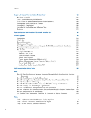
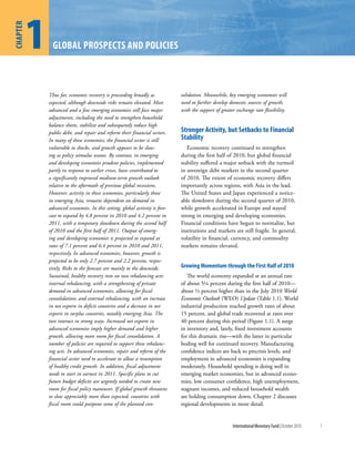
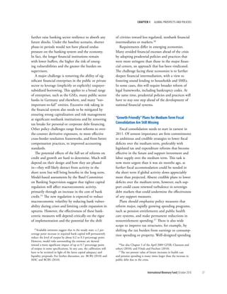
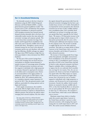
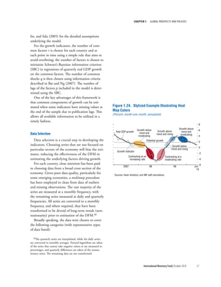
Measures included in Gregory and year” and that “much of the discrimination put in
Others (2010) place then has yet to be removed” (GTA, 2010).
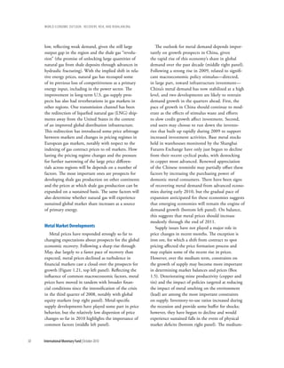
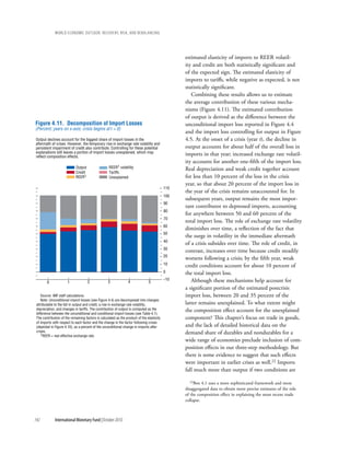
(Number of measures) Gregory and others (2010) explore the impact
Tariffs, import bans, quotas of both conventional and more unconventional
Trade defense measures “behind the border” measures highlighted in the
Nontariff barriers GTA reports, such as technical barriers to trade,
Bailouts, subsidies
procurement, and regulatory measures. The analysis
Local content, public procurement
Export measures matches data from GTA monitoring of measures
taken between mid-2008 and late 2009 with
detailed product-level data on bilateral monthly
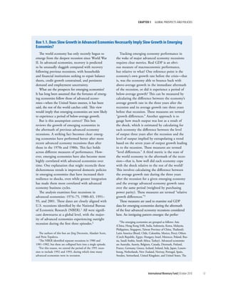
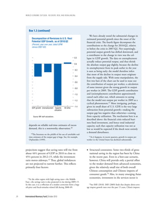
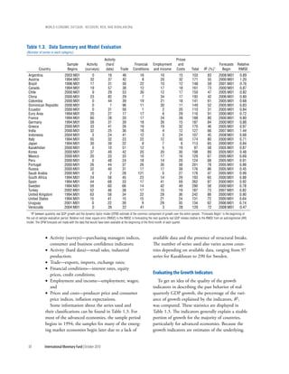
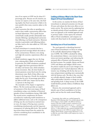
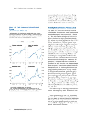
trade flows.1 The second figure illustrates the varied
51
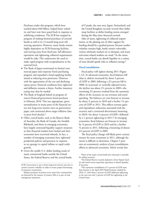
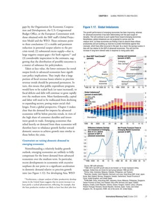
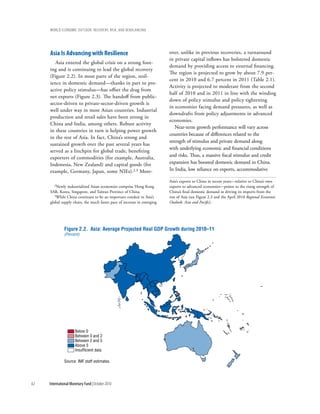
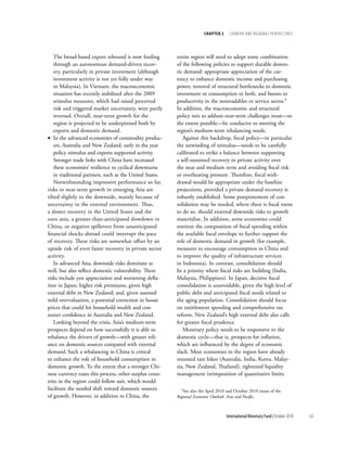
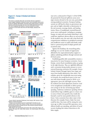
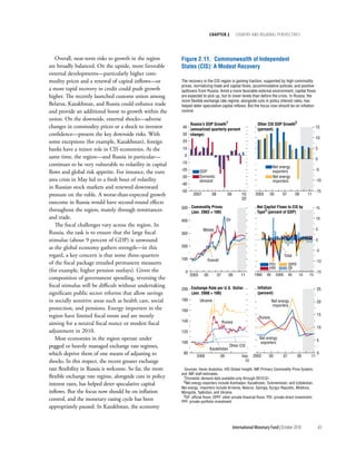
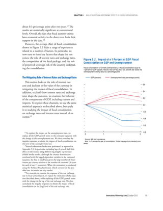
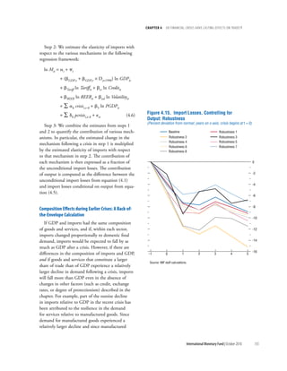
nature of these protectionist measures. There is
55 strong evidence that, after an economy imposed
import restrictions on a particular product, its
imports fell in succeeding months relative to world
trade in the same product (third figure). Allowing
for various time-varying fixed effects, more sophis-
ticated econometric analysis suggests that trade in
16
the affected products dropped an average of 3 to 8
1Extending the data set through May 2010 does not
substantially change the results of the analysis.
21 14
27
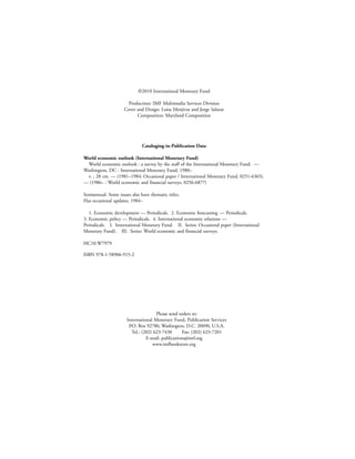
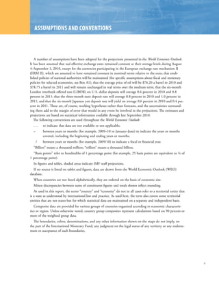
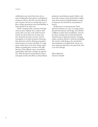
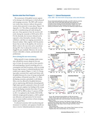
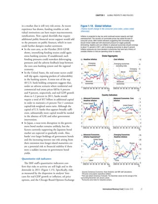
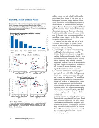
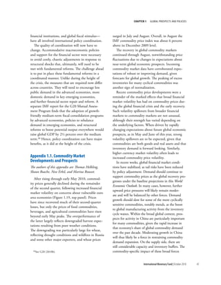
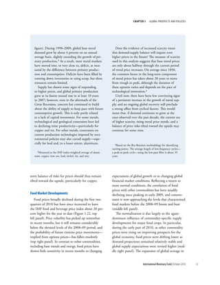
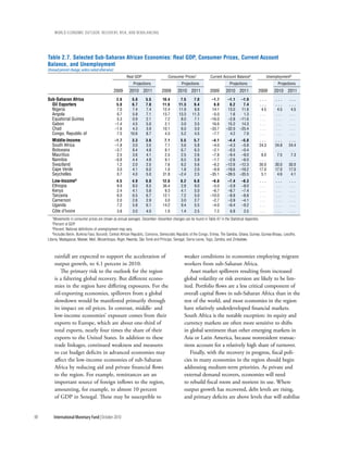
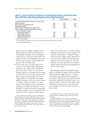
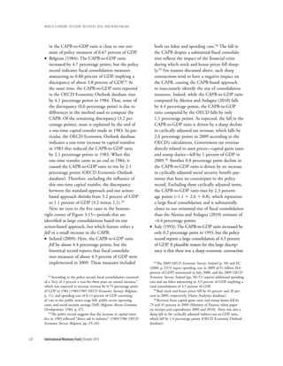
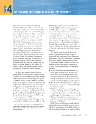
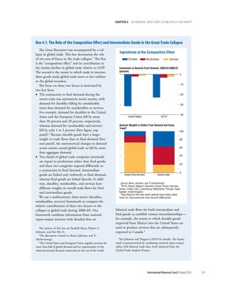
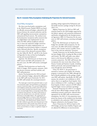
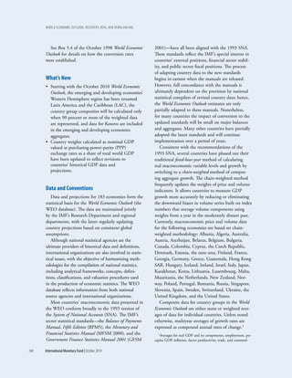
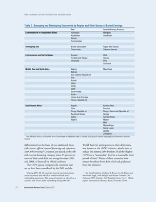
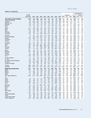
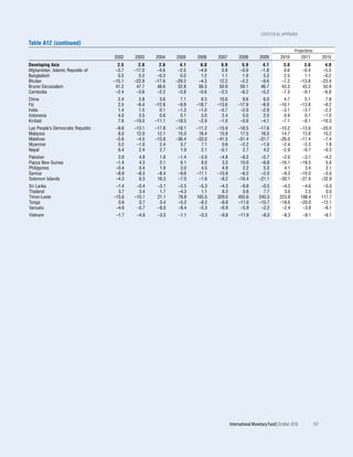
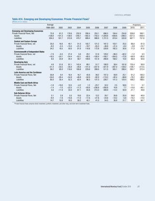
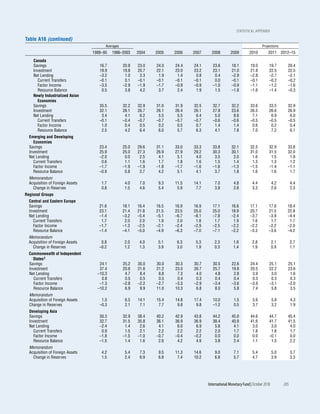
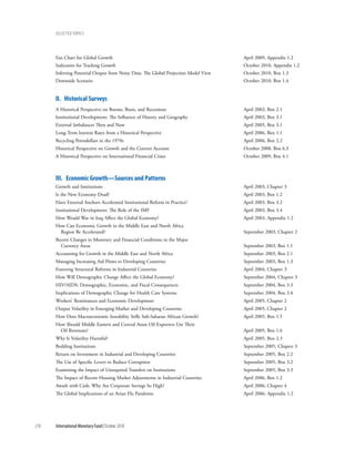
Bilateral Trade Flows subject to Measures
Implemented in November 2008
(Index, October 2008 = 100)
Source: Global Trade Alert Database.
120
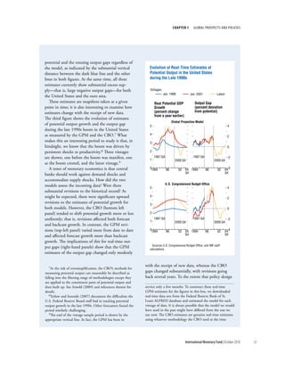
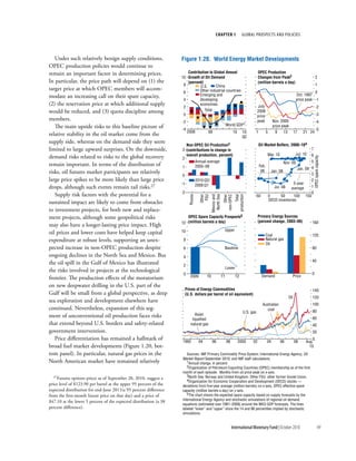
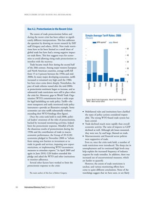
to see, an extreme protectionist surge like that of
100
the 1930s, but their assessments differ markedly.
The June 2010 joint report of the WTO, Organiza-
tion for Economic Cooperation and Development 80
(OECD), and United Nations Conference on
Trade and Development (unctad) indicates that
60
“protectionist policy responses have been limited,
although there are still instances of restrictive mea-
sures taken… [T]here continues to be few instances 40
of new import restrictions and a greater use of
export restrictions, but some G20 governments
20
have also taken steps to facilitate trade” (WTO,
OECD, and unctad, 2010). In contrast, the sixth
report of Global Trade Alert (GTA), which is asso- 0
2008 09 09 09 09
ciated with the London-based Centre for Economic
Nov. Feb. May Aug. Nov.
Policy Research and supported by the World Bank,
also released in June 2010, concludes that “as far as Source: IMF staff calculations.
open markets were concerned, 2009 was a terrible
International Monetary Fund | October 2010 147

166. wOrld ecOnOmic OutlOOk: recOvery, risk, and rebalancing
Box 4.2 (continued)
percent after the imposition of restrictions. How- Gaps in WTO commitments leave ample scope
ever, in the aggregate, restrictions implemented for further trade restrictions, and a failure by all
during the study period decreased trade by 0.25 economies to vigorously resist protectionism could
percent, because these measures affected only a threaten the economic recovery and slow future
small share of global trade. growth. Maintaining and enhancing the monitoring
Looking ahead, sustained high unemployment, of protectionist measures and sustaining high-level
uneven growth, an unwinding of government stim- political awareness of the associated macroeconomic
ulus measures, and growing economic imbalances risks will help. But the surest way to avoid such a
may increase protectionist pressure. In some econo- downside scenario is to tighten multilateral trade
mies, such pressure may also emerge from high commitments by completing the WTO Doha
commodity prices or a surge in capital inflows, Round. This can be viewed as a key part of the exit
which may lead to rapid currency appreciation. strategy from the global economic crisis.
in the absence of a financial crisis. On the other appendix 4.1. Data sources
hand, the finding that imports decline mostly for
The primary data sources for the chapter are the
investment-related goods suggests that the post-
IMF’s Direction of Trade Statistics (DOTS), World
crisis outlook for innovation and potential growth
Economic Outlook (WEO), and International
could be diminished.
Financial Statistics (IFS) databases; the NBER-UN
Domestic policymakers who might be concerned
World Trade Flows database (2005); and Laeven and
about the harmful effects of a financial crisis on
Valencia (2008, 2010). Additional data sources are
exports may be reassured by the chapter’s findings
listed in Table 4.4, and the WEO analytical regions
that declines in exports are, on average, small and
are in Table 4.5.
gradual. Moreover, these effects can be accounted
Crisis indicators are from Laeven and Valencia
for by weaker output, suggesting that addressing the
(2008, 2010). Laeven and Valencia (2010) present
factors that depress output on the supply side will new and comprehensive data on the starting dates
help exports recover as well. and characteristics of systemic banking crises over
Finally, although domestic policymakers may the period 1970–2009, building on earlier work
care more about the consequences for exports than by Caprio and others (2005), Laeven and Valencia
for imports, the global nature of the recent crisis (2008), and Reinhart and Rogoff (2009). They
means that a coordinated and protracted slump in update the Laeven and Valencia (2008) database
import demand across a wide swath of economies on systemic banking crises to include the recent
bodes ill for the global recovery. Not surprisingly, episodes following the U.S. mortgage crisis of
the chapter finds that boosting output will con- 2007 and identify 129 episodes since 1970.
siderably help imports to recover. In that regard, Laeven and Valencia (2008) also identify debt
productivity-enhancing structural reforms could crisis episodes based on sovereign debt default
help raise growth. The chapter’s findings suggest and restructuring by relying on information from
that, beyond supporting domestic demand, taking Beim and Calomiris (2001), World Bank (2002),
steps to improve credit conditions, keeping pro- Sturzenegger and Zettelmeyer (2006), and IMF
tectionist tendencies at bay, and avoiding exces- staff reports. The information compiled includes the
sive exchange rate volatility may help support the year of sovereign default on private lending and the
recovery of trade. A conclusion of the Doha Round year of debt rescheduling. Using this approach, they
of global trade talks would also reinforce the revival identify 63 episodes of sovereign debt default and
of global trade. restructuring since 1970.
148 International Monetary Fund | October 2010

167. chapter 4 dO Financial crises Have lasting eFFects On trade??
Table 4.4. Data Sources
Variable Source
Annual Data
Real Exports and Imports Direction of Trade Statistics (DOTS) Database
Real GDP in U.S. Dollars World Economic Outlook (WEO) Database
Real GDP per Capita in U.S. Dollars WEO Database
World Import/Export Price Deflator International Financial Statistics (IFS) Database
Real Effective Exchange Rate IMF
Product-Level Imports and Exports Feenstra and others (2005), COMTRADE, Pula and Peltonen (2009)
Current Account Balance WEO Database
Financial Openness Lane and Milesi-Ferretti (2007)
Trade Liberalization IMF
Bank Credit IFS Database
Production Sharing Johnson and Noguera (2010)
Debt Crisis Indicators Laeven and Valencia (2008)
Banking Crisis Indicators Laeven and Valencia (2010)
Investment Durables (machinery and equipment) Organization for Economic Cooperation and Development, Eurostat, Haver
Analytics
High-Frequency Data
Real Exports and Imports CPB Netherlands Bureau of Economic Policy Analysis, DOTS Database, Global
Trade Atlas, Haver Analytics
Antidumping Data Bown (2010)
World Import/Export Price Deflator IFS Database, CPB Netherlands Bureau of Economic Policy Analaysis
Data on bilateral and aggregate imports and Nondurables, Intermediate Goods, and Primary
exports from the DOTS database are reported in Goods, following Pula and Peltonen (2009).
current U.S. dollars. These are deflated using the The current account balance is taken from the
world import and export price deflators from the WEO database. Trade openness is measured as the
IFS database, to determine each economy’s real ratio of the sum of imports and exports to GDP.
imports and exports. The series on real GDP in Financial openness is calculated as the sum of
U.S. dollars is from the WEO database. Import- foreign assets and foreign liabilities divided by GDP,
and export-weighted partner GDP and GDP per using the updated and extended External Wealth of
capita are constructed using real GDP in U.S. dol- Nations Mark II Database (see Lane and Milesi-
lars and import and export weights from the DOTS Ferretti, 2007).
database. These weights vary each year according Bank credit to the private nonfinancial sector is
to the actual import and export flows between taken from the IFS database. Breaks in these data
economies. are identified using the IFS Country Notes publica-
Data on imports and exports by product category tion, and data are growth-spliced at these points.
are constructed from the NBER-UN World Trade The real effective exchange rate (REER) data are
Flows database (see Feenstra and others, 2005). from the IMF’s Information Notice System. The
The database is first extended using the UN volatility of the REER is calculated as the standard
COMTRADE database. The codes from the Stan- deviation of the monthly REER change in each
dard International Trade Classification, Revision 2, year. The measure of trade liberalization is from the
that identify products in the NBER-UN trade data IMF Structural Reforms Database and is described
are matched to the UN Broad Economic Classifi- in IMF (2008).
cation (BEC) codes. These are then classified into Bilateral data on production sharing are from
Capital Goods, Consumer Durables, Consumer Johnson and Noguera (2010).
International Monetary Fund | October 2010 149

168. wOrld ecOnOmic OutlOOk: recOvery, risk, and rebalancing
Table 4.5. Country Groupings
Commonwealth of
Independent States,
Advanced Economies Developing Asia Africa Georgia, Mongolia South America
Australia Afghanistan, Islamic Angola Armenia Argentina
Austria Republic of Benin Azerbaijan Bolivia
Belgium Bangladesh Botswana Belarus Brazil
Canada Bhutan Burkina Faso Georgia Chile
Cyprus Brunei Darussalam Burundi Kazakhstan Colombia
Czech Republic Cambodia Cameroon Kyrgyz Republic Ecuador
Denmark China Cape Verde Moldova Paraguay
Finland Fiji Central African Republic Mongolia Peru
France India Chad Russian Federation Uruguay
Germany Indonesia Comoros Tajikistan Venezuela
Greece Kiribati Congo, Democratic Turkmenistan Central America
Hong Kong SAR Lao People's Democratic Republic of Ukraine
Iceland Republic Congo, Republic of Uzbekistan Costa Rica
Ireland Malaysia Côte d’Ivoire El Salvador
Middle East Guatemala
Israel Maldives Djibouti
Italy Myanmar Equatorial Guinea Bahrain Honduras
Japan Nepal Eritrea Egypt Mexico
Korea Pakistan Ethiopia Iran, Islamic Republic of Nicaragua
Luxembourg Papua New Guinea Gabon Jordan Panama
Malta Philippines The Gambia Kuwait Caribbean
Netherlands Samoa Ghana Lebanon
Oman Antigua and Barbuda
New Zealand Solomon Islands Guinea
Qatar The Bahamas
Norway Sri Lanka Guinea-Bissau
Saudi Arabia Barbados
Portugal Thailand Kenya
Syrian Arab Republic Belize
Singapore Timor-Leste Lesotho
United Arab Emirates Dominica
Slovak Republic Tonga Liberia
Yemen, Republic of Dominican Republic
Slovenia Tuvalu Madagascar
Grenada
Spain Vanuatu Malawi Maghreb Guyana
Sweden Vietnam Mali
Switzerland Mauritius Algeria Haiti
Central and Eastern Libya Jamaica
Taiwan Province of China Mozambique
Europe Mauritania St. Kitts and Nevis
United Kingdom Namibia
United States Albania Niger Morocco St. Lucia
Bosnia and Herzegovina Nigeria Tunisia St. Vincent and the
Bulgaria Grenadines
Rwanda
Croatia Suriname
São Tomé and Príncipe
Estonia Trinidad and Tobago
Senegal
Hungary Seychelles
Kosovo Sierra Leone
Latvia South Africa
Lithuania Sudan
Macedonia, Former Swaziland
Yugoslav Republic of Tanzania
Montenegro Togo
Poland Uganda
Romania Zambia
Serbia Zimbabwe
Turkey
The Global Trade Atlas data at the four-digit level Japan, Korea, Russia, South Africa, Turkey, and the
of the Harmonized Commodity Description and United States. The monthly data are converted to a
Coding System (HS) are used to trace trade in types quarterly frequency, deflated by specific commod-
of products since 2001. These data cover the fol- ity price deflators—from the WEO database for
lowing: Argentina, Australia, Brazil, Canada, China, selected primary goods and from the CPB Nether-
150 International Monetary Fund | October 2010

169. chapter 4 dO Financial crises Have lasting eFFects On trade??
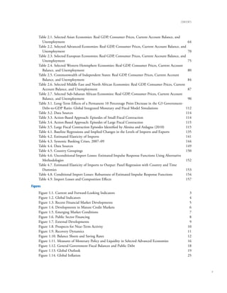
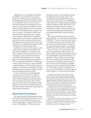
lands Bureau of Economic Policy Analysis for the following a crisis.26 In contrast to the baseline,
remaining products—and are seasonally adjusted. this methodology allows for an episode-specific
The HS four-digit codes are matched to the BEC trend, as opposed to the country-specific trend
and classified into Capital Goods, Consumer that is captured by ai in the baseline specifica-
Durables, Consumer Nondurables, Intermediate tion. However, it does not control for global
Goods, and Primary Goods, following Pula and conditions as is done in the baseline.
Peltonen (2009). • Alternative 2: Baseline specification with autore-
gressive terms—The baseline specification is
augmented by including four lags of the growth
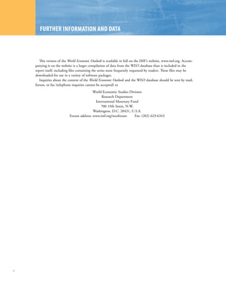
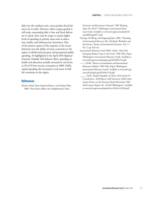
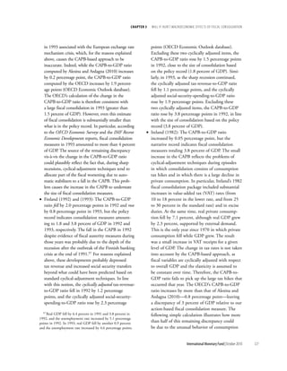
appendix 4.2. Methodology and robustness of imports on the right-hand side, paralleling the
tests specifications used in Romer and Romer (2010)
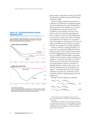
estimating Unconditional import losses and Cerra and Saxena (2008):
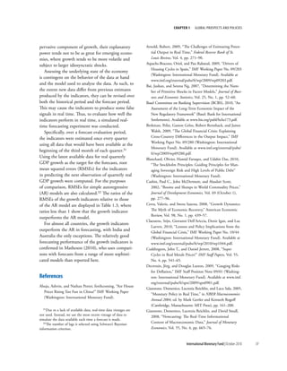
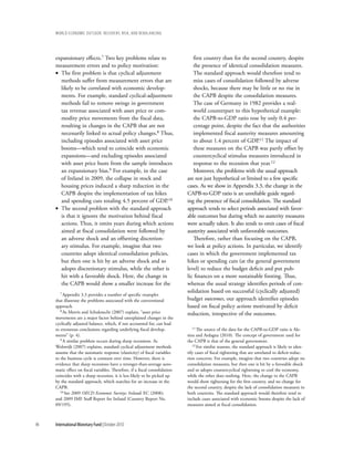
The analysis25 first estimates the unconditional D ln Mit 5 ai 1 pt 1 ∑ rl D ln Mi,t–1
dynamics of imports in the aftermath of crises using
a “collapsed” gravity model of trade in changes. 1 ∑ ak crisisi,t–k 1 eit. (4.3)
In the baseline regression specification in the text, • Alternative 3: Bilateral gravity in changes—A
the growth in an economy’s aggregate imports, directional gravity model (that is, one with bilat-
D ln Mit , is expressed as a function of a dummy eral imports or exports as opposed to bilateral
variable indicating whether a crisis started in year t, trade) is estimated in changes. The growth in
five lags of this dummy variable, and country and bilateral imports of an economy from each trad-
time dummies: ing partner, D ln Mimp,exp,t, is regressed on a crisis
D ln Mit 5 ai 1 pt 1 ∑ ak crisisi,t–k 1 eit. (4.1) indicator and its lags, as well as on time and
importer-exporter pair dummies:
The robustness of the estimated unconditional
import losses from the baseline specification is D ln Mimp,exp,t 5 aimp,exp 1 pt
verified by using the following five alternative 1 ∑ a'k crisisimp,t–k 1 eimp,exp,t . (4.4)
specifications:
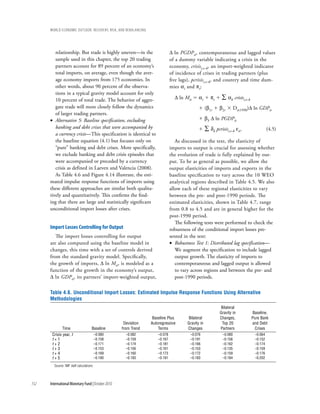
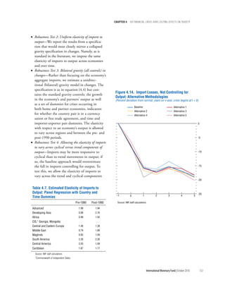
• Alternative 1: Deviation from precrisis trend— • Alternative 4: Bilateral gravity in changes, using top
This procedure measures import loss as a simple 20 partners—This specification is identical to the
deviation of ln Mit from a precrisis trend, ln Trit, directional gravity model in changes as described
where the latter is a linear trend based on a in equation (4.4) but focuses only on the top
precrisis window from (t – 7) to (t – 1). The 20 partners from which an economy imports.
mean import loss k years after a crisis is just the This is done because our primary concern is in
average of this import loss, (ln Mit – ln Trit), describing the behavior of aggregate trade, rather
across all crisis episodes. This is equivalent to than average bilateral trade. The standard gravity
estimating the following equation, either in levels model weights all bilateral trade observations
or changes: equally, regardless of the size of the bilateral trade
ln Mit 2 ln Trit 5 ∑ bk crisisi,t–k 1 eit. (4.2)
26The results from estimating equation (4.2) in levels or
This procedure is similar to the procedure changes are identical because, as in Chapter 4 of the October
2009 World Economic Outlook, the import losses are normalized
used in Chapter 4 of the October 2009 World so that the loss in the year before the crisis (t – 1) is zero. The
Economic Outlook for estimating output losses primary differences between the procedure used here and in
Chapter 4 of the October 2009 World Economic Outlook are the
following: (1) the definition of crisis (debt crises combined with
banking crises versus banking crises only), (2) the precrisis win-
25We focus on import dynamics here, since the chapter’s dow used to calculate the trend [(t – 7) to (t – 1) versus (t – 10)
results suggest that imports are where the impact of a crisis on to (t – 3)], and (3) the choice of dependent variable (imports
trade is primarily manifested. versus GDP per capita).
International Monetary Fund | October 2010 151

170. wOrld ecOnOmic OutlOOk: recOvery, risk, and rebalancing
relationship. But trade is highly uneven—in the D ln PGDPit, contemporaneous and lagged values
sample used in this chapter, the top 20 trading of a dummy variable indicating a crisis in the
partners account for 89 percent of an economy’s economy, crisisi,t–k, an import-weighted indicator
total imports, on average, even though the aver- of incidence of crises in trading partners (plus
age economy imports from 175 economies. In five lags), pcrisisi,t–k, and country and time dum-
other words, about 90 percent of the observa- mies ai and pt:
tions in a typical gravity model account for only
10 percent of total trade. The behavior of aggre- D ln Mit 5 ai 1 pt 1 ∑ ak crisisi,t–k
gate trade will more closely follow the dynamics 1 (b1r 1 b2r  Dt≥1990)D ln GDPit
of larger trading partners.
• Alternative 5: Baseline specification, excluding 1 b3 D ln PGDPit
banking and debt crises that were accompanied by 1 ∑ dk pcrisisi,t–k eit. (4.5)
a currency crisis—This specification is identical to
the baseline equation (4.1) but focuses only on As discussed in the text, the elasticity of
“pure” banking and debt crises. More specifically, imports to output is crucial for assessing whether
we exclude banking and debt crisis episodes that the evolution of trade is fully explained by out-
were accompanied or preceded by a currency put. To be as general as possible, we allow the
crisis as defined in Laeven and Valencia (2008). output elasticities of imports and exports in the
As Table 4.6 and Figure 4.14 illustrate, the esti- baseline specification to vary across the 10 WEO
mated impulse response functions of imports using analytical regions described in Table 4.5. We also
these different approaches are similar both qualita- allow each of these regional elasticities to vary
tively and quantitatively. This confirms the find- between the pre- and post-1990 periods. The
ing that there are large and statistically significant estimated elasticities, shown in Table 4.7, range
unconditional import losses after crises. from 0.8 to 4.5 and are in general higher for the
post-1990 period.
The following tests were performed to check the
import losses controlling for output robustness of the conditional import losses pre-
The import losses controlling for output sented in the text:
are also computed using the baseline model in • Robustness Test 1: Distributed lag specification—
changes, this time with a set of controls derived We augment the specification to include lagged
from the standard gravity model. Specifically, output growth. The elasticity of imports to
the growth of imports, D ln Mit, is modeled as a contemporaneous and lagged output is allowed
function of the growth in the economy’s output, to vary across regions and between the pre- and
D ln GDPit, its partners’ import-weighted output, post-1990 periods.
Table 4.6. Unconditional Import Losses: Estimated Impulse Response Functions Using Alternative
Methodologies
Bilateral
Gravity in Baseline,
Baseline Plus Bilateral Changes, Pure Bank
Deviation Autoregressive Gravity in Top 20 and Debt
Time Baseline from Trend Terms Changes Partners Crises
Crisis year, t –0.080 –0.082 –0.078 –0.076 –0.080 –0.064
t+1 –0.158 –0.159 –0.167 –0.191 –0.156 –0.152
t+2 –0.171 –0.174 –0.181 –0.166 –0.162 –0.174
t+3 –0.153 –0.156 –0.161 –0.153 –0.135 –0.159
t+4 –0.169 –0.160 –0.173 –0.172 –0.159 –0.176
t+5 –0.190 –0.183 –0.191 –0.183 –0.184 –0.202
Source: IMF staff calculations.
152 International Monetary Fund | October 2010

171. chapter 4 dO Financial crises Have lasting eFFects On trade??
• Robustness Test 2: Uniform elasticity of imports to
output—We report the results from a specifica-
tion that would most closely mirror a collapsed
gravity specification in changes. Namely, as is
standard in the literature, we impose the same
elasticity of imports to output across economies
and over time.
• Robustness Test 3: Bilateral gravity (all controls) in
changes—Rather than focusing on the economy’s
aggregate imports, we estimate a unidirec-
tional (bilateral) gravity model in changes. The
specification is as in equation (4.4) but con-
Figure 4.14. Import Losses, Not Controlling for
tains the standard gravity controls: the growth
Output: Alternative Methodologies
in the economy’s and partners’ output as well (Percent deviation from normal; years on x-axis; crisis begins at t = 0)
as a set of dummies for crises occurring in
Baseline Alternative 1
both home and partner economies, indicators
Alternative 2 Alternative 3
for whether the country pair is in a currency Alternative 4 Alternative 5
union or free trade agreement, and time and
importer-exporter pair dummies. The elasticity 0
with respect to an economy’s output is allowed
to vary across regions and between the pre- and
post-1990 periods. -5
• Robustness Test 4: Allowing the elasticity of imports
to vary across cyclical versus trend components of
output—Imports may be more responsive to -10
cyclical than to trend movements in output; if
so, the baseline approach would overestimate
the fall in imports controlling for output. To -15
test this, we allow the elasticity of imports to
vary across the trend and cyclical components
-20
Table 4.7. Estimated Elasticity of Imports to
Output: Panel Regression with Country and -25
–1 0 1 2 3 4 5
Time Dummies
Pre-1990 Post-1990 Source: IMF staff calculations.
Advanced 1.99 1.94
Developing Asia 0.89 2.76
Africa 0.99 1.50
CIS,1 Georgia, Mongolia ... ...
Central and Eastern Europe 1.46 1.38
Middle East 0.79 1.89
Maghreb 0.83 1.09
South America 2.26 2.26
Central America 2.03 1.58
Caribbean 1.87 1.77
Source: IMF staff calculations.
1Commonwealth of Independent States.
International Monetary Fund | October 2010 153

172. wOrld ecOnOmic OutlOOk: recOvery, risk, and rebalancing
of output, where the trend and cycle were ods—Similar to Robustness Test 4, the sensitivity
separated using a Hodrick-Prescott filter. As in of imports to output may be particularly high
the baseline, the import elasticity with respect in times of crisis. We thus allow the coefficient
to both the cyclical and trend components of on output to vary during crisis and noncrisis
output are allowed to vary across WEO regions periods.
and between the pre- and post-1990 periods. The results of these robustness tests are presented
• Robustness Test 5: Controlling for changes in the in Table 4.8 and Figure 4.15. The finding that
REER and relative prices—Import dynamics may imports remain below their normal levels following
differ after crises due to changes in the REER a crisis, even after controlling for output, is con-
and relative price levels. Equation (4.5) is aug- firmed across all these robustness checks. While the
mented to control for changes in REER and the standard errors increase substantially once we allow
domestic price level, proxied by the change in the the estimated elasticity of imports to output to vary
GDP deflator. across economies, the point estimates remain very
• Robustness Test 6: Controlling for changes in similar to the baseline specification.
domestic aggregate demand—An economy’s GDP
may not be a good proxy for absorption in
the importing economy, and to the extent that Decomposition of Unconditional import losses
absorption declines more than GDP during cri- We use a three-step approach to evaluate the
ses, the estimated import losses after controlling importance of different mechanisms in explaining
for output may be overstated. We replace growth the unconditional import losses, as detailed below.
in output by growth in domestic absorption It is important to keep in mind that this is simply
(consumption plus investment) on the right-hand an accounting exercise that attempts to decompose
side of equation (4.5). the unconditional import losses based on observed
• Robustness Test 7: Allowing the elasticity of imports correlations. The true contributions of the vari-
to output to differ across economies—We further ous mechanisms might differ from these estimated
increase the flexibility of our specification by correlations.
estimating separately the elasticity of imports Step 1: We document whether crises are followed
to output for each of the 154 economies in the by persistent changes in tariffs, credit, the REER,
sample. and exchange rate volatility by estimating equation
• Robustness Test 8: Allowing the elasticity of imports (4.1) with the mechanisms of interest as the depen-
to output to vary across crisis versus noncrisis peri- dent variable.
Table 4.8. Conditional Import Losses: Robustness of Estimated Impulse Response Functions
Baseline Same Control for
and Elasticity Control for Changes in Elasticity:
Lagged across Elasticity: Changes in Consumption Elasticity: Differs
Growth of Regions Full Gravity Cyclical vs. REER and and Varies by during
Time Baseline Output and Time in Changes Trend PPP1 Investment Economy Crisis Years
(1) (2) (3) (4) (5) (6) (7) (8) (9)
Crisis year, t –0.040*** –0.037** –0.058*** –0.022* –0.043*** –0.052*** –0.042*** –0.031* –0.052***
t+1 –0.073*** –0.074*** –0.116*** –0.093*** –0.076*** –0.090*** –0.079*** –0.058** –0.114***
t+2 –0.077*** –0.086*** –0.129*** –0.053*** –0.086*** –0.092*** –0.093*** –0.054* –0.122***
t+3 –0.063* –0.071** –0.114*** –0.048** –0.077** –0.074*** –0.076*** –0.041 –0.099***
t+4 –0.077** –0.081*** –0.133*** –0.074*** –0.090*** –0.091*** –0.087*** –0.057* –0.101***
t+5 –0.089** –0.092*** –0.152*** –0.068*** –0.099*** –0.105*** –0.095*** –0.071* –0.115***
Source: IMF staff calculations.
Note: All columns include economy- and year-fixed effects. Columns (1), (2), and (4) – (7) allow the elasticity of imports to output (or its cyclical and trend component and consump-
tion and investment) to vary by WEO regions and after 1990. In column (8), the elasticity of imports to output is allowed to vary by economy.
1REER = real effective exchange rate; PPP = purchasing power parity.
154 International Monetary Fund | October 2010

173. chapter 4 dO Financial crises Have lasting eFFects On trade??
Step 2: We estimate the elasticity of imports with
respect to the various mechanisms in the following
regression framework:
ln Mit = ai + pt
+ (bGDP,r + bGDP,r × Dt≥1990) ln GDPit
+ bTariff ln Tariffit + bcr ln Creditit
+ bREER ln REERit + bvol ln Volatilityit
+ ∑ ak crisisi,t–k + b3 ln PGDPit
+ ∑ dk pcrisisi,t–k + it (4.6) Figure 4.15. Import Losses, Controlling for
Output: Robustness
(Percent deviation from normal; years on x-axis; crisis begins at t = 0)
Step 3: We combine the estimates from steps 1
and 2 to quantify the contribution of various mech- Baseline Robustness 1
anisms. In particular, the estimated change in the Robustness 2 Robustness 3
Robustness 4 Robustness 5
mechanism following a crisis in step 1 is multiplied
Robustness 6 Robustness 7
by the estimated elasticity of imports with respect Robustness 8
to that mechanism in step 2. The contribution of
each mechanism is then expressed as a fraction of 0
the unconditional import losses. The contribution
of output is computed as the difference between the -2
unconditional import losses from equation (4.1)
-4
and import losses conditional on output from equa-
tion (4.5).
-6
-8
composition effects during earlier crises: a Back-of-
the-envelope calculation
-10
If GDP and imports had the same composition
of goods and services, and if, within each sector, -12
imports changed proportionally to domestic final
demand, imports would be expected to fall by as -14
much as GDP after a crisis. However, if there are
-16
differences in the composition of imports and GDP, –1 0 1 2 3 4 5
and if goods and services that constitute a larger
Source: IMF staff calculations.
share of trade than of GDP experience a relatively
larger decline in demand following a crisis, imports
will fall more than GDP even in the absence of
changes in other factors (such as credit, exchange
rates, or degree of protectionism) described in the
chapter. For example, part of the outsize decline
in imports relative to GDP in the recent crisis has
been attributed to the resilience in the demand
for services relative to manufactured goods. Since
demand for manufactured goods experienced a
relatively larger decline and since manufactured
International Monetary Fund | October 2010 155

174. wOrld ecOnOmic OutlOOk: recOvery, risk, and rebalancing
goods comprise a larger share of trade than of GDP,
overall imports declined more than GDP (Borchert
and Mattoo, 2009).
We first investigate whether historically there is
a difference in the behavior of manufactured goods
and services following crises. Since detailed data on
the demand side are not available, we use sectoral
value-added data to document whether there
are differences in the behavior of services versus
Figure 4.16. The Postcrisis Evolution of Various
industry after crises. Somewhat surprisingly, this
Components of GDP
(Percent deviation from normal; years on x-axis; crisis begins at t = 0) does not appear to be the case. The estimated drop
in services is very similar to the decline in industry
Crises are followed by roughly equal declines in services and industry. The
postcrisis decline in investment in machinery and equipment, on the other value added after crises (Figure 4.16, top panel).27
hand, is much deeper than for the rest of output. Given this similarity in the dynamics of services and
industry, the different shares of services in output
Services, Industry, and Total Output
0 and trade do not appear to be a likely explanation.
However, within the “manufactured goods” cat-
-2
egory, there are compositional differences between
Total output -4 output and trade. Across a sample of 48 economies
for which disaggregated data on gross fixed invest-
Services -6 ment are available, (capital) durables, measured by
tradable investment goods—namely, machinery and
Industry -8
equipment—account for only 8 percent of GDP.
-10 For the same set of economies, the average share
–1 0 1 2 3 4 5
of (capital) durables in imports is 18 percent.28
Durables and the Rest of Output
Although the data coverage is rather scant—only
0
26 of the identified crises can be included in the
Rest of output analysis— we provide some back-of-the-envelope
-10 calculations to estimate the contribution of these
composition effects in explaining import losses fol-
-20 lowing crises.
Durables
We begin with the following two identities:
-30
GDPgth = shdur × DURGDP
GDP gth
–1 0 1 2 3 4 5
-40 + (1 – shdur ) × OTHERGDP (4.7)
GDP gth
IMPgth = shdur × DURIMP
Source: IMF staff calculations. IMP gth
Note: Lines indicate the impulse response function – the effect of a crisis on imports
relative to what would be predicted in the absence of a crisis. Predictions are based on + (1 – shdur ) × OTHERIMP , (4.8)
IMP gth
contemporaneous and lagged crises, and country and time dummies.
27The overall output loss is slightly lower than the loss of
services and industry due to the resilience of agricultural produc-
tion to crises.
28The definition of “durables” in the trade and output data is
not identical because these series come from different, not always
comparable, data sources. However, it is unlikely that differences
in definitions account for the differences in the shares of these
goods in imports and output.
156 International Monetary Fund | October 2010

175. chapter 4 dO Financial crises Have lasting eFFects On trade??
where GDPgth and IMPgth are the growth rates in Table 4.9 and Figure 4.16 present the findings
GDP and imports, respectively; shdur and shdur from this exercise. The impulse response functions
GDP IMP
are the share of (capital) durables in GDP and of investment in machinery and equipment and
imports, respectively; DURGDPgth and DURIMPgth are the rest of GDP are shown in Figure 4.16 (bottom
the growth rate in the (capital) durable component panel).29 The postcrisis decline in investment, and
of GDP and imports, respectively; and OTHERGDPgth in particular in machinery and equipment, is much
and OTHERIMPgth are the growth rate in other com- larger than the postcrisis decline in the rest of GDP
ponents of GDP and imports, respectively. over the same period. As presented in column (6)
Assuming the elasticity of imports of different prod- of Table 4.9, for this selected sample of crises, the
ucts to GDP is 1, equation (4.8) can be rewritten as composition effect can explain 5 to 13 percent of
the unconditional import loss. It is important to
IMPgth = shdur × DURGDP
IMP gth keep in mind that these composition effects are
+ (1 – shdur ) × OTHERGDP . (4.9) calculated only from the different shares and post-
IMP gth
crisis behavior of machinery and equipment relative
Subtracting (4.7) from (4.9) implies
to the rest of output; other composition effects—
IMPgth – GDPgth = (shdur – shdur ) most notably, from consumer durables—may
IMP GDP
also be present. In addition, composition effects
× (DURGDP – OTHERGDP ). (4.10)
gth gth may already be reflected in the higher elasticity of
Based on equation (4.10), we define the compo- imports to output that is allowed for in our baseline
sition effect as the extent to which the difference specification. Thus, these estimates of the size of the
between the growth rates of GDP and imports is composition effect could be thought of as a lower
explained by different compositions of GDP and bound.
imports. It is a product of two factors: (1) differ-
ences in the share of durables in imports and GDP
and (2) differences in the growth of durables and
other components following a crisis. If either of
these differences is zero, composition cannot be an 29Given the share of durables in GDP, as well as the decline in
explanation for observing import losses controlling overall GDP, we can also calculate how much demand for other
for output. components of GDP falls after crises.
Table 4.9. Import Losses and Composition Effects
Implied Response Function
Actual Estimated Share of Import
Investment Import Composition Loss Explained by
GDP in Durables Other Loss Effect Composition Effects
Time (1) (2) (3) (4) (5) (6)
Crisis year, t –0.024 –0.091 –0.018 –0.088 –0.007 8.0
t+1 –0.051 –0.285 –0.029 –0.267 –0.025 9.2
t+2 –0.054 –0.340 –0.028 –0.250 –0.030 12.1
t+3 –0.050 –0.234 –0.033 –0.155 –0.019 12.6
t+4 –0.048 –0.160 –0.038 –0.153 –0.012 7.7
t+5 –0.049 –0.114 –0.043 –0.144 –0.007 4.8
Source: IMF staff calculations.
Note: All estimates in columns (1), (2), and (4) are significant at the 1 percent level. Standard errors (not reported) are clustered by economy and corrected for heterosce-
dasticity. The actual import loss is estimated for the subsample of economies and crises for which disaggregated investment data are available. The share of import loss
explained by composition effects in column (6) is calculated as the estimated composition effect in column (5) divided by the actual import loss multiplied by 100.
International Monetary Fund | October 2010 157

176. wOrld ecOnOmic OutlOOk: recOvery, risk, and rebalancing
references Bown, Chad, 2010, “Fourth Quarter 2009 Protectionism
Data: Requests for New Trade Barriers Fall for the First
Abiad, Abdul, Giovanni Dell’Ariccia, and Bin Li, forthcom- Time in Crisis; But Newly Imposed Barriers Increase,” a
ing, “Creditless Recoveries,” IMF Working Paper (Wash- Monitoring Update to the Global Antidumping Database,
ington: International Monetary Fund). February (Washington: World Bank).
Alessandria, George, Joseph P. Kaboski, and Virgiliu Caprio, Gerard, Daniela Klingebiel, Luc Laeven, and
Midrigan, forthcoming, “The Great Trade Collapse of Guillermo Noguera, 2005, “Appendix: Banking Crisis
2008–09: An Inventory Adjustment?” IMF Economic Database,” in Systemic Financial Crises: Containment
Review, (Washington: International Monetary Fund). and Resolution, ed. by Patrick Honohan and Luc Laeven
Altomonte, Carlo, and Gianmarco I.P. Ottaviano, 2009, (Cambridge, United Kingdom: Cambridge University
“Resilient to the Crisis? Global Supply Chains and Trade Press).
Flows,” in The Great Trade Collapse: Causes, Consequences Cerra, Valerie, and Sweta Saxena, 2008, “Growth Dynamics:
and Prospects, ed. by Richard Baldwin. Available at www. The Myth of Economic Recovery,” American Economic
voxeu.org/index.php?q=node/4289. Review, Vol. 98, No. 1, pp. 439–57.
Amiti, Mary, and David E. Weinstein, 2009, “Exports and Chor, Davin, and Kalina Manova, 2010, “Off the Cliff and
Financial Shocks,” NBER Working Paper No. 15556 Back? Credit Conditions and International Trade during
(Cambridge, Massachusetts: National Bureau of Economic the Global Financial Crisis” (unpublished; Stanford, Cali-
Research). fornia: Stanford University).
Anderson, James, and Eric Van Wincoop, 2003, “Gravity Eaton, Jonathan, Sam Kortum, Brent Neiman, and John
with Gravitas: A Solution to the Border Puzzle,” American Romalis, 2010, “Trade and the Global Recession” (unpub-
Economic Review, Vol. 93, No. 1, pp. 170–92. lished; Chicago, Illinois: University of Chicago). Available
Baldwin, Richard, 1988, “Hysteresis in Import Prices: The at http://home.uchicago.edu/~kortum/papers/EKNR.pdf.
Beachhead Effect,” American Economic Review, Vol. 78, Feenstra, Robert, Robert Lipsey, Haiyan Deng, Alyson Ma,
No. 4, pp. 773–85. and Hengyong Mo, 2005, “World Trade Flows: 1962–
———, ed., 2009, The Great Trade Collapse: Causes, Conse- 2000,” NBER Working Paper No. 11040 (Cambridge,
quences and Prospects. Available at www.voxeu.org/index. Massachusetts: National Bureau of Economic Research).
php?q=node/4297. Frankel, Jeffrey, Ernesto Stein, and Shang-Jin Wei, 1996,
———, and Daria Taglioni, 2006, “Gravity for Dummies “Regional Trading Arrangements: Natural or Supernatural?”
and Dummies for Gravity Equations,” NBER Working American Economic Review, Vol. 86, No. 2, pp. 52–56.
Paper No. 12516 (Cambridge, Massachusetts: National Friedman, Jed, and James Levinsohn, 2003, “The Distribu-
Bureau of Economic Research). tional Impacts of Indonesia’s Financial Crisis on Household
Beim, David, and Charles Calomiris, 2001, Emerging Welfare: A ‘Rapid Response’ Methodology,” The World
Financial Markets, appendix to Chapter 1 (New York: Bank Economic Review, Vol. 16, No. 3, pp. 397–423.
McGraw-Hill/Irwin). Freund, Caroline, 2009, “The Trade Response to Global
Bems, Rudolfs, Robert Johnson, and Kei-Mu Yi, forthcom- Downturns: Historical Evidence,” Policy Research Work-
ing, “Demand Spillovers and the Collapse of Trade in the ing Paper No. 5015 (Washington: World Bank).
Global Recession,” IMF Economic Review (Washington: Glick, Reuven, and Alan M. Taylor, 2010, “Collateral Dam-
International Monetary Fund). age: Trade Disruption and the Economic Impact of War,”
Berman, Nicolas, and Philippe Martin, 2010, “The The Review of Economics and Statistics, Vol. 92, No. 1, pp.
Vulnerability of Sub-Saharan Africa to the Financial 102–27.
Crisis: The Case of Trade,” CEPR Discussion Paper Global Trade Alert, 2010, “Unequal Compliance: The 6th
No. 7765 (London: Centre for Economic Policy GTA Report” (London). Available at www.globaltrade
Research). alert.org/gta-analysis/unequal-compliance-6th-gta-report.
Bernard, Andrew, J. Bradford Jensen, Stephen J. Redding, Gregory, Rob, Christian Henn, Brad McDonald and Mika
and Peter K. Schott, 2009, “The Margins of U.S. Trade,” Saito, 2010, “Trade and the Crisis: Protect or Recover,”
American Economic Review Papers and Proceedings, Vol. 99, IMF Staff Position Note 10/07 (Washington: Interna-
No. 2, pp. 487–93. tional Monetary Fund).
Borchert, Ingo, and Aaditya Mattoo, 2009, “The Crisis-Resil- Iacovone, Leonardo, and Veronika Zavacka, 2009, “Banking
ience of Services Trade,” Policy Research Working Paper Crises and Exports: Lessons from the Past,” Policy Research
4917 (Washington: World Bank). Working Paper No. 5016 (Washington: World Bank).
158 International Monetary Fund | October 2010

177. chapter 4 dO Financial crises Have lasting eFFects On trade??
International Monetary Fund (IMF), 2008, “Structural Pula, Gabor, and Tuomas Peltonen, 2009, “Has Emerging
Reforms and Economic Performance in Advanced and Asia Decoupled? An Analysis of Production and Trade
Developing Countries,” Research Department paper. Avail- Linkages Using the Asian International Input-Output
able at www.imf.org/external/np/res/docs/2008/0608.htm. Table,” ECB Working Paper No. 993 (Frankfurt: Euro-
Johnson, Robert C., and Guillermo Noguera, 2010, pean Central Bank).
“Accounting for Intermediates: Production Sharing and Reinhart, Carmen, and Kenneth Rogoff, 2009, This Time
Trade in Value Added” (unpublished; Hanover, New Is Different: Eight Centuries of Financial Folly (Princeton,
Hampshire: Dartmouth College). New Jersey: Princeton University Press).
Kaminsky, Graciela, L., and Carmen M. Reinhart, 1999, Romer, Christina, and David Romer, 2010, “The Macroeco-
“The Twin Crises: The Causes of Banking and Balance of nomic Effects of Tax Changes: Estimates Based on a New
Payments Problems,” American Economic Review, Vol. 89, Measure of Fiscal Shocks,” American Economic Review,
No. 3, pp. 473–500. Vol. 100, No. 3, pp. 763–801.
Kwack, Sung Yeung, Choong Y. Ahn, Young S. Lee, and Ronci, Marcio, 2004, “Trade Finance and Trade Flows: Panel
Doo Y. Yang, 2007, “Consistent Estimates of World Trade Data Evidence from 10 Crises,” IMF Working Paper
Elasticities and an Application to the Effects of Chinese 04/225 (Washington: International Monetary Fund).
Yuan (RMB) Appreciation,” Journal of Asian Economics, Rose, Andrew, 2000, “One Money, One Market: Estimating
Vol. 18, No. 2, pp. 314–30. the Effect of Common Currencies on Trade,” Economic
Laeven, Luc, and Fabian Valencia, 2008, “Systemic Banking Policy, Vol. 15, No. 30, pp. 7–46.
Crises: A New Database,” IMF Working Paper 08/224 Senhadji, Abdelhak, 1998, “Time-Series Estimation of
(Washington: International Monetary Fund). Structural Import Demand Equations: A Cross-country
———, 2010, “Resolution of Banking Crises: The Good, Analysis,” IMF Staff Papers, Vol. 45, No. 2 (Washington:
the Bad, and the Ugly,” IMF Working Paper 10/146 International Monetary Fund).
(Washington: International Monetary Fund). Sturzenegger, Federico, and Jeromin Zettelmeyer, 2006, Debt
Lane, Philip R., and Gian Maria Milesi-Ferretti, 2007, “The Defaults and Lessons from a Decade of Crises, Chapter 1,
External Wealth of Nations Mark II,” Journal of Interna- Table 1 (Cambridge, Massachusetts: MIT Press).
tional Economics, Vol. 73, No. 2, pp. 223–50. Thursby, Marie, and Jerry Thursby, 1987, “Bilateral Trade
Levchenko, Andrei, Logan Lewis, and Linda Tesar, forth- Flows, the Linder Hypothesis, and Exchange Risk,”
coming, “The Collapse of International Trade during the Review of Economics and Statistics, Vol. 69, No. 3, pp.
2008-2009 Crisis: In Search of the Smoking Gun,” IMF 488–95.
Economic Review (Washington: International Monetary World Bank, 2002, Global Development Finance, appendix
Fund). on commercial debt restructuring (Washington: World
Martin, Philippe, Thierry Mayer, and Mathias Thoenig, Bank).
2008, “Make Trade, Not War?” Review of Economic Stud- World Trade Organization (WTO), Organization for
ies, Vol. 75, No. 3, pp. 865–900. Economic Cooperation and Development (OECD), and
O’Rourke, Kevin, 2009, “Government Policies and the Col- United Nations Conference on Trade and Development
lapse in Trade during the Great Depression,” in The Great (UNCTAD), 2010, “Report on G20 Trade and Invest-
Trade Collapse: Causes, Consequences and Prospects, ed. ment Measures (November 2009 to Mid-May 2010)”
by Richard Baldwin. Available at www.voxeu.org/index. (Paris, June). Available at www.unctad.org/templates/
php?q=node/4267. Download.asp?docid=13369&lang=1.
International Monetary Fund | October 2010 159

179. Annex
IMF executIve BoArd dIscussIon oF the outlook, septeMBer 2010
The following remarks by the Acting Chair were made at the conclusion of the Executive Board’s discussion of the
World Economic Outlook on September 20, 2010.
E
xecutive Directors observed that the global and debt stabilization, including through legislation
economic recovery is proceeding broadly as where necessary. At the same time, policymakers
projected, despite disturbances in financial should stand ready to act if global growth threatens
markets. The recovery is losing momen- to slow appreciably more than expected. In this
tum temporarily during the second half of 2010 and regard, consideration could be given to postpon-
will likely remain weak in the first half of 2011, as ing consolidation in countries with fiscal room and
extraordinary policy stimulus is gradually withdrawn. credibility to do so. In all but the most vulnerable
Directors welcomed signs that financial conditions countries, automatic stabilizers should be allowed to
have begun to normalize, aided by policy coordina- operate. Directors stressed that medium-term con-
tion and announcements of a front-loading of fiscal solidation plans should be based on realistic growth
adjustment in Europe. A more robust, self-sustaining projections and include reforms to limit rapidly
global recovery will require progress in achieving escalating spending programs such as pension enti-
both internal and global demand rebalancing, sup- tlements and public health care and tax incentives
ported by healthy financial systems. to boost the supply potential and discourage debt.
Directors noted that the observed asymmetry In light of subdued inflation pressures, Direc-
in growth performances will likely persist. In most tors generally considered that monetary policy in
advanced and a few emerging market economies, most advanced economies should remain highly
recoveries are proceeding at a sluggish pace, and accommodative, including through unconventional
large internal adjustments remain needed to achieve measures if needed, and should be the first line of
internal rebalancing from stimulus-led to private- defense against any larger-than-projected weakening
sector-led growth. On the other hand, growth in of activity as fiscal stimulus is being unwound. In
many emerging market and developing economies emerging market economies with rising inflation or
continues to be vigorous, on the back of improved asset price pressures, monetary tightening has been
macroeconomic policy frameworks and a stronger broadly appropriate. For all economies, the impli-
financial footing. Downside risks to near-term cations of fiscal consolidation and developments
global growth remain elevated and concentrated in in financial and asset markets for inflation would
advanced economies. These emanate from height- also need to be taken into account when setting
ened uncertainty in financial markets, fragile real monetary policy.
estate markets, continued household deleveraging, Directors underscored the urgent need for restor-
and persistently high unemployment. However, the ing financial sector health and making progress
probability of a sharp global slowdown, including in regulatory reforms in a coordinated manner,
stagnation or contraction in advanced economies, especially among advanced economies. To enable
appears low. an early exit from fiscal support as well as address
Directors agreed that fiscal consolidation is a legacy problems, priorities include restructuring and
top priority in countries with relatively high public resolving weak financial institutions; implementing
debt. They highlighted the urgency of adopting measures to shore up bank capital adequacy, liquid-
credible strategies for medium-term consolidation ity, and stability of funding sources; and improving
International Monetary Fund | October 2010 161

180. wOrld ecOnOmic OutlOOk: recOvery, risk, and rebalancing
coordination of supervision to avoid rapid cross- account deficits. Continued fiscal adjustment and
border amplification of shocks. Further advance- financial sector reforms that discourage excessive
ment toward building a stronger financial regulatory spending are also key.
framework is crucial to underpin market confidence Directors noted that structural policies that
and enhance global financial stability. strengthen growth over the medium term would
Directors emphasized that medium-term growth help support the required normalization of macro-
prospects depend on progress in implementing economic policies in advanced economies. Labor
structural policies to give forceful impetus to global market policies, coupled with complementary
demand rebalancing. In this regard, many emerging product and services market reforms, should aim
market economies would need to further reorient to promote competition and enhance growth and
toward domestic demand, not only because import job creation, and with sufficient support for the
recovery in advanced economies will likely trail unemployed.
behind precrisis trends, but also to achieve balanced Directors underscored the critical importance of
growth that addresses their own consumption and continued policy effort and coordination at both
investment needs. For economies with excessive the regional and global levels—as demonstrated
external surpluses, this would entail allowing further during the global crisis and more recently during
exchange rate flexibility and appreciation in response the European sovereign debt market turmoil. While
to sustained capital inflows, while safeguarding finan- policy requirements now differ considerably across
cial stability with macroprudential or other targeted countries, it is essential that countries continue to
measures. These measures should be complemented work together toward the common goal of achiev-
by structural reforms aimed at enhancing social safety ing strong, sustained, and balanced growth over
nets and shifting toward optimal saving-investment the medium term. Directors also emphasized the
patterns. Similarly, measures to boost net exports need to avoid negative spillovers as well as trade and
would be crucial for economies with excessive current investment protectionism.
162 International Monetary Fund | October 2010

181. StatiStical appendix
T
he Statistical Appendix presents his- assumptions underlying the projections for selected
torical data, as well as projections. It economies are described in Box A1.
comprises five sections: Assumptions, With regard to interest rates, it is assumed that
What’s New, Data and Conventions, the London interbank offered rate (LIBOR) on six-
Classification of Countries, and Statistical Tables. month U.S. dollar deposits will average 0.6 percent
The assumptions underlying the estimates and in 2010 and 0.8 percent in 2011, that three-month
projections for 2010–11 and the medium-term sce- euro deposits will average 0.8 percent in 2010 and
nario for 2012–15 are summarized in the first sec- 1.0 percent in 2011, and that six-month yen depos-
tion. The second section presents a brief description its will average 0.6 percent in 2010 and 0.4 percent
of changes to the database and statistical tables. in 2011.
The third section provides a general description of With respect to introduction of the euro, on
the data and of the conventions used for calculat- December 31, 1998, the Council of the European
ing country group composites. The classification Union decided that, effective January 1, 1999, the
of countries in the various groups presented in irrevocably fixed conversion rates between the euro
the World Economic Outlook is summarized in the and currencies of the member states adopting the
fourth section. euro are as follows.
The last, and main, section comprises the statis-
tical tables. Data in these tables have been com-
piled on the basis of information available through 1 euro = 13.7603 Austrian schillings
late September 2010. The figures for 2010 and = 40.3399 Belgian francs
beyond are shown with the same degree of preci- = 0.585274 Cyprus pound1
sion as the historical figures solely for convenience; = 1.95583 Deutsche mark
because they are projections, the same degree of = 5.94573 Finnish markkaa
accuracy is not to be inferred. = 6.55957 French francs
= 340.750 Greek drachma2
assumptions = 0.787564 Irish pound
= 1,936.27 Italian lire
Real effective exchange rates for the advanced
= 40.3399 Luxembourg francs
economies are assumed to remain constant at their
= 0.42930 Maltese lira3
average levels during the period August 4–Septem-
= 2.20371 Netherlands guilders
ber 1, 2010. For 2010 and 2011, these assumptions
= 200.482 Portuguese escudos
imply average U.S. dollar/SDR conversion rates of
= 30.1260 Slovak koruna4
1.516 and 1.520, U.S. dollar/euro conversion rates
= 239.640 Slovenian tolars5
of 1.308 and 1.284, and yen/U.S. dollar conversion
= 166.386 Spanish pesetas
rates of 88.5 and 84.2, respectively.
It is assumed that the price of oil will average
1Established on January 1, 2008.
$76.20 a barrel in 2010 and $78.75 a barrel in
2Established on January 1, 2001.
2011. 3Established on January 1, 2008.
Established policies of national authorities are 4Established on January 1, 2009.
assumed to be maintained. The more specific policy 5Established on January 1, 2007.
International Monetary Fund | October 2010 163

182. WOrld EcOnOmic OutlOOk: rEcOvEry, risk, and rEbalancing
Box a1. economic policy assumptions Underlying the projections for Selected economies
Fiscal Policy Assumptions spending ceilings (approved by Parliament) and
The short-term fiscal policy assumptions used the health insurance package savings for all years
in the World Economic Outlook (WEO) are based (2011–15).
on officially announced budgets, adjusted for dif- Belgium: Projections for 2010 are IMF staff
ferences between the national authorities and the estimates based on the 2010 budgets approved by
IMF staff regarding macroeconomic assumptions the federal, regional, and community parliaments
and projected fiscal outturns. The medium-term and further strengthened by the Intergovernmen-
fiscal projections incorporate policy measures that tal Agreement 2009–10. Projections for the outer
are judged likely to be implemented. In cases years are IMF staff estimates, assuming unchanged
where the IMF staff has insufficient informa- policies.
tion to assess the authorities’ budget intentions Brazil: The 2010 forecasts are based on the
and prospects for policy implementation, an budget law and IMF staff assumptions. For the
unchanged structural primary balance is assumed, outer years, the IMF staff assumes unchanged
unless indicated otherwise. Specific assumptions policies, with a further increase in public invest-
used in some of the advanced economies follow ment in line with the authorities’ intentions.
(see also Tables B5, B6, B7, and B9 in the Statisti- Canada: Projections use the baseline forecasts in
cal Appendix for data on fiscal net lending/bor- the latest Budget 2010—Leading the Way on Jobs
rowing and structural balances).1 and Growth. The IMF staff makes some adjust-
Argentina: The 2010 forecasts are based on the ments to this forecast for differences in macro-
2009 outturn and IMF staff assumptions. For economic projections. The IMF staff forecast also
the outer years, the IMF staff assumes unchanged incorporates the most recent data releases from
policies. Finance Canada and Statistics Canada, including
Australia: Fiscal projections are based on the federal, provincial, and territorial budgetary out-
2010–11 budget, 2010 economic statement, 2010 turns through the end of 2010:Q1.
pre-election economic and fiscal outlook, and China: For 2010–11, the government is
IMF staff projections. assumed to continue and complete the stimulus
Austria: Fiscal projections for 2010 are based program it announced in late 2008, although the
on the authorities’ budget, adjusted for differences lack of details published on this package compli-
in the IMF staff’s macro framework. For 2011 cates IMF staff analysis. Specifically, the IMF staff
the IMF staff includes the central government’s assumes the stimulus is not withdrawn in 2010,
and so there is no significant fiscal impulse. Stim-
1The output gap is actual minus potential output, as a per-
ulus is withdrawn in 2011, resulting in a negative
cent of potential output. Structural balances are expressed as fiscal impulse of about 1 percent of GDP (reflect-
a percent of potential output. The structural budget balance
ing both higher revenue and lower spending).
is the budgetary position that would be observed if the level
of actual output coincided with potential output. Changes Denmark: Projections for 2010–11 are aligned
in the structural budget balance consequently include effects with the latest official budget estimates and the
of temporary fiscal measures, the impact of fluctuations in underlying economic projections, adjusted where
interest rates and debt-service costs, and other noncyclical appropriate for the IMF staff’s macroeconomic
fluctuations in the budget balance. The computations of
assumptions. For 2012–15, the projections incor-
structural budget balances are based on IMF staff estimates
of potential GDP and revenue and expenditure elasticities porate key features of the medium-term fiscal plan
(see the October 1993 World Economic Outlook, Annex I). as embodied in the authorities’ 2009 Convergence
Net debt is defined as gross debt minus financial assets of the Program submitted to the European Union.
general government, which include assets held by the social France: Projections for 2010 are based on the
security insurance system. Estimates of the output gap and
2010 budget and the latest Stability Program and
of the structural balance are subject to significant margins of
uncertainty. are adjusted for differences in macroeconomic
164 International Monetary Fund | October 2010

183. statistical appEndix
assumptions. Projections for the outer years presentation differs from Indian national accounts
incorporate the IMF staff’s assessment of current data, particularly regarding subsidies and certain
policies and implementation of announced adjust- loans.
ment measures. Indonesia: The 2009 outturn for the overall
Germany: Projections for 2010 are based on the fiscal deficit was 1.6 percent of estimated GDP.
2010 budget, adjusted for the differences in the The outturn was lower than the revised budget
IMF staff’s macro framework and estimates of the deficit, largely as a result of lower interest pay-
implementation of the fiscal stimulus measures. ments and underspending on personnel, material
The IMF staff’s projections for 2011 and beyond goods, and other spending. About 85 percent
reflect the authorities’ adopted core federal gov- of the announced 2009 stimulus measures were
ernment budget plan, adjusted for the differences implemented (1.1 percent of GDP), with revenue
in the IMF staff’s macro framework and assump- measures comprising nearly three-quarters of
tions on fiscal developments in state and local the total package. The 2010 revised budget draft
governments, the social insurance system, and envisages a budget deficit higher than projected by
special funds. the IMF staff. The IMF staff builds in a cushion
Greece: Macroeconomic and fiscal projections for a track record of underexecution, the 2010
for 2010 and the medium term are consistent deficit is likely to be below the announced deficit
with the policies agreed to between IMF staff and target. The IMF staff’s overall deficit projection is
the authorities in the context of the Stand-By about 1.5 percent of GDP.
Arrangement. Fiscal projections assume a strong Ireland: Fiscal projections for 2010 are based on
front-loaded fiscal adjustment in 2010, followed the 2010 budget, adjusted for financial sector sup-
by further measures in 2011–13. Growth is port and differences in macroeconomic assump-
expected to bottom out in late 2010 and gradually tions between the IMF staff and the authorities.
rebound after that, coming into positive territory So far during 2010, the government has injected
in 2012. about €22 billion in capital to banks. The Central
Hong Kong SAR: Projections are based on the Statistics Office of Ireland has determined that
authorities’ medium-term fiscal projections. €8.3 billion of the €22 billion should be reported
Hungary: The 2010 forecast is based on the as expenditure in the budget. The statistical treat-
implementation of the budget and the macro ment of the remaining amount is to be deter-
framework discussed during the Sixth Review of mined at a later stage. On this basis, the IMF staff
the Stand-By Arrangement. The IMF staff assumes projections include the €8.3 billion in the 2010
measures will be undertaken in addition to those deficit. For 2011–12, IMF staff projections incor-
outlined by the authorities for 2011–15: in 2011, porate most of the adjustment efforts announced
1¾ percent of GDP, to achieve a fiscal target of by the authorities in their Stability Program
2.8 percent of GDP and in the medium term to Update, although two-thirds of these measures
ensure fiscal sustainability. have not been specified or agreed to by the
India: Historical data are based on budgetary government. For the remainder of the projection
execution data. Projections are based on available period and in the absence of specifically identified
information on the authorities’ fiscal plans, with measures, the projections do not incorporate fur-
some adjustments for the IMF staff’s assump- ther budgetary adjustments. The authorities have
tions. Projections are based on the budget itself announced their intention to further lower the
as well as the semiannual budget review. Sub- deficit below 3 percent of GDP by 2014 and have
national data are incorporated with a lag of up identified broad areas in which to target savings
to two years; general government data are thus but have yet to specify and put in place measures
finalized long after central government data. IMF to realize these savings.
International Monetary Fund | October 2010 165

184. WOrld EcOnOmic OutlOOk: rEcOvEry, risk, and rEbalancing
Box a1 (concluded)
Italy: The fiscal projections incorporate the projections for spending, including for pen-
impact of the 2010 budget law and fiscal adjust- sions and health care, and for wage restraint. For
ment measures for 2010–13 as approved by the 2010–11, projections take into account departure
government in May 2010 and modified during from the balanced budget target under the excep-
parliamentary approval during June–July. The tional clause of the fiscal framework, which allows
IMF staff projections are based on the authori- for a small deficit reflecting cyclical deterioration
ties’ estimates of the policy scenario, including the in revenues.
above medium-term fiscal consolidation package Netherlands: Fiscal projections for the period
and adjusted mainly for differences in the mac- 2009–11 are based on Bureau for Economic
roeconomic assumptions and for less optimistic Policy Analysis budget projections, after adjusting
assumptions concerning the impact of revenue for differences in macroeconomic assumptions.
administration measures (to combat tax evasion). For the remainder of the projection period, the
After 2013, a constant structural primary balance projection assumes unchanged policies.
(net of one-time items) is assumed. New Zealand: Fiscal projections are based on
Japan: The 2010 projections assume that fis- the authorities’ 2010 budget and IMF staff esti-
cal plans will be implemented as announced by mates. The New Zealand fiscal accounts switched
the government. The medium-term projections to generally accepted accounting principles begin-
typically assume that expenditure and revenue of ning in fiscal year 2006/07, with no comparable
the general government are adjusted in line with historical data.
current underlying demographic and economic Portugal: For 2010, fiscal projections are based
trends (excluding fiscal stimulus). on the 2010 budget, adjusted for differences
Korea: The fiscal projections assume that between the government’s and the IMF staff’s
fiscal policies will be implemented in 2010 as macroeconomic assumptions. For 2011 and
announced by the government. The 2010 budget beyond, the IMF staff largely incorporates the
scales back stimulus measures relative to 2009, specific fiscal measures in the medium-term fiscal
implying a negative fiscal impulse estimated at 2 plan, adjusted for the IMF staff’s macroeconomic
percent of GDP. Expenditure numbers for 2010 projections.
correspond to the expenditure numbers presented Russia: Projections for 2010 are based on
in the government’s budget proposal. Revenue the nominal expenditures in the 2010 budget,
projections reflect the IMF staff’s macroeconomic including the June supplementary budget, and the
assumptions, adjusted for the estimated costs of IMF staff’s revenue projections. Projections for
tax measures included in the multiyear stimulus 2011–13 are based on the non-oil deficit in per-
package introduced last year and discretionary cent of GDP implied by the draft medium-term
revenue-raising measures included in the 2010 budget and on the IMF staff’s revenue projections.
budget. The medium-term projections assume that The IMF staff assumes an unchanged non-oil
the government will continue with its consolida- federal government balance in percent of GDP
tion plans and balance the budget (excluding during 2013–15.
social security funds) in 2014. Saudi Arabia: The authorities systematically
Mexico: Fiscal projections are based on (1) the underestimate revenues and expenditures in the
IMF staff’s macroeconomic projections; (2) the budget relative to actual outturns. IMF staff pro-
modified balanced budget rule under the Fiscal jections of oil revenues are based on WEO base-
Responsibility Legislation, including the use of line oil prices discounted by 5 percent, reflecting
the exceptional clause; and (3) the authorities’ the higher sulfur content in Saudi crude oil.
166 International Monetary Fund | October 2010

185. statistical appEndix
Regarding non-oil revenues, customs receipts are sures to restore balance in the federal accounts and
assumed to grow in line with imports, invest- strengthen social security finances.
ment income in line with the London interbank Turkey: Fiscal projections assume the authorities
offered rate (LIBOR), and fees and charges as a adhere to their budget target for 2010 and to their
function of non-oil GDP. On the expenditure known policy intentions as stated in the Medium-
side, wages are assumed to rise above the natural Term Program unveiled in September 2009.
rate of increase, reflecting a salary increase of 15 United Kingdom: Fiscal projections are based on
percent distributed during 2008–10, and goods the authorities’ 2010 budget, announced in June
and services are projected to grow in line with 2010. These projections incorporate the announced
inflation over the medium term. In 2010 and medium-term consolidation plans from 2010
2013, 13th-month pay is awarded based on the onward. The projections are adjusted for differ-
lunar calendar. Interest payments are projected ences in forecasts of macroeconomic and financial
to decline in line with the authorities’ policy of variables.
repaying public debt. Capital spending in 2010 United States: Fiscal projections are based on pol-
is projected to be higher than in the budget by icies outlined in the Administration’s Mid-Session
about 32 percent and in line with the authori- Budget Review for fiscal year 2011. The authorities’
ties’ announcement of $400 billion in spending federal projections are adjusted by the IMF staff for
over the medium term. The pace of spending is differences in the budget forecasts of key macroeco-
projected to slow over the medium term, leading nomic and financial variables and are converted to
to a tightening of the fiscal stance. a general government basis. The estimates of fiscal
Singapore: For fiscal year 2010/11, projections deficit are adjusted for one-off items (the cost of
are based on budget numbers. For the remainder financial sector support).
of the projection period, the IMF staff assumes
unchanged policies. Monetary Policy Assumptions
South Africa: Fiscal projections are based on the Monetary policy assumptions are based on the
authorities’ 2010 intentions as stated in the budget established policy framework in each country.
review published February 17, 2010, and on In most cases, this implies a nonaccommodative
discussions conducted during the June Article IV stance over the business cycle: official interest rates
consultation. will increase when economic indicators suggest that
Spain: For 2010, fiscal projections incorporate inflation will rise above its acceptable rate or range,
the impact of measures in the 2010 budget, the and they will decrease when indicators suggest that
latest Stability Program, and a May fiscal package. prospective inflation will not exceed the accept-
For 2011 and beyond, fiscal projections are based able rate or range, that prospective output growth
on the authorities’ medium-term plan, adjusted for is below its potential rate, and that the margin of
the IMF staff’s macroeconomic projections. slack in the economy is significant. On this basis,
Sweden: Fiscal projections for 2010 are in line the LIBOR on six-month U.S. dollar deposits
with the authorities’ projections. The impact is assumed to average 0.6 percent in 2010 and
of cyclical developments on the fiscal accounts 0.8 percent in 2011 (see Table 1.1). The rate on
is calculated using the Organization for Eco- three-month euro deposits is assumed to average
nomic Cooperation and Development’s latest 0.8 percent in 2010 and 1.0 percent in 2011. The
semi-elasticity. interest rate on six-month Japanese yen deposits
Switzerland: Projections for 2009–15 are based is assumed to average 0.6 percent in 2010 and
on IMF staff calculations, which incorporate mea- 0.4 percent in 2011.
International Monetary Fund | October 2010 167

186. WOrld EcOnOmic OutlOOk: rEcOvEry, risk, and rEbalancing
See Box 5.4 of the October 1998 World Economic 2001)—have all been aligned with the 1993 SNA.
Outlook for details on how the conversion rates These standards reflect the IMF’s special interest in
were established. countries’ external positions, financial sector stabil-
ity, and public sector fiscal positions. The process
of adapting country data to the new standards
What’s new begins in earnest when the manuals are released.
• Starting with the October 2010 World Economic However, full concordance with the manuals is
Outlook, the emerging and developing economies’ ultimately dependent on the provision by national
Western Hemisphere region has been renamed statistical compilers of revised country data; hence,
Latin America and the Caribbean (LAC), the the World Economic Outlook estimates are only
country group composites will be calculated only partially adapted to these manuals. Nonetheless,
when 90 percent or more of the weighted data for many countries the impact of conversion to the
are represented, and data for Kosovo are included updated standards will be small on major balances
in the emerging and developing economies and aggregates. Many other countries have partially
aggregates. adopted the latest standards and will continue
• Country weights calculated as nominal GDP implementation over a period of years.
valued at purchasing-power-parity (PPP) Consistent with the recommendations of the
exchange rates as a share of total world GDP 1993 SNA, several countries have phased out their
have been updated to reflect revisions to traditional fixed-base-year method of calculating
countries’ historical GDP data and real macroeconomic variable levels and growth by
projections. switching to a chain-weighted method of comput-
ing aggregate growth. The chain-weighted method
frequently updates the weights of price and volume
data and conventions indicators. It allows countries to measure GDP
Data and projections for 183 economies form the growth more accurately by reducing or eliminating
statistical basis for the World Economic Outlook (the the downward biases in volume series built on index
WEO database). The data are maintained jointly numbers that average volume components using
by the IMF’s Research Department and regional weights from a year in the moderately distant past.
departments, with the latter regularly updating Currently, macroeconomic price and volume data
country projections based on consistent global for the following economies are based on chain-
assumptions. weighted methodology: Albania, Algeria, Australia,
Although national statistical agencies are the Austria, Azerbaijan, Belarus, Belgium, Bulgaria,
ultimate providers of historical data and definitions, Canada, Colombia, Cyprus, the Czech Republic,
international organizations are also involved in statis- Denmark, Estonia, the euro area, Finland, France,
tical issues, with the objective of harmonizing meth- Georgia, Germany, Greece, Guatemala, Hong Kong
odologies for the compilation of national statistics, SAR, Hungary, Iceland, Ireland, Israel, Italy, Japan,
including analytical frameworks, concepts, defini- Kazakhstan, Korea, Lithuania, Luxembourg, Malta,
tions, classifications, and valuation procedures used Mauritania, the Netherlands, New Zealand, Nor-
in the production of economic statistics. The WEO way, Poland, Portugal, Romania, Russia, Singapore,
database reflects information from both national Slovenia, Spain, Sweden, Switzerland, Ukraine, the
source agencies and international organizations. United Kingdom, and the United States.
Most countries’ macroeconomic data presented in Composite data for country groups in the World
the WEO conform broadly to the 1993 version of Economic Outlook are either sums or weighted aver-
the System of National Accounts (SNA). The IMF’s ages of data for individual countries. Unless noted
sector statistical standards—the Balance of Payments otherwise, multiyear averages of growth rates are
Manual, Fifth Edition (BPM5), the Monetary and expressed as compound annual rates of change.1
Financial Statistics Manual (MFSM 2000), and the 1Averages for real GDP and its components, employment, per
Government Finance Statistics Manual 2001 (GFSM capita GDP, inflation, factor productivity, trade, and commod-
168 International Monetary Fund | October 2010

187. statistical appEndix
Arithmetically weighted averages are used for all • Unless noted otherwise, group composites are
data for the emerging and developing economies computed if 90 percent or more of the share of
group except inflation and money growth, for group weights is represented.
which geometric averages are used. The following
conventions apply.
• Country group composites for exchange rates, classification of countries
interest rates, and growth rates of monetary Summary of the country classification
aggregates are weighted by GDP converted to The country classification in the World Economic
U.S. dollars at market exchange rates (averaged Outlook divides the world into two major groups:
over the preceding three years) as a share of advanced economies, and emerging and developing
group GDP. economies.3 This classification is not based on strict
• Composites for other data relating to the domes- criteria, economic or otherwise, and it has evolved
tic economy, whether growth rates or ratios, are over time. The objective is to facilitate analysis by
weighted by GDP valued at PPP as a share of providing a reasonably meaningful method for
total world or group GDP.2 organizing data. Table A provides an overview of
• Composites for data relating to the domestic the country classification, showing the number of
economy for the euro area (16 member countries countries in each group by region and summariz-
throughout the entire period unless noted other- ing some key indicators of their relative size (GDP
wise) are aggregates of national source data using valued by PPP, total exports of goods and services,
GDP weights. Annual data are not adjusted for and population).
calendar-day effects. For data prior to 1999, data Some countries remain outside the country
aggregations apply 1995 European currency unit classification and therefore are not included in
exchange rates. the analysis. Cuba and the Democratic People’s
• Composite unemployment rates and employment Republic of Korea are not IMF members, and their
growth are weighted by labor force as a share of economies therefore are not monitored by the IMF.
group labor force. San Marino is omitted from the group of advanced
• Composites relating to the external economy are economies for lack of a fully developed database.
sums of individual country data after conversion Likewise, the Marshall Islands, the Federated States
to U.S. dollars at the average market exchange of Micronesia, Palau, Somalia, and Tuvalu are omit-
rates in the years indicated for balance of pay- ted from the emerging and developing economies
ments data and at end-of-year market exchange group composites because of data limitations.
rates for debt denominated in currencies other
than U.S. dollars. Composites of changes in for-
eign trade volumes and prices, however, are arith- General Features and composition of Groups
metic averages of percent changes for individual in the World economic Outlook classification
countries weighted by the U.S. dollar value of advanced economies
exports or imports as a share of total world or
The 33 advanced economies are listed in Table
group exports or imports (in the preceding year).
B. The seven largest in terms of GDP—the United
States, Japan, Germany, France, Italy, the United
ity prices are calculated based on the compound annual rate of
Kingdom, and Canada—constitute the subgroup of
change, except for the unemployment rate, which is based on the major advanced economies, often referred to as the
simple arithmetic average. Group of Seven (G7). The 16 members of the euro
2 See Box A2 of the April 2004 World Economic Outlook for a
summary of the revised PPP-based weights and Annex IV of the
May 1993 World Economic Outlook. See also Anne-Marie Gulde 3 As used here, the terms “country” and “economy” do not
and Marianne Schulze-Ghattas, “Purchasing Power Parity Based always refer to a territorial entity that is a state as understood by
Weights for the World Economic Outlook,” in Staff Studies for the international law and practice. Some territorial entities included
World Economic Outlook (International Monetary Fund, Decem- here are not states, although their statistical data are maintained
ber 1993), pp. 106–23. on a separate and independent basis.
International Monetary Fund | October 2010 169

188. WOrld EcOnOmic OutlOOk: rEcOvEry, risk, and rEbalancing
Table A. Classification by World Economic Outlook Groups and Their Shares in Aggregate GDP, Exports
of Goods and Services, and Population, 20091
(Percent of total for group or world)
Exports of Goods
GDP and Services Population
Number of Advanced Advanced Advanced
Economies Economies World Economies World Economies World
Advanced Economies 33 100.0 53.8 100.0 65.5 100.0 15.1
United States 38.0 20.4 15.2 10.0 30.4 4.6
Euro Area 16 28.1 15.1 43.2 28.3 32.2 4.9
Germany 7.5 4.0 13.1 8.6 8.1 1.2
France 5.6 3.0 6.0 3.9 6.2 0.9
Italy 4.6 2.5 4.9 3.2 5.9 0.9
Spain 3.6 1.9 3.4 2.2 4.5 0.7
Japan 11.1 6.0 6.5 4.3 12.6 1.9
United Kingdom 5.7 3.1 5.9 3.8 6.1 0.9
Canada 3.4 1.8 3.7 2.4 3.3 0.5
Other Advanced Economies 13 13.8 7.4 25.5 16.7 15.4 2.3
Memorandum
Major Advanced Economies 7 75.9 40.8 55.3 36.2 72.6 10.9
Newly Industrialized Asian Economies 4 7.0 3.8 13.9 9.1 8.3 1.2
Emerging and Emerging and Emerging and
Developing Developing Developing
Economies World Economies World Economies World
Emerging and Developing Economies 150 100.0 46.2 100.0 34.5 100.0 84.9
Regional Groups
Central and Eastern Europe 15 7.6 3.5 10.7 3.7 3.1 2.6
Commonwealth of Independent States2 13 9.2 4.3 9.7 3.4 4.9 4.2
Russia 6.5 3.0 6.4 2.2 2.5 2.1
Developing Asia 26 48.9 22.6 42.2 14.5 61.9 52.6
China 27.2 12.6 24.5 8.5 23.4 19.9
India 10.9 5.1 4.8 1.7 21.0 17.8
Excluding China and India 24 10.7 5.0 12.8 4.4 17.5 14.9
Latin America and the Caribbean 32 18.5 8.5 14.7 5.1 9.6 8.2
Brazil 6.2 2.9 3.3 1.1 3.4 2.8
Mexico 4.5 2.1 4.5 1.6 1.9 1.6
Middle East and North Africa 20 10.6 4.9 17.3 6.0 7.0 6.0
Sub-Saharan Africa 44 5.2 2.4 5.4 1.9 13.4 11.4
Excluding Nigeria and South Africa 42 2.6 1.2 2.8 1.0 9.9 8.4
Analytical Groups
By Source of Export Earnings
Fuel 27 18.5 8.6 26.5 9.1 11.4 9.7
Nonfuel 123 81.5 37.6 73.5 25.4 88.6 75.3
Of Which, Primary Products 20 2.3 1.1 2.5 0.9 4.6 3.9
By External Financing Source
Net Debtor Economies 121 51.3 23.7 44.3 15.3 61.7 52.4
Of Which, Official Financing 35 3.1 1.4 2.0 0.7 11.2 9.5
Net Debtor Economies by Debt-
Servicing Experience
Countries with Arrears and/or
Rescheduling during 2004–08 43 5.0 2.3 4.4 1.5 9.3 7.9
Other Net Debtor Economies 78 46.2 21.4 39.9 13.8 52.4 44.5
Other Groups
Heavily Indebted Poor Countries 39 2.1 1.0 1.9 0.7 10.3 8.8
1The GDP shares are based on the purchasing-power-parity valuation of countries’ GDP. The number of countries comprising each group reflects those for which data are
included in the group aggregates.
2Georgia and Mongolia, which are not members of the Commonwealth of Independent States, are included in this group for reasons of geography and similarities in
economic structure.
170 International Monetary Fund | October 2010

189. statistical appEndix
Table B. Advanced Economies by Subgroup
Other Subgroups
Major
Currency Newly Industrialized Major Advanced
Areas Euro Area Asian Economies Economies Other Advanced Economies
United States Austria Italy Hong Kong SAR1 Canada Australia New Zealand
Euro Area Belgium Luxembourg Korea France Czech Republic Norway
Japan Cyprus Malta Singapore Germany Denmark Singapore
Finland Netherlands Taiwan Province of China Italy Hong Kong SAR1 Sweden
France Portugal Japan Iceland Switzerland
Germany Slovak Republic United Kingdom Israel Taiwan Province of China
Greece Slovenia United States Korea
Ireland Spain
1On July 1, 1997, Hong Kong was returned to the People’s Republic of China and became a Special Administrative Region of China.
area and the four newly industrialized Asian econo- criteria reflect the composition of countries’ export
mies are also distinguished as subgroups. Composite earnings and other income from abroad; a distinction
data shown in the tables for the euro area cover between net creditor and net debtor countries; and,
the current members for all years, even though the for the net debtor countries, financial criteria based
membership has increased over time. on external financing sources and experience with
Table C lists the member countries of the external debt servicing. The detailed composition of
European Union, not all of which are classified as emerging and developing economies in the regional
advanced economies in the World Economic Outlook. and analytical groups is shown in Tables D and E.
The analytical criterion, by source of export earn-
ings, distinguishes between categories: fuel (Stan-
emerging and developing economies dard International Trade Classification—SITC 3)
The group of emerging and developing econo- and nonfuel and then focuses on nonfuel primary
mies (150 countries) includes all those that are not products (SITCs 0, 1, 2, 4, and 68). Countries are
classified as advanced economies. categorized into one of these groups when their
The regional breakdowns of emerging and devel- main source of export earnings exceeds 50 percent
oping economies are central and eastern Europe of total exports on average between 2004 and 2008.
(CEE), Commonwealth of Independent States (CIS), The financial criteria focus on net creditor coun-
developing Asia, Latin America and the Caribbean tries, net debtor countries, and heavily indebted poor
(LAC), Middle East and north Africa (MENA), and countries (HIPCs). Countries are categorized as net
sub-Saharan Africa (SSA). debtors when their current account balance accu-
Emerging and developing economies are also clas- mulations from 1972 (or earliest data available) to
sified according to analytical criteria. The analytical 2008 are negative. Net debtor countries are further
Table C. European Union
Austria Finland Latvia Romania
Belgium France Lithuania Slovak Republic
Bulgaria Germany Luxembourg Slovenia
Cyprus Greece Malta Spain
Czech Republic Hungary Netherlands Sweden
Denmark Ireland Poland United Kingdom
Estonia Italy Portugal
International Monetary Fund | October 2010 171

190. WOrld EcOnOmic OutlOOk: rEcOvEry, risk, and rEbalancing
Table D. Emerging and Developing Economies by Region and Main Source of Export Earnings
Fuel Nonfuel Primary Products
Commonwealth of Independent States Azerbaijan Mongolia
Kazakhstan Uzbekistan
Russia
Turkmenistan
Developing Asia Brunei Darussalam Papua New Guinea
Timor-Leste Solomon Islands
Latin America and the Caribbean Ecuador Chile
Trinidad and Tobago Guyana
Venezuela Peru
Suriname
Middle East and North Africa Algeria Mauritania
Bahrain
Iran, Islamic Republic of
Iraq
Kuwait
Libya
Oman
Qatar
Saudi Arabia
Sudan
United Arab Emirates
Yemen, Republic of
Sub-Saharan Africa Angola Burkina Faso
Chad Burundi
Congo, Republic of Congo, Democratic Republic of
Equatorial Guinea Guinea
Gabon Guinea-Bissau
Nigeria Malawi
Mali
Mozambique
Sierra Leone
Zambia
Zimbabwe
Note: Mongolia, which is not a member of the Commonwealth of Independent States, is included in this group for reasons of geography and similarities in economic
structure.
differentiated on the basis of two additional finan- World Bank for participation in their debt initia-
cial criteria: official external financing and experience tive known as the HIPC Initiative, which aims to
with debt servicing.4 Countries are placed in the offi- reduce the external debt burdens of all the eligible
cial external financing category when 65 percent or HIPCs to a “sustainable” level in a reasonably short
more of their total debt, on average between 2004 period of time.5 Many of these countries have
and 2008, is financed by official creditors. already benefited from debt relief and graduated
The HIPC group comprises the countries that from the initiative.
are or have been considered by the IMF and the
4 During 2004–08, 43 countries incurred external payments 5 See David Andrews, Anthony R. Boote, Syed S. Rizavi, and
arrears or entered into official or commercial-bank debt- Sukwinder Singh, Debt Relief for Low-Income Countries: The
rescheduling agreements. This group of countries is referred to as Enhanced HIPC Initiative, IMF Pamphlet Series, No. 51 (Wash-
countries with arrears and/or rescheduling during 2004–08. ington: International Monetary Fund, November 1999).
172 International Monetary Fund | October 2010

191. statistical appEndix
Table E. Emerging and Developing Economies by Region, Net External Position, and Status as Heavily
Indebted Poor Countries
Net External Position Heavily Net External Position Heavily
Net Net Indebted Poor Net Net Indebted Poor
Creditor Debtor1 Countries2 Creditor Debtor1 Countries2
Central and Eastern Indonesia *
Europe
Kiribati *
Albania *
Lao People’s
Bosnia and Herzegovina * Democratic Republic *
Bulgaria * Malaysia *
Croatia * Maldives *
Estonia * Myanmar *
Hungary * Nepal •
Kosovo * Pakistan *
Latvia * Papua New Guinea *
Lithuania * Philippines *
Macedonia, Former Samoa •
Yugoslav Republic of * Solomon Islands •
Montenegro * Sri Lanka •
Poland * Thailand *
Romania * Timor-Leste *
Serbia * Tonga •
Turkey * Vanuatu *
Commonwealth of Vietnam *
Independent States3
Latin America and the
Armenia * Caribbean
Azerbaijan * Antigua and Barbuda *
Belarus * Argentina *
Georgia * Bahamas, The *
Kazakhstan * Barbados *
Kyrgyz Republic • * Belize *
Moldova * Bolivia * •
Mongolia • Brazil *
Russia * Chile *
Tajikistan * Colombia *
Turkmenistan * Costa Rica *
Ukraine * Dominica *
Uzbekistan * Dominican Republic *
Developing Asia Ecuador *
Afghanistan, Islamic El Salvador *
Republic of • •
Grenada *
Bangladesh •
Guatemala *
Bhutan •
Guyana • •
Brunei Darussalam *
Haiti • •
Cambodia *
Honduras * •
China *
Jamaica •
Fiji *
Mexico *
India *
International Monetary Fund | October 2010 173

192. WOrld EcOnOmic OutlOOk: rEcOvEry, risk, and rEbalancing
Table E (concluded)
Net External Position Heavily Net External Position Heavily
Net Net Indebted Poor Net Net Indebted Poor
Creditor Debtor1 Countries2 Creditor Debtor1 Countries2
Nicaragua * • Cameroon * •
Panama * Cape Verde *
Paraguay * Central African Republic • •
Peru * Chad * *
St. Kitts and Nevis * Comoros • *
St. Lucia * Congo, Democratic
St. Vincent and the Republic of • •
Grenadines • Congo, Republic of • •
Suriname • Côte d’Ivoire * *
Trinidad and Tobago * Equatorial Guinea *
Uruguay * Eritrea • *
Venezuela * Ethiopia • •
Middle East and North Gabon *
Africa Gambia, The • •
Algeria * Ghana • •
Bahrain * Guinea * *
Djibouti * Guinea-Bissau * *
Egypt * Kenya •
Iran, Islamic Republic of * Lesotho *
Iraq * Liberia * •
Jordan * Madagascar * •
Kuwait * Malawi • •
Lebanon * Mali • •
Libya * Mauritius *
Mauritania * • Mozambique • •
Morocco * Namibia *
Oman * Niger * •
Qatar * Nigeria *
Saudi Arabia * Rwanda • •
Sudan * * São Tomé and Príncipe * •
Syrian Arab Republic • Senegal * •
Tunisia * Seychelles *
United Arab Emirates * Sierra Leone • •
Yemen, Republic of * South Africa *
Sub-Saharan Africa Swaziland *
Angola * Tanzania • •
Benin * • Togo • *
Botswana * Uganda * •
Burkina Faso • • Zambia * •
Burundi • • Zimbabwe •
1Dot instead of star indicates that the net debtor’s main external finance source is official financing.
2Dot instead of star indicates that the country has reached the completion point.
3Georgia and Mongolia, which are not members of the Commonwealth of Independent States, are included in this group for reasons of geography and similarities in
economic structure.
174 International Monetary Fund | October 2010

193. statistical appEndix
list of tables
Output
A1. Summary of World Output 177
A2. Advanced Economies: Real GDP and Total Domestic Demand 178
A3. Advanced Economies: Components of Real GDP 179
A4. Emerging and Developing Economies: Real GDP 181
inflation
A5. Summary of Inflation 185
A6. Advanced Economies: Consumer Prices 186
A7. Emerging and Developing Economies: Consumer Prices 187
Financial policies
A8. Major Advanced Economies: General Government Fiscal Balances and Debt 191
Foreign trade
A9. Summary of World Trade Volumes and Prices 192
current account transactions
A10. Summary of Balances on Current Account 194
A11. Advanced Economies: Balance on Current Account 195
A12. Emerging and Developing Economies: Balance on Current Account 196
Balance of payments and external Financing
A13. Emerging and Developing Economies: Net Financial Flows 200
A14. Emerging and Developing Economies: Private Financial Flows 201
A15. Emerging and Developing Economies: Reserves 202
Flow of Funds
A16. Summary of Sources and Uses of World Savings 204
Medium-term Baseline Scenario
A17. Summary of World Medium-Term Baseline Scenario 208
International Monetary Fund | October 2010 175

195. statistical appEndix
Table A1. Summary of World Output 1
(Annual percent change)
Average Projections
1992–2001 2002 2003 2004 2005 2006 2007 2008 2009 2010 2011 2015
World 3.2 2.9 3.6 4.9 4.6 5.2 5.3 2.8 –0.6 4.8 4.2 4.6
Advanced Economies 2.8 1.7 1.9 3.2 2.7 3.0 2.7 0.2 –3.2 2.7 2.2 2.4
United States 3.5 1.8 2.5 3.6 3.1 2.7 1.9 0.0 –2.6 2.6 2.3 2.6
Euro Area 2.1 0.9 0.8 2.2 1.7 3.0 2.9 0.5 –4.1 1.7 1.5 1.7
Japan 0.9 0.3 1.4 2.7 1.9 2.0 2.4 –1.2 –5.2 2.8 1.5 1.7
Other Advanced Economies 2 3.7 3.3 2.6 4.0 3.5 3.9 4.0 1.0 –2.3 4.2 3.1 3.2
Emerging and Developing
Economies 3.8 4.8 6.2 7.5 7.3 8.2 8.7 6.0 2.5 7.1 6.4 6.7
Regional Groups
Central and Eastern Europe 2.8 4.4 4.8 7.3 5.9 6.5 5.5 3.0 –3.6 3.7 3.1 4.1
Commonwealth of Independent
States 3 –3.1 5.2 7.7 8.1 6.7 8.8 9.0 5.3 –6.5 4.3 4.6 4.3
Developing Asia 7.3 6.9 8.2 8.6 9.5 10.4 11.4 7.7 6.9 9.4 8.4 8.5
Latin America and the Caribbean 3.0 0.5 2.1 6.0 4.7 5.6 5.7 4.3 –1.7 5.7 4.0 3.9
Middle East and North Africa 3.4 3.8 6.9 5.8 5.3 5.8 6.0 5.0 2.0 4.1 5.1 4.9
Sub-Saharan Africa 2.8 7.4 5.0 7.2 6.3 6.4 7.0 5.5 2.6 5.0 5.5 5.4
Memorandum
European Union 2.3 1.4 1.6 2.7 2.2 3.5 3.2 0.8 –4.1 1.7 1.7 2.2
Analytical Groups
By Source of Export Earnings
Fuel 0.3 4.8 7.0 7.9 6.7 7.4 7.6 5.1 –1.9 3.9 4.7 4.3
Nonfuel 4.8 4.8 6.1 7.5 7.4 8.4 9.0 6.2 3.5 7.8 6.8 7.1
Of Which, Primary Products 3.7 3.8 4.3 5.6 6.2 6.1 6.6 6.7 1.5 6.6 6.1 5.6
By External Financing Source
Net Debtor Economies 3.3 3.2 4.6 6.6 5.9 6.7 6.7 4.6 0.6 6.4 5.2 5.6
Of Which, Official Financing 3.5 4.0 4.1 6.0 6.3 6.4 6.3 5.7 5.3 5.5 6.4 6.5
Net Debtor Economies by
Debt-Servicing Experience
Economies with Arrears
and/or Rescheduling
During 2004–08 2.9 –0.6 6.4 7.9 8.0 7.8 7.8 6.2 2.1 5.7 4.7 4.4
Memorandum
Median Growth Rate
Advanced Economies 3.2 1.9 2.0 3.9 3.2 3.6 3.7 0.9 –2.8 2.0 2.2 2.6
Emerging and
developing economies 3.7 3.9 4.8 5.5 5.4 5.8 6.2 5.1 1.7 4.0 4.5 4.6
Output Per Capita
Advanced Economies 2.1 1.1 1.3 2.5 1.9 2.3 2.0 –0.5 –3.8 2.1 1.5 1.8
Emerging and
Developing Economies 2.4 3.6 5.0 6.3 6.1 7.1 7.6 4.9 1.4 6.1 5.4 5.7
World Growth Rate Based on
Market Exchange 2.9 2.0 2.7 4.0 3.5 4.0 3.9 1.6 –2.0 3.7 3.3 3.7
Value of World Output in Billions
of U.S. Dollars
At Market Exchange Rates 29,150 33,244 37,376 42,071 45,515 49,295 55,615 61,187 57,843 61,963 65,417 81,963
At Purchasing Power Parities 35,358 46,087 48,741 52,591 56,667 61,505 66,622 69,947 70,041 74,004 78,092 99,336
1Real GDP.
2Inthis table, Other Advanced Economies means advanced economies excluding the United States, Euro Area countries, and Japan.
3Georgia and Mongolia, which are not members of the Commonwealth of Independent States, are included in this group for reasons of geography and similarities in economic structure.
International Monetary Fund | October 2010 177

196. WOrld EcOnOmic OutlOOk: rEcOvEry, risk, and rEbalancing
Table A2. Advanced Economies: Real GDP and Total Domestic Demand 1
(Annual percent change)
Fourth Quarter 2
Average Projections Projections
1992–2001 2002 2003 2004 2005 2006 2007 2008 2009 2010 2011 2015 2009:Q4 2010:Q4 2011:Q4
Real GDP
Advanced Economies 2.8 1.7 1.9 3.2 2.7 3.0 2.7 0.2 –3.2 2.7 2.2 2.4 –0.4 2.4 2.5
United States 3.5 1.8 2.5 3.6 3.1 2.7 1.9 0.0 –2.6 2.6 2.3 2.6 0.2 2.2 2.7
Euro Area 2.1 0.9 0.8 2.2 1.7 3.0 2.9 0.5 –4.1 1.7 1.5 1.7 –2.0 1.9 1.4
Germany 1.7 0.0 –0.2 1.2 0.8 3.4 2.7 1.0 –4.7 3.3 2.0 1.3 –2.0 3.9 1.2
France 2.1 1.1 1.1 2.3 2.0 2.4 2.3 0.1 –2.5 1.6 1.6 2.1 –0.5 1.7 1.6
Italy 1.6 0.5 0.0 1.5 0.7 2.0 1.5 –1.3 –5.0 1.0 1.0 1.3 –2.8 1.3 1.1
Spain 3.0 2.7 3.1 3.3 3.6 4.0 3.6 0.9 –3.7 –0.3 0.7 2.0 –3.0 0.1 1.4
Netherlands 3.0 0.1 0.3 2.2 2.0 3.4 3.9 1.9 –3.9 1.8 1.7 1.9 –2.4 2.0 1.7
Belgium 2.3 1.4 0.8 3.1 2.0 2.7 2.8 0.8 –2.7 1.6 1.7 1.9 –0.1 1.0 2.8
Greece 2.5 3.4 5.9 4.6 2.2 4.5 4.5 2.0 –2.0 –4.0 –2.6 2.7 –2.5 –4.9 –0.2
Austria 2.2 1.6 0.8 2.5 2.5 3.6 3.7 2.2 –3.9 1.6 1.6 1.8 –2.1 1.8 1.6
Portugal 2.9 0.7 –0.9 1.6 0.8 1.4 2.4 0.0 –2.6 1.1 0.0 1.2 –1.0 0.3 0.9
Finland 2.9 1.8 2.0 4.1 2.9 4.4 5.3 0.9 –8.0 2.4 2.0 1.8 –5.2 3.1 1.3
Ireland 7.4 6.5 4.4 4.6 6.0 5.3 5.6 –3.5 –7.6 –0.3 2.3 3.5 –5.6 0.6 5.7
Slovak Republic ... 4.6 4.8 5.0 6.7 8.5 10.6 6.2 –4.7 4.1 4.3 4.2 –3.9 3.4 4.8
Slovenia ... 4.0 2.8 4.3 4.5 5.8 6.8 3.5 –7.8 0.8 2.4 2.5 –5.6 2.7 2.9
Luxembourg 4.4 4.1 1.5 4.4 5.4 5.6 6.5 0.0 –4.1 3.0 3.1 2.6 1.0 1.5 3.4
Cyprus 4.8 2.1 1.9 4.2 3.9 4.1 5.1 3.6 –1.7 0.4 1.8 3.0 –2.7 1.6 2.3
Malta 3.7 2.6 –0.3 0.9 4.0 3.6 3.7 2.6 –2.1 1.7 1.7 2.5 0.4 –0.6 1.8
Japan 0.9 0.3 1.4 2.7 1.9 2.0 2.4 –1.2 –5.2 2.8 1.5 1.7 –1.4 1.9 2.1
United Kingdom 2.9 2.1 2.8 3.0 2.2 2.8 2.7 –0.1 –4.9 1.7 2.0 2.6 –2.9 2.8 1.6
Canada 3.3 2.9 1.9 3.1 3.0 2.8 2.2 0.5 –2.5 3.1 2.7 2.0 –1.1 3.1 2.9
Korea 6.0 7.2 2.8 4.6 4.0 5.2 5.1 2.3 0.2 6.1 4.5 4.0 6.1 4.8 5.9
Australia 3.8 3.9 3.2 3.6 3.2 2.6 4.8 2.2 1.2 3.0 3.5 3.2 2.6 2.8 4.1
Taiwan Province of China 5.3 5.3 3.7 6.2 4.7 5.4 6.0 0.7 –1.9 9.3 4.4 5.0 8.4 4.1 6.6
Sweden 2.3 2.5 2.3 4.2 3.2 4.3 3.3 –0.4 –5.1 4.4 2.6 3.4 –1.5 5.3 1.2
Switzerland 1.3 0.4 –0.2 2.5 2.6 3.6 3.6 1.9 –1.9 2.9 1.7 2.0 –0.1 3.0 1.3
Hong Kong SAR 3.4 1.8 3.0 8.5 7.1 7.0 6.4 2.2 –2.8 6.0 4.7 4.3 2.5 3.7 8.5
Czech Republic ... 1.9 3.6 4.5 6.3 6.8 6.1 2.5 –4.1 2.0 2.2 3.5 –3.2 2.2 2.5
Norway 3.6 1.5 1.0 3.9 2.7 2.3 2.7 0.8 –1.4 0.6 1.8 2.0 –1.1 0.9 2.1
Singapore 6.4 4.2 4.6 9.2 7.4 8.6 8.5 1.8 –1.3 15.0 4.5 4.0 3.8 12.5 7.6
Denmark 2.5 0.5 0.4 2.3 2.4 3.4 1.7 –0.9 –4.7 2.0 2.3 1.9 –2.9 3.4 1.6
Israel 5.3 –0.6 1.5 5.1 4.9 5.7 5.3 4.2 0.8 4.2 3.8 3.7 1.6 4.9 2.8
New Zealand 3.3 4.9 4.1 4.4 3.2 1.0 2.8 –0.1 –1.6 3.0 3.2 2.6 0.4 3.6 3.3
Iceland 3.0 0.1 2.4 7.7 7.5 4.6 6.0 1.0 –6.8 –3.0 3.0 3.1 –8.8 0.3 2.2
Memorandum
Major Advanced Economies 2.6 1.3 1.8 2.9 2.4 2.6 2.1 –0.1 –3.5 2.5 2.0 2.2 –0.8 2.3 2.2
Newly Industrialized Asian
Economies 5.5 5.8 3.2 5.9 4.8 5.8 5.8 1.8 –0.9 7.8 4.5 4.3 6.1 5.2 6.6
Real Total Domestic Demand
Advanced Economies 2.9 1.8 2.2 3.2 2.7 2.8 2.3 –0.2 –3.5 2.6 1.9 2.4 –1.3 2.6 2.1
United States 3.9 2.4 2.8 4.0 3.2 2.6 1.3 –1.1 –3.6 3.0 2.2 2.9 –0.9 3.1 2.5
Euro Area ... 0.4 1.4 1.9 1.9 2.9 2.6 0.4 –3.4 1.0 0.9 1.6 –2.6 2.1 1.0
Germany 1.5 –2.0 0.6 –0.1 0.0 2.4 1.3 1.2 –1.9 2.5 1.2 1.1 –2.2 4.1 0.9
France 1.9 1.1 1.8 3.1 2.8 2.7 3.3 0.4 –2.4 1.4 1.6 2.1 –0.8 1.6 1.3
Italy 1.3 1.3 0.8 1.3 0.9 2.0 1.3 –1.5 –3.8 0.6 1.1 1.2 –2.0 0.8 1.4
Spain 2.9 3.2 3.8 4.8 5.1 5.2 4.1 –0.6 –6.0 –1.1 0.0 2.0 –5.0 –0.8 1.7
Japan 0.9 –0.4 0.8 1.9 1.7 1.2 1.3 –1.3 –4.0 1.0 1.3 1.5 –3.4 1.0 1.9
United Kingdom 3.1 3.2 2.9 3.5 2.1 2.5 3.1 –0.7 –5.4 2.4 1.4 2.1 –2.7 2.9 1.3
Canada 2.6 3.0 4.5 4.1 5.0 4.4 3.9 2.5 –2.6 4.9 2.9 1.9 0.0 4.3 2.9
Other Advanced Economies 3.8 4.0 2.0 4.6 3.3 3.9 4.6 1.8 –2.5 5.3 3.8 3.6 2.0 4.1 3.7
Memorandum
Major Advanced Economies 2.7 1.4 2.2 3.0 2.5 2.4 1.7 –0.6 –3.5 2.5 1.9 2.3 –1.6 2.7 2.0
Newly Industrialized Asian
Economies 4.8 5.0 0.9 4.8 2.9 4.1 4.3 1.8 –3.0 7.0 4.2 4.2 4.3 4.2 4.1
1When economies are not listed alphabetically, they are ordered on the basis of economic size.
2From the fourth quarter of the preceding year.
178 International Monetary Fund | October 2010

197. statistical appEndix
Table A3. Advanced Economies: Components of Real GDP
(Annual percent change)
Averages Projections
1992–2001 2002–11 2002 2003 2004 2005 2006 2007 2008 2009 2010 2011
Private Consumer Expenditure
Advanced Economies 3.0 1.7 2.3 2.0 2.7 2.7 2.6 2.5 0.2 –1.0 1.6 1.7
United States 3.9 1.9 2.7 2.8 3.5 3.4 2.9 2.4 –0.3 –1.2 1.5 2.0
Euro Area ... 1.0 0.9 1.2 1.6 1.8 2.1 1.7 0.4 –1.1 0.6 0.9
Germany 1.9 0.2 –0.8 0.1 0.1 0.3 1.4 –0.2 0.7 –0.2 0.0 0.9
France 1.9 1.8 2.3 2.1 2.4 2.5 2.6 2.5 0.5 0.6 1.3 1.1
Italy 1.5 0.5 0.2 1.0 0.7 1.1 1.2 1.1 –0.8 –1.8 0.7 1.2
Spain 2.7 1.8 2.8 2.9 4.2 4.2 3.8 3.7 –0.6 –4.2 0.8 0.9
Japan 1.3 0.8 1.1 0.4 1.6 1.3 1.5 1.6 –0.7 –1.0 1.6 0.6
United Kingdom 3.3 1.5 3.5 3.0 3.1 2.2 1.8 2.2 0.4 –3.3 0.9 1.5
Canada 2.8 3.2 3.6 3.0 3.3 3.7 4.2 4.6 2.9 0.4 3.4 3.0
Other Advanced Economies 1 4.2 3.0 4.2 1.8 3.6 3.6 3.5 4.6 1.2 0.4 3.7 3.5
Memorandum
Major Advanced Economies 2.9 1.5 2.0 2.0 2.6 2.5 2.4 2.0 0.0 –1.1 1.3 1.6
Newly Industrialized Asian Economies 5.7 3.2 5.9 0.6 3.0 3.9 3.8 4.7 1.0 0.5 4.3 4.1
Public Consumption
Advanced Economies 1.8 1.8 3.4 2.2 1.7 1.3 1.6 1.9 2.3 2.3 1.4 –0.5
United States 1.3 1.6 4.5 2.2 1.4 0.6 1.0 1.3 2.5 1.9 1.5 –1.2
Euro Area ... 1.7 2.4 1.7 1.6 1.6 2.0 2.2 2.3 2.4 1.2 –0.2
Germany 1.7 1.3 1.5 0.4 –0.7 0.4 1.0 1.6 2.3 2.9 2.9 0.7
France 1.4 1.7 1.9 2.0 2.2 1.2 1.3 1.5 1.6 2.8 1.5 0.6
Italy 0.3 1.0 2.4 1.9 2.2 1.9 0.5 0.9 0.8 0.6 0.2 –1.4
Spain 3.0 3.9 4.5 4.8 6.3 5.5 4.6 5.5 5.8 3.2 –0.1 –1.0
Japan 3.0 1.3 2.4 2.3 1.9 1.6 0.4 1.5 0.3 1.5 1.4 –0.6
United Kingdom 1.3 1.8 3.5 3.4 3.0 2.0 1.4 1.3 1.6 1.2 2.0 –1.0
Canada 0.9 2.6 2.5 3.1 2.0 1.4 3.0 2.7 3.9 3.5 3.5 0.0
Other Advanced Economies 3.0 2.5 3.3 2.4 1.9 2.0 3.2 3.1 3.0 3.7 1.3 1.2
Memorandum
Major Advanced Economies 1.6 1.5 3.3 2.1 1.5 1.0 1.0 1.4 2.0 1.9 1.7 –0.7
Newly Industrialized Asian Economies 4.0 2.8 3.8 2.2 2.4 2.4 3.9 4.0 3.4 4.6 0.2 1.3
Gross Fixed Capital Formation
Advanced Economies 3.7 0.6 –1.2 2.1 4.5 4.3 3.9 2.2 –2.4 –12.3 1.8 4.4
United States 6.4 0.1 –2.7 3.1 6.2 5.3 2.5 –1.2 –4.5 –14.8 2.2 6.4
Euro Area ... 0.4 –1.5 1.3 2.3 3.2 5.4 4.6 –0.8 –11.3 –0.1 1.6
Germany 1.2 0.7 –6.1 –0.3 –0.3 0.9 8.0 4.7 2.5 –10.1 5.9 3.0
France 2.0 1.1 –1.7 2.2 3.3 4.4 4.5 6.0 0.5 –7.1 –1.9 1.7
Italy 1.4 –0.3 3.7 –1.2 2.3 0.8 2.9 1.7 –4.0 –12.1 2.2 2.2
Spain 3.6 0.1 3.4 5.9 5.1 7.0 7.2 4.5 –4.8 –16.0 –6.8 –1.6
Japan –0.9 –1.5 –4.9 –0.5 1.4 3.1 0.5 –1.2 –2.6 –14.0 –0.4 4.4
United Kingdom 4.0 0.8 3.6 1.1 5.1 2.4 6.4 7.8 –5.0 –15.0 1.0 3.0
Canada 3.7 3.4 1.6 6.2 7.8 9.3 7.1 3.5 1.4 –11.7 5.7 4.9
Other Advanced Economies 4.0 3.5 3.9 2.7 6.2 4.7 5.7 6.7 0.0 –5.5 6.3 5.2
Memorandum
Major Advanced Economies 3.7 0.2 –2.2 1.8 4.4 4.2 3.4 1.0 –2.9 –13.4 2.0 4.9
Newly Industrialized Asian Economies 4.4 2.9 2.6 2.0 6.2 2.2 3.9 4.5 –2.8 –3.7 9.1 5.4
International Monetary Fund | October 2010 179

198. WOrld EcOnOmic OutlOOk: rEcOvEry, risk, and rEbalancing
Table A3 (concluded)
Averages Projections
1992–2001 2002–11 2002 2003 2004 2005 2006 2007 2008 2009 2010 2011
Final Domestic Demand
Advanced Economies 2.9 1.5 1.7 2.0 2.9 2.8 2.7 2.3 0.1 –2.7 1.6 1.8
United States 4.0 1.6 1.9 2.8 3.6 3.3 2.5 1.5 –0.6 –3.1 1.6 2.1
Euro Area ... 1.0 0.7 1.3 1.8 2.1 2.8 2.4 0.5 –2.6 0.6 0.8
Germany 1.7 0.5 –1.5 0.1 –0.1 0.4 2.6 1.1 1.4 –1.8 1.8 1.3
France 1.8 1.6 1.4 2.1 2.5 2.6 2.7 3.0 0.7 –0.5 0.7 1.1
Italy 1.2 0.4 1.3 0.7 1.4 1.2 1.4 1.2 –1.2 –3.5 0.9 0.9
Spain 3.0 1.8 3.2 4.0 4.8 5.2 4.9 4.2 –0.7 –6.0 –1.2 –0.1
Japan 1.0 0.4 –0.2 0.5 1.6 1.9 1.1 1.0 –0.9 –3.6 1.2 1.1
United Kingdom 2.9 1.5 3.5 2.8 3.4 2.2 2.5 2.9 –0.3 –4.3 1.2 1.1
Canada 2.6 3.1 3.0 3.7 3.9 4.4 4.6 4.0 2.8 –1.8 3.9 2.8
Other Advanced Economies 3.9 3.0 3.9 2.1 3.9 3.5 3.9 4.9 1.3 –0.4 3.9 3.6
Memorandum
Major Advanced Economies 2.7 1.3 1.3 2.0 2.7 2.6 2.3 1.7 –0.2 –2.9 1.5 1.7
Newly Industrialized Asian Economies 5.0 3.1 4.6 1.2 3.7 3.2 3.9 4.7 0.5 0.1 4.7 4.1
Stock Building 2
Advanced Economies 0.0 0.0 0.1 0.1 0.3 –0.1 0.1 0.0 –0.3 –0.8 0.9 0.2
United States 0.0 0.1 0.5 0.1 0.4 –0.1 0.1 –0.2 –0.5 –0.7 1.4 0.1
Euro Area ... 0.0 –0.3 0.1 0.2 –0.2 0.1 0.1 –0.1 –0.8 0.5 0.1
Germany –0.2 0.0 –0.6 0.5 0.0 –0.4 –0.2 –0.1 –0.2 0.1 0.4 –0.1
France 0.1 –0.1 –0.3 –0.3 0.6 0.2 0.0 0.4 –0.3 –1.9 0.6 0.5
Italy 0.0 0.0 0.0 0.1 –0.1 –0.3 0.5 0.1 –0.3 –0.3 0.2 0.2
Spain –0.1 0.0 0.0 –0.1 0.0 –0.1 0.3 –0.1 0.1 0.0 0.0 0.1
Japan 0.0 0.0 –0.3 0.2 0.3 –0.1 0.2 0.3 –0.4 –0.4 –0.1 0.1
United Kingdom 0.1 0.0 –0.3 0.2 0.1 0.0 0.0 0.1 –0.5 –1.1 1.3 0.3
Canada 0.1 0.1 0.2 0.7 0.1 0.5 –0.2 –0.1 –0.2 –0.9 0.7 0.1
Other Advanced Economies 0.0 0.0 0.1 –0.1 0.6 –0.1 0.0 –0.2 0.3 –1.9 1.3 0.3
Memorandum
Major Advanced Economies 0.0 0.0 0.1 0.1 0.3 –0.1 0.1 0.0 –0.4 –0.7 0.9 0.2
Newly Industrialized Asian Economies –0.2 0.1 0.4 –0.2 0.8 –0.2 0.2 –0.3 1.0 –2.9 1.9 0.1
Foreign Balance 2
Advanced Economies –0.1 0.1 –0.1 –0.3 –0.1 –0.1 0.2 0.4 0.5 0.4 0.2 0.3
United States –0.5 0.0 –0.7 –0.5 –0.7 –0.3 –0.1 0.6 1.2 1.3 –0.5 0.0
Euro Area ... 0.1 0.6 –0.6 0.3 –0.2 0.2 0.3 0.1 –0.7 0.7 0.7
Germany 0.2 0.5 2.0 –0.8 1.3 0.7 1.1 1.6 –0.1 –3.2 1.1 0.9
France 0.2 –0.4 0.0 –0.7 –0.8 –0.8 –0.3 –1.0 –0.3 –0.2 0.2 0.0
Italy 0.3 –0.2 –0.8 –0.8 0.2 –0.3 0.0 0.2 0.1 –1.3 0.2 0.2
Spain –0.1 –0.1 –0.6 –0.8 –1.7 –1.7 –1.4 –0.8 1.5 2.7 0.8 0.7
Japan 0.0 0.6 0.7 0.7 0.8 0.3 0.8 1.1 0.1 –1.3 2.2 0.4
United Kingdom –0.2 –0.1 –1.1 –0.1 –0.7 0.0 0.2 –0.5 0.7 0.8 –0.8 0.5
Canada 0.7 –1.1 0.0 –2.3 –0.8 –1.6 –1.4 –1.5 –1.9 0.2 –1.8 –0.3
Other Advanced Economies 0.3 0.6 0.1 0.6 0.4 1.0 1.0 0.8 0.1 1.4 0.6 0.3
Memorandum
Major Advanced Economies –0.1 0.1 –0.1 –0.4 –0.2 –0.2 0.1 0.4 0.5 0.1 0.1 0.2
Newly Industrialized Asian Economies 0.2 1.5 0.9 2.0 1.3 2.1 1.9 2.0 0.5 1.8 1.6 1.0
1In this table, Other Advanced Economies means Advanced Economies excluding the G7 and Euro Area countries.
2Changes expressed as percent GDP in the preceding period.
180 International Monetary Fund | October 2010

199. statistical appEndix
Table A4. Emerging and Developing Economies: Real GDP 1
(Annual percent change)
Average Projections
1992–2001 2002 2003 2004 2005 2006 2007 2008 2009 2010 2011 2015
Central and Eastern Europe2 2.8 4.4 4.8 7.3 5.9 6.5 5.5 3.0 –3.6 3.7 3.1 4.1
Albania 5.5 4.2 5.8 5.7 5.8 5.4 5.9 7.7 3.3 2.6 3.2 5.0
Bosnia and Herzegovina ... 5.0 3.5 6.3 4.0 6.1 6.1 5.7 –3.1 0.5 3.0 4.5
Bulgaria –2.5 4.5 5.0 6.6 6.2 6.3 6.2 6.0 –5.0 0.0 2.0 5.0
Croatia ... 5.4 5.0 4.2 4.2 4.7 5.5 2.4 –5.8 –1.5 1.6 3.0
Estonia ... 7.9 7.6 7.2 9.4 10.6 6.9 –5.1 –13.9 1.8 3.5 3.1
Hungary 2.5 4.4 4.3 4.9 3.5 4.0 1.0 0.6 –6.3 0.6 2.0 3.0
Kosovo ... –0.7 5.4 2.6 3.8 3.8 4.0 5.4 4.0 4.6 5.9 4.4
Latvia ... 6.5 7.2 8.7 10.6 12.2 10.0 –4.2 –18.0 –1.0 3.3 4.0
Lithuania ... 6.9 10.2 7.4 7.8 7.8 9.8 2.8 –14.8 1.3 3.1 3.6
Macedonia, Former Yugoslav Republic of –0.8 0.9 2.8 4.1 4.1 3.9 6.1 5.0 –0.8 1.2 3.0 4.0
Montenegro ... 1.9 2.5 4.4 4.2 8.6 10.7 6.9 –5.7 –1.8 4.5 4.0
Poland 4.6 1.4 3.9 5.3 3.6 6.2 6.8 5.0 1.7 3.4 3.7 4.3
Romania 0.3 5.1 5.2 8.5 4.2 7.9 6.3 7.3 –7.1 –1.9 1.5 4.2
Serbia ... 3.9 2.4 8.5 5.4 5.2 6.9 5.5 –3.0 1.5 3.0 5.0
Turkey 3.0 6.2 5.3 9.4 8.4 6.9 4.7 0.7 –4.7 7.8 3.6 4.0
Commonwealth of Independent
States 2,3 –3.1 5.2 7.7 8.1 6.7 8.8 9.0 5.3 –6.5 4.3 4.6 4.3
Russia –2.9 4.7 7.3 7.2 6.4 8.2 8.5 5.2 –7.9 4.0 4.3 4.0
Excluding Russia ... 6.6 9.1 10.8 7.6 10.5 10.0 5.4 –3.2 5.3 5.2 4.9
Armenia ... 13.2 14.0 10.5 13.9 13.2 13.7 6.9 –14.2 4.0 4.6 4.0
Azerbaijan ... 8.1 10.5 10.2 26.4 34.5 25.0 10.8 9.3 4.3 1.8 0.9
Belarus –0.7 5.0 7.0 11.4 9.4 10.0 8.6 10.2 0.2 7.2 6.2 4.5
Georgia ... 5.5 11.1 5.9 9.6 9.4 12.3 2.3 –3.9 5.5 4.0 5.0
Kazakhstan ... 9.8 9.3 9.6 9.7 10.7 8.9 3.2 1.2 5.4 5.1 6.5
Kyrgyz Republic ... 0.0 7.0 7.0 –0.2 3.1 8.5 8.4 2.3 –3.5 7.1 4.7
Moldova ... 7.8 6.6 7.4 7.5 4.8 3.0 7.8 –6.5 3.2 3.5 5.0
Mongolia 1.2 4.7 7.0 10.6 7.3 8.6 10.2 8.9 –1.6 8.5 7.0 12.8
Tajikistan ... 9.1 10.2 10.6 6.7 7.0 7.8 7.9 3.4 5.5 5.0 5.0
Turkmenistan ... 15.8 17.1 14.7 13.0 11.4 11.6 10.5 6.1 9.4 11.5 7.2
Ukraine –6.4 5.2 9.6 12.1 2.7 7.3 7.9 2.1 –15.1 3.7 4.5 4.0
Uzbekistan 0.3 4.0 4.2 7.4 7.0 7.5 9.5 9.0 8.1 8.0 7.0 6.0
International Monetary Fund | October 2010 181

200. WOrld EcOnOmic OutlOOk: rEcOvEry, risk, and rEbalancing
Table A4 (continued)
Average Projections
1992–2001 2002 2003 2004 2005 2006 2007 2008 2009 2010 2011 2015
Developing Asia 7.3 6.9 8.2 8.6 9.5 10.4 11.4 7.7 6.9 9.4 8.4 8.5
Afghanistan, Islamic Republic of ... ... 15.1 8.8 16.1 8.2 14.2 3.4 22.5 8.9 6.8 7.0
Bangladesh 5.0 4.8 5.8 6.1 6.3 6.5 6.3 6.0 5.6 5.8 6.3 7.0
Bhutan 5.6 10.8 4.0 8.0 7.0 6.4 19.7 5.0 6.3 6.8 6.6 4.7
Brunei Darussalam 2.2 3.9 2.9 0.5 0.4 4.4 0.2 –1.9 –0.5 0.5 1.0 1.6
Cambodia 7.0 6.6 8.5 10.3 13.3 10.8 10.2 6.7 –2.0 4.8 6.8 6.8
China 10.3 9.1 10.1 10.1 11.3 12.7 14.2 9.6 9.1 10.5 9.6 9.5
Fiji 3.1 3.2 1.0 5.5 0.6 1.9 –0.5 –0.1 –2.2 1.8 2.0 2.4
India 5.7 4.6 6.9 8.1 9.2 9.7 9.9 6.4 5.7 9.7 8.4 8.1
Indonesia 3.6 4.5 4.8 5.0 5.7 5.5 6.3 6.0 4.5 6.0 6.2 7.0
Kiribati 4.0 6.1 2.3 2.2 3.9 1.9 0.4 –1.1 –0.7 1.5 1.2 1.2
Lao People’s Democratic Republic 6.1 6.9 6.2 7.0 6.8 8.6 7.8 7.8 7.6 7.7 7.5 9.3
Malaysia 6.2 5.4 5.8 6.8 5.3 5.8 6.5 4.7 –1.7 6.7 5.3 5.0
Maldives 7.1 6.5 8.5 9.5 –4.6 18.0 7.2 6.2 –3.1 3.4 3.6 4.5
Myanmar 8.3 12.0 13.8 13.6 13.6 13.1 11.9 3.6 4.9 5.3 5.0 5.0
Nepal 4.9 0.1 3.9 4.7 3.5 3.4 3.4 6.1 4.9 3.0 4.0 4.8
Pakistan 3.6 3.2 4.9 7.4 7.7 6.1 5.6 1.6 3.4 4.8 2.8 6.0
Papua New Guinea 3.6 2.0 4.4 0.6 3.9 2.3 7.2 6.7 4.5 8.0 5.5 5.0
Philippines 3.3 4.4 4.9 6.4 5.0 5.3 7.1 3.7 1.1 7.0 4.5 4.5
Samoa 4.0 6.2 3.8 4.2 7.0 2.2 2.3 5.0 –4.9 –1.3 3.0 3.0
Solomon Islands 1.1 –2.8 6.5 4.9 5.4 6.9 10.7 7.3 –2.2 3.4 5.2 10.5
Sri Lanka 4.6 4.0 5.9 5.4 6.2 7.7 6.8 6.0 3.5 7.0 7.0 6.5
Thailand 3.8 5.3 7.1 6.3 4.6 5.1 4.9 2.5 –2.2 7.5 4.0 5.0
Timor-Leste ... 2.1 –0.1 4.4 6.5 –5.9 9.1 11.0 11.6 7.9 8.2 6.3
Tonga 1.2 3.1 1.8 0.0 –0.2 –0.3 0.4 0.8 –0.5 0.6 1.7 1.8
Vanuatu 2.7 –4.2 3.7 4.4 5.1 7.2 6.7 6.3 3.6 3.0 3.7 4.0
Vietnam 7.7 7.1 7.3 7.8 8.4 8.2 8.5 6.3 5.3 6.5 6.8 7.5
182 International Monetary Fund | October 2010

201. statistical appEndix
Table A4 (continued)
Average Projections
1992–2001 2002 2003 2004 2005 2006 2007 2008 2009 2010 2011 2015
Latin America and the Caribbean 3.0 0.5 2.1 6.0 4.7 5.6 5.7 4.3 –1.7 5.7 4.0 3.9
Antigua and Barbuda 3.3 2.0 4.3 5.4 5.0 12.9 6.5 1.8 –8.9 –4.1 3.1 4.4
Argentina4 2.7 –10.9 8.8 9.0 9.2 8.5 8.7 6.8 0.9 7.5 4.0 3.0
Bahamas, The 3.1 2.2 0.7 1.6 5.0 3.5 1.9 –1.7 –4.3 0.5 1.5 2.5
Barbados 1.1 0.7 2.0 4.8 3.9 3.6 3.8 –0.2 –5.5 –0.5 3.0 2.5
Belize 5.4 5.1 9.3 4.6 3.0 4.7 1.2 3.8 0.0 2.0 2.3 2.5
Bolivia 3.4 2.5 2.7 4.2 4.4 4.8 4.6 6.1 3.4 4.0 4.5 4.5
Brazil 2.6 2.7 1.1 5.7 3.2 4.0 6.1 5.1 –0.2 7.5 4.1 4.1
Chile 6.0 2.2 4.0 6.0 5.5 4.6 4.6 3.7 –1.5 5.0 6.0 4.5
Colombia 2.7 2.5 3.9 5.3 5.0 7.1 6.3 2.7 0.8 4.7 4.6 4.5
Costa Rica 5.1 2.9 6.4 4.3 5.9 8.8 7.9 2.8 –1.1 3.8 4.2 4.4
Dominica 1.5 –5.1 0.1 3.0 3.3 4.8 2.5 3.2 –0.3 1.4 2.5 3.0
Dominican Republic 6.2 5.8 –0.3 1.3 9.3 10.7 8.5 5.3 3.5 5.5 5.5 6.0
Ecuador 2.3 3.4 3.3 8.8 5.7 4.8 2.0 6.5 0.4 2.9 2.3 2.0
El Salvador 4.4 2.3 2.3 1.9 3.3 4.2 4.3 2.4 –3.5 1.0 2.5 4.0
Grenada 3.8 1.6 7.1 –5.7 11.0 –2.3 4.9 2.2 –7.7 0.8 2.0 4.0
Guatemala 3.6 3.9 2.5 3.2 3.3 5.4 6.3 3.3 0.5 2.4 2.6 3.2
Guyana 4.5 1.1 –0.7 1.6 –1.9 5.1 7.0 2.0 3.0 2.9 3.1 3.0
Haiti 0.1 –0.3 0.4 –3.5 1.8 2.2 3.3 0.8 2.9 –8.5 9.8 6.0
Honduras 3.2 3.8 4.5 6.2 6.1 6.6 6.2 4.0 –1.9 2.4 3.5 4.0
Jamaica 0.5 1.0 3.5 1.4 1.1 3.0 1.4 –0.9 –3.0 –0.1 1.8 2.1
Mexico 3.0 0.8 1.7 4.0 3.2 4.9 3.3 1.5 –6.5 5.0 3.9 3.8
Nicaragua 3.9 0.8 2.5 5.3 4.3 4.2 3.1 2.8 –1.5 3.0 3.0 4.0
Panama 4.6 2.2 4.2 7.5 7.2 8.5 12.1 10.1 3.0 6.2 6.7 6.7
Paraguay 1.7 0.0 3.8 4.1 2.9 4.3 6.8 5.8 –3.8 9.0 5.0 4.0
Peru 3.8 5.0 4.0 5.0 6.8 7.7 8.9 9.8 0.9 8.3 6.0 5.7
St. Kitts and Nevis 4.4 –0.3 –1.2 7.3 5.2 2.6 4.2 4.6 –5.5 –1.5 0.5 2.0
St. Lucia 1.7 0.6 3.5 3.8 4.4 4.8 1.5 0.7 –5.2 1.1 2.3 3.8
St. Vincent and the Grenadines 2.9 3.2 2.8 6.8 2.6 7.6 8.0 –0.6 –1.0 0.5 2.0 3.5
Suriname 0.8 2.8 6.3 8.5 4.4 3.8 5.2 6.0 2.5 4.0 4.7 6.0
Trinidad and Tobago 4.6 7.9 14.4 7.9 6.2 13.2 4.8 2.4 –3.5 1.2 2.5 2.6
Uruguay 2.2 –7.1 2.3 4.6 6.8 4.3 7.5 8.5 2.9 8.5 5.0 4.0
Venezuela 1.5 –8.9 –7.8 18.3 10.3 9.9 8.2 4.8 –3.3 –1.3 0.5 1.7
Middle East and North Africa 3.4 3.8 6.9 5.8 5.3 5.8 6.0 5.0 2.0 4.1 5.1 4.9
Algeria 2.0 4.7 6.9 5.2 5.1 2.0 3.0 2.4 2.4 3.8 4.0 4.1
Bahrain 4.9 5.2 7.2 5.6 7.9 6.7 8.4 6.3 3.1 4.0 4.5 5.2
Djibouti –1.1 2.6 3.2 3.0 3.2 4.8 5.1 5.8 5.0 4.5 5.4 6.2
Egypt 4.5 3.2 3.2 4.1 4.5 6.8 7.1 7.2 4.7 5.3 5.5 6.5
Iran, Islamic Republic of 2.9 7.5 7.2 5.1 4.7 5.8 7.8 1.0 1.1 1.6 3.0 3.0
Iraq ... ... ... ... –0.7 6.2 1.5 9.5 4.2 2.6 11.5 10.2
Jordan 5.1 5.8 4.2 8.6 8.1 7.9 8.5 7.6 2.3 3.4 4.2 5.5
Kuwait 8.9 2.8 17.4 11.2 10.4 5.3 4.5 5.5 –4.8 2.3 4.4 5.3
Lebanon 4.1 3.4 3.2 7.5 1.0 0.6 7.5 9.3 9.0 8.0 5.0 4.0
Libya –1.7 –1.3 13.0 4.4 10.3 6.7 7.5 2.3 –2.3 10.6 6.2 7.7
Mauritania 2.9 1.1 5.6 5.2 5.4 11.4 1.0 3.7 –1.1 4.7 5.1 4.7
Morocco 2.4 3.3 6.3 4.8 3.0 7.8 2.7 5.6 4.9 4.0 4.3 5.0
Oman 4.4 2.1 0.3 3.4 4.0 5.5 6.8 12.8 3.6 4.7 4.7 4.5
Qatar 7.9 3.2 6.3 17.7 7.6 18.6 26.8 25.4 8.6 16.0 18.6 5.1
Saudi Arabia 1.9 0.1 7.7 5.3 5.6 3.2 2.0 4.2 0.6 3.4 4.5 4.7
Sudan 4.5 5.4 7.1 5.1 6.3 11.3 10.2 6.8 4.5 5.5 6.2 5.1
Syrian Arab Republic 4.1 5.9 –2.1 6.7 4.5 5.1 4.3 5.2 4.0 5.0 5.5 5.6
Tunisia 4.8 1.7 5.5 6.0 4.0 5.7 6.3 4.5 3.1 3.8 4.8 5.8
United Arab Emirates 4.3 2.6 11.9 9.7 8.2 8.7 6.1 5.1 –2.5 2.4 3.2 4.1
Yemen, Republic of 5.4 3.9 3.7 4.0 5.6 3.2 3.3 3.6 3.9 8.0 4.1 4.5
International Monetary Fund | October 2010 183

202. WOrld EcOnOmic OutlOOk: rEcOvEry, risk, and rEbalancing
Table A4 (concluded)
Average Projections
1992–2001 2002 2003 2004 2005 2006 2007 2008 2009 2010 2011 2015
Sub-Saharan Africa 2.8 7.4 5.0 7.2 6.3 6.4 7.0 5.5 2.6 5.0 5.5 5.4
Angola 1.5 14.5 3.3 11.2 20.6 18.6 20.3 13.3 0.7 5.9 7.1 4.2
Benin 4.7 4.4 4.0 3.0 2.9 3.8 4.6 5.0 2.5 2.8 3.6 6.0
Botswana 5.4 9.0 6.3 6.0 1.6 5.1 4.8 3.1 –3.7 8.4 4.8 5.3
Burkina Faso 5.1 4.4 7.8 4.5 8.7 5.5 3.6 5.2 3.2 4.4 4.7 6.5
Burundi –2.1 4.4 –1.2 4.8 0.9 5.1 3.6 4.5 3.5 3.9 4.5 5.0
Cameroon 5 2.2 4.0 4.0 3.7 2.3 3.2 3.3 2.9 2.0 2.6 2.9 3.5
Cape Verde 7.3 5.3 4.7 4.3 6.5 10.1 8.6 5.6 3.0 4.1 6.0 6.8
Central African Republic 1.3 –0.6 –7.1 1.0 2.4 3.8 3.7 2.0 1.7 3.3 4.0 5.5
Chad 2.9 8.5 14.7 33.6 7.9 0.2 0.2 –0.4 –1.6 4.3 3.9 2.7
Comoros 2.0 4.1 2.5 –0.2 4.2 1.2 0.5 1.0 1.8 2.1 2.5 4.0
Congo, Democratic Republic of –5.0 3.5 5.8 6.6 7.8 5.6 6.3 6.2 2.8 5.4 7.0 6.9
Congo, Republic of 1.6 4.6 0.8 3.5 7.8 6.2 –1.6 5.6 7.5 10.6 8.7 2.9
Côte d’Ivoire 3.3 –1.6 –1.7 1.6 1.9 0.7 1.6 2.3 3.8 3.0 4.0 6.0
Equatorial Guinea 38.3 19.5 14.0 38.0 9.7 1.3 21.4 10.7 5.3 0.9 2.1 0.7
Eritrea ... 3.0 –2.7 1.5 2.6 –1.0 1.4 –9.8 3.6 1.8 2.8 3.7
Ethiopia 4.4 1.6 –2.1 11.7 12.6 11.5 11.8 11.2 9.9 8.0 8.5 8.0
Gabon 1.3 –0.3 2.5 1.4 3.0 1.2 5.3 2.7 –1.4 4.5 5.0 2.4
Gambia, The 4.6 –3.2 6.9 7.0 0.3 3.4 6.0 6.3 5.6 5.0 5.4 5.4
Ghana 4.1 4.5 5.2 5.6 5.9 6.4 5.7 7.2 4.1 5.0 9.9 5.8
Guinea 4.3 4.2 1.2 2.3 3.0 2.5 1.8 4.9 –0.3 3.0 3.9 4.1
Guinea-Bissau 0.8 1.8 –3.5 3.1 5.0 2.2 0.2 3.6 3.0 3.5 4.3 4.7
Kenya 2.1 0.3 2.8 4.6 6.0 6.3 6.9 1.3 2.4 4.1 5.8 6.5
Lesotho 4.2 1.1 4.3 2.3 1.1 6.5 2.4 4.5 0.9 5.6 3.8 22.0
Liberia ... 3.8 –31.3 2.6 5.3 7.8 9.4 7.1 4.6 6.3 9.5 7.6
Madagascar 3.0 –12.4 9.8 5.3 4.6 5.0 6.2 7.1 –3.7 –2.0 2.8 5.0
Malawi 2.1 1.7 5.5 5.5 2.6 7.7 5.8 8.8 7.5 6.0 6.2 6.8
Mali 3.7 4.3 7.6 2.3 6.1 5.3 4.3 5.0 4.4 5.1 5.4 4.5
Mauritius 5.6 1.9 4.3 5.5 1.5 3.9 5.4 5.0 2.5 3.6 4.1 4.4
Mozambique 7.1 9.2 6.5 8.8 8.7 6.3 7.3 6.7 6.3 6.5 7.5 7.8
Namibia 3.5 4.8 4.3 12.3 2.5 7.1 5.4 4.3 –0.8 4.4 4.8 4.2
Niger 1.5 5.3 7.1 –0.8 8.4 5.8 3.4 8.7 –1.2 3.5 5.2 4.4
Nigeria 2.7 21.2 10.3 10.6 5.4 6.2 7.0 6.0 7.0 7.4 7.4 6.0
Rwanda 1.6 13.2 2.2 7.4 9.4 9.2 5.5 11.2 4.1 5.4 5.9 6.5
São Tomé and Príncipe 1.7 11.6 5.4 6.6 5.7 6.7 6.0 5.8 4.0 4.5 5.5 29.3
Senegal 3.3 0.7 6.7 5.9 5.6 2.4 5.0 3.2 2.2 4.0 4.4 5.0
Seychelles 4.0 1.2 –5.9 –2.9 7.5 8.3 19.7 –1.3 0.7 4.0 5.0 5.0
Sierra Leone –5.3 27.4 9.5 7.4 7.2 7.3 6.4 5.5 3.2 4.5 5.2 6.5
South Africa 2.2 3.7 2.9 4.6 5.3 5.6 5.5 3.7 –1.8 3.0 3.5 4.5
Swaziland 2.9 1.8 3.9 2.5 2.2 2.9 3.5 2.4 1.2 2.0 2.5 2.4
Tanzania 3.3 7.2 6.9 7.8 7.4 6.7 7.1 7.4 6.0 6.5 6.7 7.0
Togo 0.7 –0.2 5.2 2.3 1.2 3.7 1.9 2.2 3.1 3.3 3.5 4.0
Uganda 6.6 8.7 6.5 6.8 6.3 10.8 8.4 8.7 7.2 5.8 6.1 7.0
Zambia 0.3 3.3 5.1 5.4 5.3 6.2 6.2 5.7 6.3 6.6 6.4 7.4
Zimbabwe 6 ... ... ... ... ... –3.7 –3.7 –18.9 5.7 5.9 4.5 4.5
1For many countries, figures for recent years are IMF staff estimates. Data for some countries are for fiscal years.
2Data for some countries refer to real net material product (NMP) or are estimates based on NMP. For many countries, figures for recent years are IMF staff estimates. The figures should be interpreted only as
indicative of broad orders of magnitude because reliable, comparable data are not generally available. In particular, the output growth of new private enterprises in the informal economy is not fully reflected in the
recent figures.
3Georgia and Mongolia, which are not members of the Commonwealth of Independent States, are included in this group for reasons of geography and similarities in economic structure.
4Private analysts are of the view that real GDP growth has been lower than the official reports since the last quarter of 2008.
5The percent changes in 2002 are calculated over a period of 18 months, reflecting a change in the fiscal year cycle (from July–June to January–December).
6The Zimbabwe dollar ceased circulating in early 2009. Data are based on staff estimates of price and exchange rate developments in U.S. dollars. IMF staff estimates of U.S. dollar values may differ from the
authorities’ estimates. Real GDP is in constant 2009 prices.
184 International Monetary Fund | October 2010

203. statistical appEndix
Table A5. Summary of Inflation
(Percent)
Average Projections
1992–2001 2002 2003 2004 2005 2006 2007 2008 2009 2010 2011 2015
GDP Deflators
Advanced Economies 2.0 1.6 1.8 2.0 2.1 2.2 2.3 2.0 0.7 1.1 1.3 1.7
United States 1.9 1.6 2.2 2.8 3.3 3.3 2.9 2.2 0.9 0.9 1.3 1.8
Euro Area 2.1 2.6 2.2 1.9 2.0 1.9 2.4 2.1 1.0 1.3 1.4 1.8
Japan –0.2 –1.5 –1.6 –1.1 –1.2 –0.9 –0.7 –0.8 –0.9 –2.1 –1.2 0.4
Other Advanced Economies 1 2.6 1.9 2.1 2.4 1.9 2.2 2.7 3.1 0.8 2.7 2.6 2.2
Consumer Prices
Advanced Economies 2.4 1.6 1.9 2.0 2.3 2.4 2.2 3.4 0.1 1.4 1.3 1.9
United States 2.7 1.6 2.3 2.7 3.4 3.2 2.9 3.8 –0.3 1.4 1.0 1.9
Euro Area 2 2.2 2.3 2.1 2.2 2.2 2.2 2.1 3.3 0.3 1.6 1.5 1.9
Japan 0.4 –0.9 –0.3 0.0 –0.3 0.3 0.0 1.4 –1.4 –1.0 –0.3 1.0
Other Advanced Economies 1 2.6 1.7 1.8 1.8 2.1 2.1 2.1 3.8 1.5 2.5 2.5 2.2
Emerging and Developing Economies 38.4 6.9 6.7 5.9 5.9 5.6 6.5 9.2 5.2 6.2 5.2 3.8
Regional Groups
Central and Eastern Europe 50.9 18.6 11.1 6.6 5.9 5.9 6.0 8.1 4.7 5.2 4.1 3.2
Commonwealth of Independent States 3 172.1 14.0 12.3 10.4 12.1 9.5 9.7 15.6 11.2 7.0 7.9 5.2
Developing Asia 7.4 2.1 2.6 4.1 3.8 4.2 5.4 7.5 3.1 6.1 4.2 2.8
Latin America and the Caribbean 51.9 8.5 10.4 6.6 6.3 5.3 5.4 7.9 6.0 6.1 5.8 5.2
Middle East and North Africa 10.1 4.9 5.5 6.5 6.4 7.5 10.0 13.5 6.7 6.8 6.2 5.5
Sub-Saharan Africa 26.2 11.3 10.9 7.6 8.9 6.9 6.9 11.7 10.4 7.5 7.0 5.5
Memorandum
European Union 5.8 2.5 2.2 2.3 2.3 2.3 2.4 3.7 0.9 1.9 1.8 2.0
Analytical Groups
By Source of Export Earnings
Fuel 71.3 11.9 11.5 9.8 10.0 9.0 10.1 15.0 9.4 8.0 8.0 6.3
Nonfuel 30.0 5.7 5.6 5.0 4.9 4.7 5.6 7.9 4.3 5.9 4.6 3.3
Of Which, Primary Products ... 5.6 5.0 3.8 5.2 5.2 5.1 9.1 5.2 4.4 4.7 3.9
By External Financing Source
Net Debtor Economies 39.1 8.0 7.4 5.5 5.9 5.8 6.0 9.0 7.1 7.4 5.7 4.2
Of Which, Official Financing 19.6 4.4 8.5 7.4 8.6 8.3 9.0 14.7 9.0 7.0 6.6 4.9
Net Debtor Economies by
Debt-Servicing Experience
Economies with Arrears and/or
Rescheduling during 2004–08 29.1 16.3 11.9 7.8 8.0 8.7 8.2 11.4 6.6 7.9 7.8 6.8
Memorandum
Median Inflation Rate
Advanced Economies 2.4 2.3 2.1 2.0 2.1 2.2 2.1 3.8 0.8 1.8 1.9 2.0
Emerging and Developing Economies 8.3 3.6 4.4 4.4 6.0 6.0 6.4 10.3 3.7 4.7 4.7 4.0
1Inthis table, Other Advanced Economies means advanced economies excluding the United States, Euro Area countries, and Japan.
2Based on Eurostat’s harmonized index of consumer prices.
3Georgia and Mongolia, which are not members of the Commonwealth of Independent States, are included in this group for reasons of geography and similarities in economic structure.
International Monetary Fund | October 2010 185

204. WOrld EcOnOmic OutlOOk: rEcOvEry, risk, and rEbalancing
Table A6. Advanced Economies: Consumer Prices
(Annual percent change)
End of Period 1
Average Projections Projections
1992–2001 2002 2003 2004 2005 2006 2007 2008 2009 2010 2011 2015 2009 2010 2011
Consumer Prices
Advanced Economies 2.4 1.6 1.9 2.0 2.3 2.4 2.2 3.4 0.1 1.4 1.3 1.9 1.0 1.1 1.5
United States 2.7 1.6 2.3 2.7 3.4 3.2 2.9 3.8 –0.3 1.4 1.0 1.9 1.9 0.5 1.2
Euro Area 2 2.2 2.3 2.1 2.2 2.2 2.2 2.1 3.3 0.3 1.6 1.5 1.9 0.9 1.6 1.5
Germany 2.1 1.4 1.0 1.8 1.9 1.8 2.3 2.8 0.2 1.3 1.4 2.0 0.8 1.3 1.4
France 1.6 1.9 2.2 2.3 1.9 1.9 1.6 3.2 0.1 1.6 1.6 1.9 0.1 1.6 1.6
Italy 3.3 2.6 2.8 2.3 2.2 2.2 2.0 3.5 0.8 1.6 1.7 2.0 1.0 1.7 1.7
Spain 3.7 3.6 3.1 3.1 3.4 3.6 2.8 4.1 –0.2 1.5 1.1 1.9 0.9 1.4 1.2
Netherlands 2.5 3.8 2.2 1.4 1.5 1.7 1.6 2.2 1.0 1.3 1.1 1.5 1.0 1.3 1.1
Belgium 1.9 1.6 1.5 1.9 2.5 2.3 1.8 4.5 0.0 2.0 1.9 2.2 0.0 2.5 2.0
Greece 7.6 3.9 3.4 3.0 3.5 3.3 3.0 4.2 1.4 4.6 2.2 1.0 2.0 4.4 1.4
Austria 1.9 1.7 1.3 2.0 2.1 1.7 2.2 3.2 0.4 1.5 1.7 2.0 1.1 1.1 2.1
Portugal 4.0 3.7 3.3 2.5 2.1 3.0 2.4 2.7 –0.9 0.9 1.2 1.9 –0.1 0.9 1.3
Finland 1.8 2.0 1.3 0.1 0.8 1.3 1.6 3.9 1.6 1.4 1.8 1.7 1.8 1.4 1.8
Ireland 2.7 4.7 4.0 2.3 2.2 2.7 2.9 3.1 –1.7 –1.6 –0.5 1.9 –2.6 –0.6 0.1
Slovak Republic ... 3.5 8.4 7.5 2.8 4.3 1.9 3.9 0.9 0.7 1.9 2.8 0.0 1.0 2.0
Slovenia ... 7.5 5.6 3.6 2.5 2.5 3.6 5.7 0.9 1.5 2.3 2.9 1.6 2.1 2.4
Luxembourg 2.1 2.1 2.0 2.2 2.5 2.7 2.3 3.4 0.4 2.3 1.9 1.9 1.8 2.7 1.2
Cyprus 3.5 2.8 4.0 1.9 2.0 2.2 2.2 4.4 0.2 2.2 2.3 2.2 1.6 1.3 3.3
Malta 3.1 2.6 1.9 2.7 2.5 2.6 0.7 4.7 1.8 1.9 2.1 2.4 –0.4 3.2 2.4
Japan 0.4 –0.9 –0.3 0.0 –0.3 0.3 0.0 1.4 –1.4 –1.0 –0.3 1.0 –1.7 –1.1 0.7
United Kingdom 2 2.1 1.3 1.4 1.3 2.0 2.3 2.3 3.6 2.1 3.1 2.5 2.0 2.1 2.6 2.5
Canada 1.7 2.3 2.7 1.8 2.2 2.0 2.1 2.4 0.3 1.8 2.0 2.0 0.8 2.1 2.0
Korea 4.6 2.8 3.5 3.6 2.8 2.2 2.5 4.7 2.8 3.1 3.4 3.0 2.8 3.0 3.5
Australia 2.3 3.0 2.8 2.3 2.7 3.5 2.3 4.4 1.8 3.0 3.0 2.5 2.1 3.1 3.1
Taiwan Province of China 2.2 –0.2 –0.3 1.6 2.3 0.6 1.8 3.5 –0.9 1.5 1.5 2.0 –6.4 2.3 1.5
Sweden 2.0 1.9 2.3 1.0 0.8 1.5 1.7 3.3 2.0 1.8 1.9 2.0 2.8 1.6 1.9
Switzerland 1.5 0.6 0.6 0.8 1.2 1.1 0.7 2.4 –0.5 0.7 0.5 1.0 0.3 0.7 0.5
Hong Kong SAR 4.1 –3.0 –2.6 –0.4 0.9 2.0 2.0 4.3 0.5 2.7 3.0 2.5 –2.3 2.7 3.0
Czech Republic ... 1.9 0.1 2.8 1.8 2.5 2.9 6.3 1.0 1.6 2.0 2.0 1.0 2.3 2.2
Norway 2.3 1.3 2.5 0.5 1.5 2.3 0.7 3.8 2.2 2.5 1.4 2.5 2.0 1.6 1.9
Singapore 1.5 –0.4 0.5 1.7 0.5 1.0 2.1 6.6 0.6 2.8 2.4 2.0 –0.8 4.1 1.1
Denmark 2.0 2.4 2.1 1.2 1.8 1.9 1.7 3.4 1.3 2.0 2.0 2.0 1.5 2.2 2.0
Israel 7.8 5.7 0.7 –0.4 1.4 2.1 0.5 4.6 3.3 2.3 2.8 2.5 4.0 1.1 2.6
New Zealand 1.8 2.6 1.7 2.3 3.0 3.4 2.4 4.0 2.1 2.5 5.5 2.0 2.0 4.1 4.4
Iceland 3.2 4.8 2.1 3.2 4.0 6.8 5.0 12.4 12.0 5.9 3.5 2.5 7.5 4.0 2.7
Memorandum
Major Advanced Economies 2.1 1.3 1.7 2.0 2.3 2.4 2.2 3.2 –0.1 1.2 1.1 1.8 1.1 0.7 1.4
Newly Industrialized Asian
Economies 3.6 1.0 1.5 2.4 2.2 1.6 2.2 4.5 1.3 2.6 2.7 2.6 –0.7 2.9 2.7
1December–December changes. Several countries report Q4–Q4 changes.
2Based on Eurostat’s harmonized index of consumer prices.
186 International Monetary Fund | October 2010

205. statistical appEndix
Table A7. Emerging and Developing Economies: Consumer Prices1
(Annual percent change)
End of Period 2
Average Projections Projections
1992–2001 2002 2003 2004 2005 2006 2007 2008 2009 2010 2011 2015 2009 2010 2011
Central and Eastern Europe 3 50.9 18.6 11.1 6.6 5.9 5.9 6.0 8.1 4.7 5.2 4.1 3.2 4.6 5.1 4.1
Albania 31.1 5.2 2.3 2.9 2.4 2.4 2.9 3.4 2.2 3.4 2.9 3.0 3.5 3.0 2.9
Bosnia and Herzegovina ... 0.3 0.5 0.3 3.6 6.1 1.5 7.4 –0.4 2.4 2.5 2.5 0.0 3.3 2.0
Bulgaria 80.8 5.8 2.3 6.1 6.0 7.4 7.6 12.0 2.5 2.2 2.9 3.0 1.6 2.7 3.0
Croatia ... 1.7 1.8 2.0 3.3 3.2 2.9 6.1 2.4 1.9 2.8 3.0 1.9 2.5 2.8
Estonia ... 3.6 1.3 3.0 4.1 4.4 6.6 10.4 –0.1 2.5 2.0 2.5 –1.7 3.8 1.4
Hungary 17.6 5.3 4.6 6.8 3.6 3.9 7.9 6.1 4.2 4.7 3.3 3.0 5.6 3.5 3.3
Kosovo ... 3.6 0.3 –1.1 –1.4 0.6 4.4 9.4 –2.4 1.7 3.2 1.7 0.1 3.1 2.4
Latvia ... 2.0 2.9 6.2 6.9 6.6 10.1 15.3 3.3 –1.4 0.9 1.4 –1.4 1.3 0.3
Lithuania ... 0.3 –1.1 1.2 2.7 3.8 5.8 11.1 4.2 1.0 1.3 1.7 1.2 0.5 1.2
Macedonia, Former Yugoslav
Republic of 72.6 2.2 1.2 –0.4 0.5 3.2 2.3 8.3 –0.8 1.9 3.0 3.0 –1.6 2.0 3.0
Montenegro ... 19.7 7.5 3.1 3.4 3.0 4.2 8.5 3.4 0.6 1.0 1.5 1.5 0.8 1.1
Poland 20.2 1.9 0.8 3.5 2.1 1.0 2.5 4.2 3.5 2.4 2.7 2.5 3.5 2.4 2.7
Romania 88.2 22.5 15.3 11.9 9.0 6.6 4.8 7.8 5.6 5.9 5.2 3.0 4.7 7.9 3.0
Serbia ... 19.5 11.7 10.1 17.3 12.7 6.5 12.4 8.1 4.6 4.4 4.0 6.6 6.8 5.0
Turkey 74.9 45.1 25.3 8.6 8.2 9.6 8.8 10.4 6.3 8.7 5.7 4.0 6.5 7.6 6.2
Commonwealth of
Independent States 3,4 172.1 14.0 12.3 10.4 12.1 9.5 9.7 15.6 11.2 7.0 7.9 5.2 8.6 8.2 7.2
Russia 157.4 15.8 13.7 10.9 12.7 9.7 9.0 14.1 11.7 6.6 7.4 5.0 8.8 7.5 6.8
Excluding Russia ... 9.2 8.7 9.1 10.7 8.9 11.6 19.5 10.1 8.2 8.9 5.6 8.1 9.9 8.2
Armenia ... 1.1 4.7 7.0 0.6 2.9 4.4 9.0 3.5 7.8 5.5 4.0 6.6 7.1 4.6
Azerbaijan ... 2.8 2.2 6.7 9.7 8.4 16.6 20.8 1.5 5.5 6.0 3.0 0.7 7.0 5.0
Belarus 324.8 42.6 28.4 18.1 10.3 7.0 8.4 14.8 13.0 7.3 10.8 5.0 10.1 10.0 10.0
Georgia ... 5.6 4.8 5.7 8.3 9.2 9.2 10.0 1.7 6.4 7.4 6.0 3.0 8.8 6.0
Kazakhstan ... 5.9 6.6 7.1 7.9 8.7 10.8 17.1 7.3 7.6 6.6 6.0 6.3 8.0 6.8
Kyrgyz Republic 45.5 2.1 3.1 4.1 4.3 5.6 10.2 24.5 6.8 4.8 5.7 7.9 0.0 6.0 8.0
Moldova ... 5.2 11.7 12.4 11.9 12.7 12.4 12.7 0.0 7.4 6.0 4.0 0.4 8.0 6.0
Mongolia 57.1 0.9 5.1 7.9 12.5 4.5 8.2 26.8 6.3 10.5 8.9 5.0 1.9 12.0 7.4
Tajikistan ... 12.2 16.4 7.2 7.3 10.0 13.2 20.4 6.5 7.0 8.0 5.0 5.0 9.0 7.0
Turkmenistan ... 8.8 5.6 5.9 10.7 8.2 6.3 14.5 –2.7 3.9 4.8 4.5 0.2 4.6 5.0
Ukraine 222.2 0.7 5.2 9.0 13.5 9.1 12.8 25.2 15.9 9.8 10.8 5.2 12.3 12.0 9.8
Uzbekistan ... 27.3 11.6 6.6 10.0 14.2 12.3 12.7 14.1 10.6 11.4 10.0 10.6 12.9 10.0
International Monetary Fund | October 2010 187

206. WOrld EcOnOmic OutlOOk: rEcOvEry, risk, and rEbalancing
Table A7 (continued)
End of Period 2
Average Projections Projections
1992–2001 2002 2003 2004 2005 2006 2007 2008 2009 2010 2011 2015 2009 2010 2011
Developing Asia 7.4 2.1 2.6 4.1 3.8 4.2 5.4 7.5 3.1 6.1 4.2 2.8 4.7 5.1 4.1
Afghanistan, Islamic Republic of ... 5.1 24.1 13.2 12.3 5.1 13.0 26.8 –12.2 0.4 3.4 4.0 –5.1 5.0 4.0
Bangladesh 4.9 3.7 5.4 6.1 7.0 6.8 9.1 8.9 5.4 8.5 6.9 4.0 8.5 7.4 6.4
Bhutan 8.3 2.5 2.1 4.6 5.3 5.0 5.2 8.4 8.7 8.0 4.5 3.9 8.3 7.0 4.5
Brunei Darussalam 1.9 –2.3 0.3 0.9 1.1 0.2 0.3 2.7 1.8 1.8 1.8 1.8 1.8 1.8 1.8
Cambodia 20.1 0.1 1.0 3.9 6.3 6.1 7.7 25.0 –0.7 4.0 5.2 3.0 5.3 4.5 4.0
China 6.9 –0.8 1.2 3.9 1.8 1.5 4.8 5.9 –0.7 3.5 2.7 2.0 0.7 3.5 2.7
Fiji 3.2 0.8 4.2 2.8 2.4 2.5 4.8 7.7 3.7 6.2 3.8 3.0 6.8 4.0 3.3
India 8.0 4.3 3.8 3.8 4.2 6.2 6.4 8.3 10.9 13.2 6.7 4.0 15.0 8.6 5.7
Indonesia 13.4 11.8 6.8 6.1 10.5 13.1 6.0 9.8 4.8 5.1 5.5 3.7 2.8 5.9 5.8
Kiribati 3.1 3.2 1.9 –0.9 –0.3 –1.5 4.2 11.0 8.8 2.4 2.5 2.5 0.1 2.4 2.5
Lao People’s Democratic Republic 28.5 10.6 15.5 10.5 7.2 6.8 4.5 7.6 0.0 5.4 5.7 3.3 3.9 5.5 5.7
Malaysia 3.3 1.8 1.1 1.4 3.0 3.6 2.0 5.4 0.6 2.2 2.1 2.5 1.2 2.2 2.1
Maldives 5.9 0.9 –2.8 6.3 2.5 3.5 7.4 12.3 4.0 4.5 5.5 3.0 4.0 5.0 6.0
Myanmar 24.7 58.1 24.9 3.8 10.7 26.3 32.9 22.5 8.0 7.9 9.1 9.3 6.8 9.0 9.2
Nepal 8.6 2.9 4.7 4.0 4.5 8.0 6.4 7.7 13.2 10.5 6.8 5.0 11.4 9.6 6.0
Pakistan 8.3 2.5 3.1 4.6 9.3 7.9 7.8 12.0 20.8 11.7 13.5 6.0 13.1 12.7 12.5
Papua New Guinea 9.7 11.8 14.7 2.1 1.8 2.4 0.9 10.8 6.9 7.1 8.0 5.0 5.7 8.5 7.5
Philippines 7.5 3.0 3.5 6.0 7.6 6.2 2.8 9.3 3.2 4.5 4.0 4.0 4.3 4.5 4.0
Samoa 3.9 7.4 4.3 7.8 7.8 3.2 4.5 6.2 14.4 –0.2 3.0 4.0 9.8 –0.3 6.0
Solomon Islands 9.6 9.5 10.5 6.9 7.0 11.1 7.7 17.4 7.1 4.8 6.2 5.2 1.8 6.5 6.0
Sri Lanka 9.9 9.6 9.0 9.0 11.0 10.0 15.8 22.6 3.4 6.5 8.0 6.0 4.8 6.5 8.6
Thailand 4.1 0.7 1.8 2.8 4.5 4.6 2.2 5.5 –0.8 3.0 2.8 2.0 3.5 1.5 5.8
Timor-Leste ... 4.7 7.2 3.2 1.8 4.1 8.9 7.6 0.1 4.0 4.0 4.0 2.0 4.0 4.0
Tonga 4.0 10.8 11.5 10.6 8.3 6.0 7.5 7.3 3.5 3.2 4.2 6.0 2.8 4.2 4.1
Vanuatu 2.8 2.0 3.0 1.4 1.2 2.0 3.9 4.8 4.5 3.7 3.0 3.0 2.3 3.9 3.0
Vietnam 8.6 4.1 3.3 7.9 8.4 7.5 8.3 23.1 6.7 8.4 8.0 5.0 6.5 8.0 7.1
188 International Monetary Fund | October 2010

207. statistical appEndix
Table A7 (continued)
End of Period2
Average Projections Projections
1992–2001 2002 2003 2004 2005 2006 2007 2008 2009 2010 2011 2015 2009 2010 2011
Latin America and the Caribbean 51.9 8.5 10.4 6.6 6.3 5.3 5.4 7.9 6.0 6.1 5.8 5.2 4.8 6.7 5.8
Antigua and Barbuda 2.4 2.4 2.0 2.0 2.1 1.8 1.4 5.3 –0.6 2.0 1.6 2.2 2.4 –1.1 4.4
Argentina5 4.6 25.9 13.4 4.4 9.6 10.9 8.8 8.6 6.3 10.6 10.6 11.0 7.7 11.0 11.0
Bahamas, The 2.0 2.2 3.0 1.0 2.2 1.8 2.5 4.5 2.1 1.7 1.4 2.0 1.3 1.7 1.2
Barbados 2.5 –1.2 1.6 1.4 6.1 7.3 4.0 8.1 3.7 5.0 3.6 2.1 4.3 5.0 2.2
Belize 1.6 2.2 2.6 3.1 3.7 4.2 2.3 6.4 2.0 2.8 4.2 2.5 –0.4 5.9 2.5
Bolivia 7.1 0.9 3.3 4.4 5.4 4.3 8.7 14.0 3.3 1.7 4.1 3.5 0.3 3.5 3.5
Brazil 157.1 8.4 14.8 6.6 6.9 4.2 3.6 5.7 4.9 5.0 4.6 4.5 4.3 5.2 4.8
Chile 7.6 2.5 2.8 1.1 3.1 3.4 4.4 8.7 1.7 1.7 3.0 3.0 –1.4 3.7 3.0
Colombia 17.8 6.3 7.1 5.9 5.0 4.3 5.5 7.0 4.2 2.4 2.6 3.0 2.0 3.2 3.3
Costa Rica 14.2 9.2 9.4 12.3 13.8 11.5 9.4 13.4 7.8 5.6 4.2 4.0 4.0 5.5 4.5
Dominica 1.7 0.1 1.6 2.4 1.6 2.6 3.2 6.4 0.0 2.3 1.5 1.5 3.2 1.5 1.5
Dominican Republic 7.2 5.2 27.4 51.5 4.2 7.6 6.1 10.6 1.4 6.9 4.9 4.0 5.8 6.3 5.0
Ecuador 41.4 12.6 7.9 2.7 2.1 3.3 2.3 8.4 5.2 4.0 3.5 3.0 4.3 3.7 3.2
El Salvador 7.2 1.9 2.1 4.5 4.7 4.0 4.6 7.3 0.4 1.1 2.8 2.8 0.0 1.5 2.8
Grenada 2.1 1.1 2.2 2.3 3.5 4.2 3.9 8.0 –0.3 3.6 1.9 2.0 –2.4 4.7 2.0
Guatemala 9.0 8.1 5.6 7.6 9.1 6.6 6.8 11.4 1.9 3.9 4.5 4.0 –0.3 5.5 5.0
Guyana 8.9 5.4 6.0 4.7 6.9 6.7 12.2 8.1 3.0 3.7 4.6 4.0 3.7 4.5 4.0
Haiti 19.7 9.3 26.7 28.3 16.8 14.2 9.0 14.4 3.4 4.9 8.8 5.5 –4.7 8.5 8.6
Honduras 15.5 7.7 7.7 8.0 8.8 5.6 6.9 11.5 8.7 4.6 5.5 5.3 3.0 5.7 5.8
Jamaica 19.1 7.0 10.1 13.5 15.1 8.5 9.3 22.0 9.6 12.7 5.8 5.5 10.2 10.2 5.3
Mexico 16.7 5.0 4.5 4.7 4.0 3.6 4.0 5.1 5.3 4.2 3.2 3.0 3.5 4.5 3.0
Nicaragua 10.7 3.8 5.3 8.5 9.6 9.1 11.1 19.8 3.7 5.7 6.4 6.9 0.9 7.0 6.7
Panama 1.1 1.0 0.6 0.5 2.9 2.5 4.2 8.8 2.4 3.4 3.0 2.5 1.9 4.1 2.7
Paraguay 11.8 10.5 14.2 4.3 6.8 9.6 8.1 10.2 2.6 4.6 5.2 3.7 1.9 5.5 5.5
Peru 17.5 0.2 2.3 3.7 1.6 2.0 1.8 5.8 2.9 1.7 2.5 2.0 0.2 2.8 2.0
St. Kitts and Nevis 3.1 2.1 2.3 2.2 3.4 8.5 4.5 5.4 1.9 2.5 2.4 2.5 1.0 2.2 2.5
St. Lucia 3.1 –0.3 1.0 1.5 3.9 3.6 1.9 7.2 0.6 1.7 2.5 2.2 1.0 1.9 2.1
St. Vincent and the Grenadines 2.0 0.7 0.2 3.0 3.7 3.1 6.9 10.1 0.4 1.2 2.8 2.9 –1.6 1.9 2.9
Suriname 77.3 15.5 23.0 9.1 9.9 11.3 6.4 14.6 –0.1 6.4 7.7 5.5 1.3 12.4 4.9
Trinidad and Tobago 5.3 4.2 3.8 3.7 6.9 8.3 7.9 12.0 7.0 9.4 8.2 5.0 1.3 10.4 6.0
Uruguay 26.5 14.0 19.4 9.2 4.7 6.4 8.1 7.9 7.1 6.5 6.4 5.5 5.9 7.0 6.0
Venezuela 40.8 22.4 31.1 21.7 16.0 13.7 18.7 30.4 27.1 29.2 32.2 22.9 25.1 33.3 31.0
Middle East and North Africa 10.1 4.9 5.5 6.5 6.4 7.5 10.0 13.5 6.7 6.8 6.2 5.5 5.6 6.5 6.3
Algeria 14.1 1.4 2.6 3.6 1.6 2.3 3.6 4.9 5.7 5.5 5.2 4.5 5.8 5.3 5.1
Bahrain 1.0 –0.5 1.7 2.2 2.6 2.0 3.3 3.5 2.8 2.6 2.5 2.5 2.8 2.5 2.5
Djibouti 3.1 0.6 2.0 3.1 3.1 3.5 5.0 12.0 1.7 3.9 4.0 3.0 2.2 3.9 3.5
Egypt 7.7 2.4 3.2 8.1 8.8 4.2 11.0 11.7 16.2 11.7 10.0 6.5 10.0 10.7 10.0
Iran, Islamic Republic of 23.0 15.7 15.6 15.3 10.4 11.9 18.4 25.4 10.8 9.5 8.5 10.0 10.4 8.0 10.0
Iraq ... ... ... ... 37.0 53.2 30.8 2.7 –2.8 5.1 5.0 4.0 –4.4 6.0 5.0
Jordan 2.9 1.8 1.6 3.4 3.5 6.3 4.7 13.9 –0.7 5.5 5.0 2.2 2.7 5.8 5.1
Kuwait 1.6 0.8 1.0 1.3 4.1 3.1 5.5 10.6 4.0 4.1 3.6 3.1 1.2 4.1 3.6
Lebanon 13.8 1.8 1.3 1.7 –0.7 5.6 4.1 10.8 1.2 5.0 3.5 2.2 3.4 4.7 2.8
Libya 3.6 –9.9 –2.1 1.0 2.9 1.4 6.2 10.4 2.8 4.5 3.5 3.0 2.8 4.5 3.5
Mauritania 5.4 5.4 5.3 10.4 12.1 6.2 7.3 7.3 2.2 6.1 5.2 5.0 5.0 5.3 5.1
Morocco 3.2 2.8 1.2 1.5 1.0 3.3 2.0 3.9 1.0 1.5 2.2 2.2 –1.6 1.5 2.2
Oman –0.1 –0.3 0.2 0.7 1.9 3.4 5.9 12.6 3.5 4.4 3.5 2.8 4.0 3.9 3.3
Qatar 2.4 0.2 2.3 6.8 8.8 11.8 13.8 15.0 –4.9 1.0 3.0 4.0 –4.9 1.0 3.0
Saudi Arabia 0.3 0.2 0.6 0.4 0.6 2.3 4.1 9.9 5.1 5.5 5.3 4.0 4.2 6.5 4.5
Sudan 55.7 8.3 7.7 8.4 8.5 7.2 8.0 14.3 11.3 10.0 9.0 5.5 11.5 10.0 8.0
Syrian Arab Republic 5.1 –0.5 5.8 4.4 7.2 10.4 4.7 15.2 2.8 5.0 5.0 5.0 1.7 5.0 5.0
Tunisia 3.9 2.8 2.7 3.6 2.0 4.1 3.4 4.9 3.5 4.5 3.5 3.0 4.0 4.2 3.5
United Arab Emirates 3.4 2.9 3.1 5.0 6.2 9.3 11.1 12.3 1.2 2.0 2.5 3.5 1.6 2.2 2.7
Yemen, Republic of 31.2 12.2 10.8 12.5 9.9 10.8 7.9 19.0 3.7 9.8 8.9 7.0 8.8 10.8 7.1
International Monetary Fund | October 2010 189

208. WOrld EcOnOmic OutlOOk: rEcOvEry, risk, and rEbalancing
Table A7 (concluded)
End of Period 2
Average Projections Projections
1992–2001 2002 2003 2004 2005 2006 2007 2008 2009 2010 2011 2015 2009 2010 2011
Sub-Saharan Africa 26.2 11.3 10.9 7.6 8.9 6.9 6.9 11.7 10.4 7.5 7.0 5.5 7.9 7.3 6.6
Angola 569.9 108.9 98.3 43.6 23.0 13.3 12.2 12.5 13.7 13.3 11.3 6.0 14.0 11.2 12.0
Benin 7.8 2.4 1.5 0.9 5.4 3.8 1.3 8.0 2.2 2.8 2.8 2.8 –2.9 3.0 2.8
Botswana 10.0 8.0 9.2 7.0 8.6 11.6 7.1 12.6 8.1 6.7 6.3 5.2 5.8 6.6 5.9
Burkina Faso 4.6 2.3 2.0 –0.4 6.4 2.4 –0.2 10.7 2.6 2.3 2.0 2.0 –0.3 2.0 2.0
Burundi 15.3 –1.3 10.7 8.0 13.5 2.7 8.3 24.4 10.7 7.2 8.4 5.0 4.6 9.8 7.0
Cameroon 6 5.2 6.3 0.6 0.3 2.0 4.9 1.1 5.3 3.0 3.0 2.7 2.7 0.9 2.7 1.5
Cape Verde 5.5 1.9 1.2 –1.9 0.4 4.8 4.4 6.8 1.0 1.8 2.0 2.0 –0.4 2.7 2.0
Central African Republic 4.6 2.3 4.4 –2.2 2.9 6.7 0.9 9.3 3.5 1.4 2.4 2.0 –1.2 3.1 1.8
Chad 5.3 5.2 –1.8 –4.8 3.7 7.7 –7.4 8.3 10.1 6.0 3.0 3.0 4.7 9.0 3.0
Comoros 4.3 3.6 3.7 4.5 3.0 3.4 4.5 4.8 4.8 2.6 2.9 3.0 2.1 3.1 2.7
Congo, Democratic Republic of 818.7 25.3 12.8 4.0 21.4 13.2 16.7 18.0 46.2 26.2 13.5 8.3 52.3 15.0 12.0
Congo, Republic of 6.4 3.0 1.7 3.7 2.5 4.7 2.6 6.0 4.3 5.2 4.5 3.0 2.5 4.2 4.8
Côte d’Ivoire 6.3 3.1 3.3 1.5 3.9 2.5 1.9 6.3 1.0 1.4 2.5 2.5 –1.7 2.1 2.5
Equatorial Guinea 7.8 7.6 7.3 4.2 5.7 4.5 2.8 4.3 7.2 8.0 7.1 6.4 8.1 7.7 6.9
Eritrea ... 16.9 22.7 25.1 12.5 15.1 9.3 19.9 34.7 20.5 15.0 14.0 30.2 16.8 14.5
Ethiopia 4.6 –7.2 15.1 8.6 6.8 12.3 15.8 25.3 36.4 2.8 9.0 6.0 2.7 7.3 9.8
Gabon 5.5 0.2 2.1 0.4 1.2 –1.4 5.0 5.3 2.1 3.0 3.5 3.0 0.8 3.0 3.5
Gambia, The 3.8 8.6 17.0 14.3 5.0 2.1 5.4 4.5 4.6 3.9 5.0 5.0 2.7 5.0 5.0
Ghana 27.1 14.8 26.7 12.6 15.1 10.2 10.7 16.5 19.3 10.6 8.8 5.0 16.0 9.2 8.5
Guinea 6.0 3.0 11.0 17.5 31.4 34.7 22.9 18.4 4.7 15.4 16.5 5.0 7.9 19.4 13.5
Guinea-Bissau 27.3 3.3 –3.5 0.8 3.3 0.7 4.6 10.4 –1.6 1.5 2.5 2.5 –6.4 2.5 2.5
Kenya 14.5 2.0 9.8 11.8 9.9 6.0 4.3 16.2 9.3 4.1 5.0 5.0 5.3 5.0 5.0
Lesotho 9.5 12.5 7.3 5.0 3.4 6.1 8.0 10.7 7.2 6.3 6.0 5.0 4.2 5.8 5.6
Liberia ... 14.2 10.3 3.6 6.9 7.2 13.7 17.5 7.4 7.2 4.3 5.0 9.7 4.8 4.7
Madagascar 16.1 16.2 –1.1 14.0 18.4 10.8 10.4 9.2 9.0 9.0 8.8 5.0 8.0 9.2 8.5
Malawi 33.0 17.4 9.6 11.4 15.5 13.9 7.9 8.7 8.4 8.0 8.0 5.6 7.6 7.6 7.0
Mali 4.0 4.9 –1.2 –3.1 6.4 1.5 1.5 9.1 2.2 2.1 2.6 3.4 1.6 2.3 2.8
Mauritius 6.8 6.5 3.9 4.7 4.9 9.0 8.8 9.7 2.5 2.5 2.6 2.6 2.5 2.5 2.6
Mozambique 26.1 16.8 13.5 12.6 6.4 13.2 8.2 10.3 3.3 9.3 5.6 5.6 4.2 8.0 5.6
Namibia 9.7 11.3 7.2 4.1 2.3 5.1 6.7 10.0 9.1 6.5 5.9 4.9 7.0 6.0 5.7
Niger 5.3 2.7 –1.8 0.4 7.8 0.1 0.1 10.5 1.1 3.4 2.0 2.0 –0.6 1.8 2.0
Nigeria 29.2 12.9 14.0 15.0 17.9 8.2 5.4 11.6 12.4 11.9 9.8 8.5 11.9 11.2 8.5
Rwanda 14.6 2.0 7.4 12.0 9.1 8.8 9.1 15.4 10.4 6.4 6.5 5.0 5.7 7.0 6.0
São Tomé and Príncipe 31.9 9.2 9.6 12.8 17.2 23.1 18.5 26.0 17.0 12.3 7.4 3.0 16.1 9.0 6.0
Senegal 4.6 2.3 0.0 0.5 1.7 2.1 5.9 5.8 –1.7 0.9 2.1 2.1 –2.2 2.1 2.1
Seychelles 2.7 0.2 3.3 3.9 0.6 –1.9 5.3 37.0 31.8 –2.4 2.5 3.0 –2.5 1.1 2.9
Sierra Leone 23.5 –3.7 7.5 14.2 12.0 9.5 11.6 14.8 9.2 16.5 8.2 6.2 10.8 14.0 9.5
South Africa 8.0 9.2 5.8 1.4 3.4 4.7 7.1 11.5 7.1 5.6 5.8 4.5 6.3 5.8 5.7
Swaziland 8.8 11.7 7.4 3.4 4.8 5.3 8.2 13.1 7.6 6.2 5.6 4.8 5.4 5.9 5.3
Tanzania 17.1 4.6 4.4 4.1 4.4 7.3 7.0 10.3 12.1 7.2 5.0 5.0 12.2 5.0 5.0
Togo 6.5 3.1 –0.9 0.4 6.8 2.2 0.9 8.7 1.9 2.2 2.0 2.4 –2.4 4.3 1.0
Uganda 11.0 –2.0 5.7 5.0 8.0 6.6 6.8 7.3 14.2 9.4 5.5 5.8 12.3 4.2 4.4
Zambia 52.4 22.2 21.4 18.0 18.3 9.0 10.7 12.4 13.4 8.2 7.5 5.0 9.9 8.0 7.0
Zimbabwe7 ... ... ... ... ... ... ... ... 6.5 4.7 7.8 4.9 –7.7 9.1 6.2
1In accordance with standard practice in the World Economic Outlook, movements in consumer prices are indicated as annual averages rather than as December–December changes during the year, as is the
practice in some countries. For many countries, figures for recent years are IMF staff estimates. Data for some countries are for fiscal years.
2December–December changes. Several countries report Q4–Q4 changes.
3For many countries, inflation for the earlier years is measured on the basis of a retail price index. Consumer price index (CPI) inflation data with broader and more up-to-date coverage are typically used for
more recent years.
4Georgia and Mongolia, which are not members of the Commonwealth of Independent States, are included in this group for reasons of geography and similarities in economic structure.
5Private analysts estimate that CPI inflation has been considerably higher. The authorities have created a board of academic advisors to assess these issues.
6The percent changes in 2002 are calculated over a period of 18 months, reflecting a change in the fiscal year cycle (from July–June to January–December).
7The Zimbabwe dollar ceased circulating in early 2009. Data are based on staff estimates of price and exchange rate developments in U.S. dollars. Staff estimates of U.S. dollar values may differ from authorities’
estimates.
190 International Monetary Fund | October 2010

209. statistical appEndix
Table A8. Major Advanced Economies: General Government Fiscal Balances and Debt1
(Percent of GDP unless noted otherwise)
Average Projections
1994–2003 2004 2005 2006 2007 2008 2009 2010 2011 2015
Major Advanced Economies
Net Lending/Borrowing ... –4.2 –3.3 –2.3 –2.1 –4.7 –10.1 –9.3 –8.0 –5.0
Output Gap 2 –0.1 –0.5 –0.3 0.3 0.5 –1.1 –5.4 –4.2 –3.5 –0.7
Structural Balance 2 ... –3.6 –2.8 –2.3 –2.1 –3.8 –6.1 –6.8 –5.9 –4.5
United States
Net Lending/Borrowing ... –4.4 –3.2 –2.0 –2.7 –6.7 –12.9 –11.1 –9.7 –6.5
Output Gap 2 0.1 –0.5 0.0 0.3 0.0 –1.8 –6.0 –4.9 –4.3 –1.3
Structural Balance 2 ... –3.2 –2.3 –2.0 –2.3 –4.9 –7.2 –8.0 –7.1 –5.7
Net Debt 44.4 42.2 42.6 41.9 42.4 47.6 58.8 65.8 72.7 84.7
Gross Debt 63.3 61.4 61.6 61.1 62.1 71.1 84.3 92.7 99.3 110.7
Euro Area
Net Lending/Borrowing –2.7 –2.9 –2.5 –1.3 –0.6 –1.9 –6.3 –6.5 –5.1 –2.8
Output Gap 2 –0.7 –0.8 –0.9 0.5 1.7 0.8 –3.7 –2.9 –2.5 –0.1
Structural Balance 2 –2.8 –3.0 –2.7 –2.1 –1.8 –2.6 –4.3 –4.5 –3.6 –2.5
Net Debt 54.4 55.0 55.2 53.3 51.0 53.4 62.3 67.4 70.4 73.8
Gross Debt 69.7 69.5 70.1 68.3 65.9 69.5 79.0 84.1 87.0 89.3
Germany 3
Net Lending/Borrowing –2.5 –3.8 –3.3 –1.6 0.2 0.0 –3.1 –4.5 –3.7 –1.4
Output Gap 2 –0.2 –1.8 –2.2 –0.1 1.3 1.1 –4.3 –2.2 –1.5 0.2
Structural Balance 2,4 –2.5 –2.9 –2.2 –1.6 –0.3 –0.3 –0.8 –3.1 –2.9 –1.5
Net Debt 41.4 50.5 53.1 52.7 50.1 49.7 55.9 58.7 60.4 61.7
Gross Debt 58.6 65.7 68.0 67.6 64.9 66.3 73.5 75.3 76.5 75.6
France
Net Lending/Borrowing –3.3 –3.6 –3.0 –2.3 –2.7 –3.3 –7.6 –8.0 –6.0 –2.2
Output Gap 2 0.0 0.4 0.3 0.8 1.1 –0.4 –3.9 –3.5 –2.9 –0.2
Structural Balance 2,4 –3.1 –3.6 –3.4 –2.6 –3.2 –3.1 –5.0 –5.0 –3.7 –1.9
Net Debt 48.4 55.2 56.7 53.9 54.1 57.8 68.4 74.5 77.9 78.7
Gross Debt 57.6 64.9 66.4 63.7 63.8 67.5 78.1 84.2 87.6 88.4
Italy
Net Lending/Borrowing –4.2 –3.6 –4.4 –3.3 –1.5 –2.7 –5.2 –5.1 –4.3 –3.0
Output Gap 2 –0.1 0.0 –0.4 0.8 1.5 –0.5 –3.7 –3.0 –2.6 0.0
Structural Balance 2,5 –4.4 –4.8 –4.6 –3.4 –2.5 –2.6 –3.9 –3.6 –2.8 –3.1
Net Debt 99.7 88.3 89.2 89.7 87.2 89.0 96.8 99.0 100.1 99.5
Gross Debt 113.9 103.8 105.8 106.5 103.5 106.1 115.8 118.4 119.7 118.8
Japan
Net Lending/Borrowing –6.0 –6.2 –4.8 –4.0 –2.4 –4.1 –10.2 –9.6 –8.9 –7.4
Output Gap 2 –0.9 –1.1 –0.8 –0.3 0.4 –1.6 –7.1 –5.0 –4.1 –0.2
Structural Balance 2 –5.6 –5.7 –4.6 –3.9 –2.5 –3.6 –7.3 –7.6 –7.2 –7.3
Net Debt 48.3 82.7 84.6 84.3 81.5 94.9 111.6 120.7 129.5 153.4
Gross Debt 126.0 178.1 191.6 191.3 187.7 194.7 217.6 225.9 234.1 249.2
United Kingdom
Net Lending/Borrowing –2.1 –3.4 –3.3 –2.6 –2.7 –4.9 –10.3 –10.2 –8.1 –2.4
Output Gap 2 –0.1 0.1 –0.3 0.0 0.7 0.4 –4.0 –2.7 –2.3 –0.6
Structural Balance 2 –1.9 –3.3 –3.1 –2.7 –3.1 –5.6 –8.3 –7.9 –6.2 –1.7
Net Debt 37.8 35.5 37.3 38.0 38.2 45.6 61.0 68.8 74.0 76.0
Gross Debt 43.1 40.2 42.1 43.1 43.9 52.1 68.5 76.7 81.9 83.9
Canada
Net Lending/Borrowing –1.0 0.9 1.5 1.6 1.6 0.1 –5.5 –4.9 –2.9 –0.2
Output Gap 2 0.5 1.1 1.5 1.7 1.7 0.1 –3.8 –2.4 –1.5 0.0
Structural Balance 2 –1.1 0.4 0.9 0.8 0.6 0.0 –3.2 –3.4 –2.0 –0.2
Net Debt 56.2 35.2 31.0 26.2 23.1 22.4 29.0 32.2 33.5 32.2
Gross Debt 90.6 72.6 71.6 69.4 65.1 69.8 81.6 81.7 80.5 71.6
Note: The methodology and specific assumptions for each country are discussed in Box A1 in the Statistical Appendix.
1Debt data refer to the end of the year. Debt data are not always comparable across countries.
2Percent of potential GDP.
3Beginning in 1995, the debt and debt-service obligations of the Treuhandanstalt (and of various other agencies) were taken over by the general government. This debt is equivalent to 8 percent of GDP, and the
associated debt service to ½ to 1 percent of GDP.
4Excludes sizable one-off receipts from the sale of assets, including licenses.
5Excludes one-off measures based on the authorities’ data and, in the absence of the latter, receipts from the sale of assets.
International Monetary Fund | October 2010 191

210. WOrld EcOnOmic OutlOOk: rEcOvEry, risk, and rEbalancing
Table A9. Summary of World Trade Volumes and Prices
(Annual percent change)
Averages Projections
1992–2001 2002–11 2002 2003 2004 2005 2006 2007 2008 2009 2010 2011
Trade in Goods and Services
World Trade1
Volume 6.8 5.2 3.5 5.4 10.8 7.8 8.9 7.4 2.9 –11.0 11.4 7.0
Price Deflator
In U.S. Dollars 5.6 4.5 1.2 10.5 9.5 5.3 5.6 8.0 11.2 –10.3 4.7 1.5
In SDRs 6.4 2.7 –0.5 2.1 3.6 5.5 6.0 3.8 7.7 –8.1 6.6 1.2
Volume of trade
Exports
Advanced Economies 6.5 4.1 2.5 3.3 9.1 6.2 8.7 6.6 1.9 –12.4 11.0 6.0
Emerging and Developing Economies 8.3 8.0 6.5 10.2 15.0 11.6 10.3 9.9 4.6 –7.8 11.9 9.1
Imports
Advanced Economies 6.7 3.6 2.7 4.2 9.3 6.5 7.7 5.0 0.4 –12.7 10.1 5.2
Emerging and Developing Economies 7.3 9.2 6.4 10.6 16.0 11.8 10.9 13.0 9.0 –8.2 14.3 9.9
Terms of trade
Advanced Economies –0.1 0.0 0.8 1.0 –0.2 –1.4 –1.1 0.3 –1.8 2.8 –0.6 –0.1
Emerging and Developing Economies –0.7 1.4 1.0 2.1 2.3 5.0 2.9 0.0 3.4 –4.2 1.2 0.4
Trade in Goods
World Trade 1
Volume 6.8 5.4 4.0 7.0 11.3 7.5 8.8 7.1 2.7 –12.0 12.5 7.0
Price Deflator
In U.S. Dollars –1.0 4.4 0.4 9.2 9.4 6.1 6.2 7.7 11.7 –11.8 5.8 1.7
In SDRs –0.3 2.6 –1.3 1.0 3.4 6.4 6.7 3.5 8.1 –9.6 7.6 1.5
World Trade Prices in U.S. Dollars 2
Manufactures –1.0 3.2 –1.9 13.3 5.8 2.5 2.6 5.9 6.7 –6.1 3.1 1.4
Oil 2.3 12.5 2.5 15.8 30.7 41.3 20.5 10.7 36.4 –36.3 23.3 3.3
Nonfuel Primary Commodities –1.3 6.4 1.9 5.9 15.2 6.1 23.2 14.1 7.5 –18.7 16.8 –2.0
Food –2.0 5.8 3.5 6.3 14.0 –0.9 10.5 15.2 23.4 –14.7 6.8 –1.3
Beverages –2.0 8.0 24.3 4.8 –0.9 18.1 8.4 13.8 23.3 1.6 11.7 –18.2
Agricultural Raw Materials 0.1 1.5 –0.2 0.6 4.1 0.5 8.8 5.0 –0.8 –17.0 23.9 –5.6
Metal –1.1 11.1 –3.5 11.8 34.6 22.4 56.2 17.4 –8.0 –28.6 31.4 1.9
World Trade Prices in SDRs 2
Manufactures –0.3 1.4 –3.6 4.7 0.0 2.8 3.0 1.7 3.4 –3.8 4.9 1.1
Oil 3.1 10.5 0.8 7.1 23.6 41.6 21.0 6.4 32.1 –34.8 25.5 3.1
Nonfuel Primary Commodities –0.6 4.5 0.2 –2.1 9.0 6.3 23.8 9.6 4.1 –16.7 18.9 –2.3
Food –1.3 3.9 1.8 –1.7 7.8 –0.7 11.0 10.7 19.5 –12.6 8.7 –1.6
Beverages –1.3 6.1 22.2 –3.1 –6.3 18.3 8.8 9.4 19.4 4.1 13.6 –18.4
Agricultural Raw Materials 0.9 –0.3 –1.9 –7.0 –1.6 0.8 9.3 0.9 –3.9 –14.9 26.1 –5.8
Metal –0.4 9.1 –5.1 3.3 27.3 22.7 56.9 12.8 –10.9 –26.8 33.7 1.6
World Trade Prices in Euros 2
Manufactures 2.3 –0.4 –7.0 –5.4 –3.8 2.3 1.8 –3.0 –0.6 –0.8 9.9 3.2
Oil 5.7 8.5 –2.8 –3.3 18.9 41.0 19.5 1.4 27.1 –32.7 31.4 5.3
Nonfuel Primary Commodities 2.0 2.6 –3.3 –11.6 4.8 5.9 22.3 4.5 0.1 –14.1 24.4 –0.2
Food 1.3 2.0 –1.8 –11.2 3.7 –1.1 9.6 5.6 14.9 –9.8 13.8 0.5
Beverages 1.2 4.1 17.9 –12.5 –9.9 17.8 7.5 4.2 14.8 7.3 19.0 –16.7
Agricultural Raw Materials 3.4 –2.1 –5.4 –16.0 –5.3 0.3 8.0 –3.8 –7.6 –12.3 32.0 –3.8
Metal 2.2 7.2 –8.4 –6.7 22.4 22.2 55.0 7.5 –14.3 –24.6 39.9 3.8
192 International Monetary Fund | October 2010

211. statistical appEndix
Table A9 (concluded)
Averages Projections
1992–2001 2002–11 2002 2003 2004 2005 2006 2007 2008 2009 2010 2011
Trade in Goods
Volume of Trade
Exports
Advanced Economies 6.3 4.2 2.8 5.0 9.6 5.7 8.7 6.1 1.8 –13.8 12.4 5.9
Emerging and Developing Economies 8.3 7.7 6.9 11.6 14.1 10.7 9.5 8.8 4.3 –8.5 12.3 8.9
Fuel Exporters 4.4 4.3 2.6 12.1 9.0 5.7 4.1 4.6 2.7 –5.8 3.5 5.4
Nonfuel Exporters 9.8 9.0 8.5 11.4 15.9 12.6 11.8 10.6 5.0 –9.8 15.7 10.4
Imports
Advanced Economies 6.7 4.0 3.4 5.9 10.1 6.4 8.0 5.0 0.3 –13.6 11.3 5.3
Emerging and Developing Economies 7.6 9.2 6.4 11.9 16.9 11.9 10.4 12.6 8.4 –9.3 14.9 10.2
Fuel Exporters 3.1 10.3 9.6 10.8 15.4 16.5 11.9 22.1 15.1 –10.9 7.1 8.9
Nonfuel Exporters 8.9 9.0 5.8 12.1 17.2 11.0 10.1 10.5 6.8 –8.9 16.8 10.5
Price Deflators in SDRs
Exports
Advanced Economies –0.8 1.8 –1.2 1.7 2.4 3.6 4.3 2.8 5.0 –6.6 6.0 0.9
Emerging and Developing Economies 1.7 5.1 –0.2 1.1 7.4 14.2 12.2 5.5 13.7 –13.6 11.4 2.7
Fuel Exporters 2.8 8.9 0.7 4.3 17.3 32.4 18.8 7.7 25.8 –27.6 20.0 2.9
Nonfuel Exporters 1.3 3.6 –0.5 0.1 4.0 7.5 9.4 4.5 8.5 –6.9 8.1 2.6
Imports
Advanced Economies –0.9 1.8 –2.1 0.6 2.8 5.4 5.8 2.5 7.4 –10.2 5.8 0.9
Emerging and Developing Economies 1.6 3.5 –0.9 –0.3 4.0 7.4 8.5 5.1 10.0 –9.5 10.1 2.2
Fuel Exporters 0.7 3.4 0.2 –0.1 4.2 7.5 8.7 4.8 8.1 –7.3 7.8 0.7
Nonfuel Exporters 1.7 3.5 –1.1 –0.4 4.0 7.4 8.4 5.2 10.4 –10.0 10.6 2.6
Terms of trade
Advanced Economies 0.1 0.0 0.9 1.1 –0.4 –1.7 –1.4 0.3 –2.3 4.0 0.2 0.0
Emerging and Developing Economies 0.1 1.6 0.7 1.5 3.3 6.3 3.4 0.4 3.3 –4.6 1.2 0.5
Regional Groups
Central and Eastern Europe –0.6 –0.1 0.4 0.9 1.1 –0.1 –1.6 1.3 –2.5 3.4 –3.2 –0.4
Commonwealth of Independent
States 3 –0.1 4.4 –1.7 8.8 12.2 14.9 9.3 2.3 15.0 –20.6 7.1 1.6
Developing Asia –0.3 –0.7 0.7 –0.6 –1.9 –1.4 –1.0 –2.0 –3.1 5.3 –2.9 0.5
Latin America and the Caribbean 0.0 2.3 1.7 3.1 5.6 5.4 8.5 2.4 3.1 –4.6 –1.2 –0.8
Middle East and North Africa 1.7 4.4 0.3 1.8 9.3 22.7 5.6 1.2 13.5 –17.5 10.8 1.4
Sub-Saharan Africa –0.1 4.1 2.7 2.1 5.3 12.9 9.4 3.5 9.7 –12.4 9.4 1.1
Analytical Groups
By Source of Export Earnings
Fuel Exporters 2.1 5.4 0.5 4.4 12.5 23.2 9.3 2.7 16.4 –21.9 11.3 2.2
Nonfuel Exporters –0.4 0.1 0.6 0.5 0.0 0.1 0.9 –0.6 –1.8 3.4 –2.3 0.0
Memorandum
World Exports in Billions of U.S. Dollars
Goods and Services 6,420 14,749 8,020 9,342 11,332 12,889 14,857 17,283 19,733 15,746 18,334 19,955
Goods 5,122 11,790 6,382 7,460 9,054 10,347 11,978 13,827 15,853 12,321 14,669 16,012
Average Oil Price 4 2.3 12.5 2.5 15.8 30.7 41.3 20.5 10.7 36.4 –36.3 23.3 3.3
In U.S. Dollars a Barrel 19.22 59.41 24.95 28.89 37.76 53.35 64.27 71.13 97.03 61.78 76.20 78.75
Export Unit Value of Manufactures 5 –1.0 3.2 –1.9 13.3 5.8 2.5 2.6 5.9 6.7 –6.1 3.1 1.4
1Average of annual percent change for world exports and imports.
2As represented, respectively, by the export unit value index for manufactures of the advanced economies and accounting for 83 percent of the advanced economies’ trade (export of goods) weights; the average
of U.K. Brent, Dubai, and West Texas Intermediate crude oil prices; and the average of world market prices for nonfuel primary commodities weighted by their 2002–04 shares in world commodity exports.
3Georgia and Mongolia, which are not members of the Commonwealth of Independent States, are included in this group for reasons of geography and similarities in economic structure.
4Average of U.K. Brent, Dubai, and West Texas Intermediate crude oil prices.
5For manufactures exported by the advanced economies.
International Monetary Fund | October 2010 193

212. WOrld EcOnOmic OutlOOk: rEcOvEry, risk, and rEbalancing
Table A10. Summary of Balances on Current Account
(Billions of U.S. dollars)
Projections
2002 2003 2004 2005 2006 2007 2008 2009 2010 2011 2015
Advanced Economies –216.3 –218.4 –219.9 –409.7 –453.0 –343.5 –492.6 –122.6 –110.1 –28.6 –274.4
United States –458.1 –520.7 –630.5 –747.6 –802.6 –718.1 –668.9 –378.4 –466.5 –400.4 –601.7
Euro Area 1 43.4 23.6 76.6 14.6 –12.6 18.6 –226.4 –77.9 21.3 57.2 22.5
Japan 112.6 136.2 172.1 165.7 170.4 211.0 157.1 141.8 166.5 133.3 121.5
Other Advanced Economies 2 83.3 125.3 123.2 127.5 133.5 116.9 120.0 164.8 168.7 181.3 183.3
Memorandum
Newly Industrialized Asian
economies 55.9 80.8 82.9 79.5 89.7 113.7 86.8 136.2 132.1 137.1 150.7
Emerging and Developing
Economies 79.9 145.4 219.6 444.5 662.8 654.3 703.4 339.1 312.3 325.2 763.8
Regional Groups
Central and Eastern Europe –20.1 –33.3 –53.4 –59.8 –87.4 –132.9 –153.0 –40.2 –64.7 –73.8 –112.3
Commonwealth of Independent
States 3 30.3 35.7 63.5 87.5 96.3 71.7 107.7 42.4 74.6 65.3 45.2
Developing Asia 67.1 85.0 92.9 167.5 289.2 418.3 435.6 321.7 273.2 308.1 731.2
Latin America and the Caribbean –16.2 9.2 21.4 36.7 49.8 15.1 –28.9 –21.9 –56.6 –80.2 –109.8
Middle East and North Africa 31.3 60.9 103.2 215.3 284.1 272.3 343.5 52.3 97.1 127.1 234.5
Sub-Saharan Africa –12.4 –12.2 –8.0 –2.8 30.8 9.7 –1.5 –15.1 –11.3 –21.4 –24.9
Memorandum
European Union 16.5 15.3 64.5 –10.5 –44.6 –66.9 –189.5 –48.7 –11.1 23.3 –0.2
Analytical Groups
By Source of Export Earnings
Fuel 60.5 104.9 185.9 351.9 479.4 434.9 587.3 156.3 262.9 288.3 381.3
Nonfuel 19.5 40.5 33.7 92.6 183.4 219.4 116.0 182.8 49.4 36.9 382.4
Of Which, Primary Products –4.4 –4.4 –0.9 –1.8 9.3 6.5 –13.6 –3.0 –12.6 –18.2 –18.2
By External Financing Source
Net Debtor Economies –36.8 –32.4 –57.3 –96.5 –118.3 –213.6 –363.5 –176.0 –265.8 –330.0 –426.3
Of Which, Official Financing –4.8 –7.1 –6.2 –9.0 –10.2 –12.7 –24.8 –15.9 –20.1 –25.1 –26.4
Net Debtor Economies by Debt-
Servicing Experience
Economies with Arrears and/or
Rescheduling during 2004–08 2.4 2.7 –5.9 –7.7 –5.6 –18.0 –32.5 –30.2 –31.7 –39.9 –39.5
World1 –136.4 –73.0 –0.2 34.8 209.8 310.8 210.7 216.6 202.3 296.6 489.4
Memorandum
In Percent of Total World Current
Account Transactions –0.8 –0.4 0.0 0.1 0.7 0.9 0.5 0.7 0.6 0.7 0.9
In Percent of World GDP –0.4 –0.2 0.0 0.1 0.4 0.6 0.3 0.4 0.3 0.5 0.6
1Reflects errors, omissions, and asymmetries in balance of payments statistics on the current account, as well as the exclusion of data for international organizations and a limited number of countries.
Calculated as the sum of the balances of individual Euro Area countries. See “Classification of Countries” in the introduction to this Statistical Appendix.
2In this table, Other Advanced Economies means Advanced Economies excluding the United States, Euro Area countries, and Japan.
3Georgia and Mongolia, which are not members of the Commonwealth of Independent States, are included in this group for reasons of geography and similarities in economic structure.
194 International Monetary Fund | October 2010

213. statistical appEndix
Table A11. Advanced Economies: Balance on Current Account
(Percent of GDP)
Projections
2002 2003 2004 2005 2006 2007 2008 2009 2010 2011 2015
Advanced Economies –0.8 –0.7 –0.7 –1.2 –1.2 –0.9 –1.2 –0.3 –0.3 –0.1 –0.6
United States –4.3 –4.7 –5.3 –5.9 –6.0 –5.1 –4.7 –2.7 –3.2 –2.6 –3.3
Euro Area 1 0.7 0.5 1.2 0.4 0.4 0.4 –0.7 –0.4 0.2 0.5 0.2
Germany 2.0 1.9 4.7 5.1 6.5 7.6 6.7 4.9 6.1 5.8 3.9
France 1.2 0.7 0.5 –0.5 –0.6 –1.0 –1.9 –1.9 –1.8 –1.8 –1.8
Italy –0.8 –1.3 –0.9 –1.7 –2.6 –2.4 –3.4 –3.2 –2.9 –2.7 –2.4
Spain –3.3 –3.5 –5.3 –7.4 –9.0 –10.0 –9.7 –5.5 –5.2 –4.8 –4.3
Netherlands 2.5 5.5 7.5 7.3 9.3 8.6 4.8 5.4 5.7 6.8 6.3
Belgium 4.6 4.1 3.5 2.6 2.0 1.6 –2.9 0.3 0.5 1.8 4.1
Greece –6.5 –6.6 –5.8 –7.3 –11.3 –14.4 –14.6 –11.2 –10.8 –7.7 –4.0
Austria 2.7 1.7 2.2 2.2 2.8 3.5 3.3 2.3 2.3 2.4 2.3
Portugal –7.7 –5.8 –7.2 –9.1 –9.6 –9.0 –11.6 –10.0 –10.0 –9.2 –8.4
Finland 8.5 4.8 6.2 3.4 4.2 4.3 3.1 1.3 1.4 1.6 1.7
Ireland –1.0 0.0 –0.6 –3.5 –3.6 –5.3 –5.2 –3.0 –2.7 –1.1 –1.2
Slovak Republic –7.9 –5.9 –7.8 –8.5 –7.8 –5.3 –6.6 –3.2 –1.4 –2.6 –2.3
Slovenia 1.1 –0.8 –2.7 –1.7 –2.5 –4.8 –6.7 –1.5 –0.7 –0.7 –1.0
Luxembourg 10.5 8.1 11.9 11.0 10.3 9.7 5.3 5.7 6.9 7.2 8.5
Cyprus –3.8 –2.3 –5.0 –5.9 –7.0 –11.7 –17.5 –8.3 –7.9 –7.4 –6.1
Malta 2.5 –3.1 –6.0 –8.8 –9.2 –6.2 –5.6 –6.1 –5.4 –5.3 –4.5
Japan 2.9 3.2 3.7 3.6 3.9 4.8 3.2 2.8 3.1 2.3 1.9
United Kingdom –1.7 –1.6 –2.1 –2.6 –3.4 –2.6 –1.6 –1.1 –2.2 –2.0 –1.1
Canada 1.7 1.2 2.3 1.9 1.4 0.8 0.4 –2.8 –2.8 –2.7 –1.8
Korea 0.9 1.9 3.9 1.8 0.6 0.6 –0.6 5.1 2.6 2.9 2.0
Australia –3.6 –5.2 –6.0 –5.7 –5.3 –6.2 –4.5 –4.4 –2.4 –2.3 –6.0
Taiwan Province of China 8.8 9.8 5.8 4.8 7.0 8.9 6.8 11.3 10.0 9.5 8.6
Sweden 5.0 7.1 6.7 6.9 8.5 8.4 7.6 7.2 5.9 5.7 6.2
Switzerland 8.8 13.3 13.4 14.0 15.1 9.0 2.0 8.5 9.6 10.3 11.3
Hong Kong SAR 7.6 10.4 9.5 11.4 12.1 12.3 13.6 8.7 8.3 8.3 9.0
Czech Republic –5.7 –6.3 –5.3 –1.3 –2.5 –3.3 –0.6 –1.1 –1.2 –0.6 –0.3
Norway 12.6 12.3 12.7 16.3 17.2 14.1 17.9 13.1 16.6 16.4 15.8
Singapore 12.9 22.8 17.1 21.3 24.2 26.7 18.5 17.8 20.5 18.4 14.1
Denmark 2.7 3.7 3.3 4.1 3.1 1.6 1.9 4.2 3.4 3.0 2.5
Israel –1.1 0.6 1.8 3.1 5.1 2.9 0.7 3.8 6.2 5.7 4.5
New Zealand –3.9 –4.2 –6.2 –8.3 –8.4 –8.0 –8.6 –3.0 –3.2 –4.4 –6.6
Iceland 1.6 –4.8 –9.8 –16.1 –25.6 –16.3 –26.0 –6.5 –0.9 2.1 –0.4
Memorandum
Major Advanced Economies –1.4 –1.5 –1.4 –1.9 –2.0 –1.3 –1.4 –0.8 –0.9 –0.8 –1.3
Euro Area 2 0.6 0.3 0.8 0.1 –0.1 0.2 –1.7 –0.6 0.2 0.5 0.2
Newly Industrialized Asian Economies 4.9 6.7 6.2 5.3 5.4 6.2 5.0 8.5 7.1 6.9 5.8
1Calculated as the sum of the balances of individual Euro Area countries.
2Corrected for reporting discrepancies in intra-area transactions.
International Monetary Fund | October 2010 195

214. WOrld EcOnOmic OutlOOk: rEcOvEry, risk, and rEbalancing
Table A12. Emerging and Developing Economies: Balance on Current Account
(Percent of GDP)
Projections
2002 2003 2004 2005 2006 2007 2008 2009 2010 2011 2015
Central and Eastern Europe –3.1 –4.2 –5.4 –5.1 –6.6 –8.0 –7.9 –2.5 –3.7 –4.0 –4.6
Albania –7.2 –5.0 –4.0 –6.1 –5.6 –10.4 –15.2 –14.0 –9.2 –8.9 –4.9
Bosnia and Herzegovina –17.8 –19.4 –16.4 –17.2 –8.0 –10.7 –14.5 –6.9 –5.5 –5.5 –5.0
Bulgaria –2.4 –5.5 –6.6 –12.4 –18.4 –26.9 –24.2 –9.5 –3.0 –3.1 –4.0
Croatia –7.5 –5.3 –4.4 –5.5 –6.9 –7.6 –9.2 –5.3 –3.8 –4.7 –6.4
Estonia –10.6 –11.3 –11.3 –10.0 –15.3 –17.2 –9.7 4.5 4.2 3.4 –4.0
Hungary –7.0 –8.0 –8.4 –7.2 –7.1 –6.5 –7.1 0.2 0.5 0.7 –1.8
Kosovo –6.7 –8.1 –8.3 –7.4 –6.7 –8.8 –16.0 –18.6 –18.5 –18.2 –11.5
Latvia –6.6 –8.1 –12.9 –12.5 –22.5 –22.3 –13.1 8.6 5.5 2.9 –2.5
Lithuania –5.2 –6.9 –7.6 –7.1 –10.7 –14.6 –12.2 4.2 1.9 0.2 –4.2
Macedonia, Former Yugoslav Republic of –9.5 –4.1 –8.4 –2.6 –0.9 –7.0 –12.8 –7.2 –3.9 –4.4 –3.9
Montenegro ... –6.7 –7.2 –8.5 –24.1 –39.5 –51.8 –30.3 –17.0 –12.0 –9.0
Poland –2.8 –2.5 –4.0 –1.2 –2.7 –4.8 –5.1 –1.7 –2.4 –2.6 –2.4
Romania –3.3 –5.8 –8.4 –9.8 –10.4 –13.4 –11.9 –4.5 –5.1 –5.4 –4.9
Serbia –8.3 –7.2 –12.1 –8.7 –10.2 –16.0 –17.7 –6.7 –9.6 –9.4 –5.5
Turkey –0.3 –2.5 –3.7 –4.6 –6.1 –5.9 –5.7 –2.3 –5.2 –5.4 –6.2
Commonwealth of Independent States1 6.5 6.2 8.2 8.7 7.4 4.2 4.9 2.6 3.8 3.0 1.4
Russia 8.4 8.2 10.1 11.1 9.5 5.9 6.2 4.0 4.7 3.7 1.3
Excluding Russia 1.0 0.2 2.2 1.3 0.6 –1.3 0.8 –1.8 1.0 0.6 1.6
Armenia –6.2 –6.8 –0.5 –1.0 –1.8 –6.4 –11.8 –16.0 –14.6 –12.6 –8.1
Azerbaijan –12.3 –27.8 –29.8 1.3 17.6 27.3 35.5 23.6 24.1 22.2 21.1
Belarus –2.3 –2.4 –5.3 1.4 –3.9 –6.7 –8.7 –13.1 –14.0 –13.9 –9.5
Georgia –6.4 –9.6 –6.9 –11.1 –15.1 –19.7 –22.7 –11.7 –12.0 –12.5 –8.9
Kazakhstan –4.2 –0.9 0.8 –1.8 –2.5 –8.1 4.6 –3.2 3.2 2.0 2.5
Kyrgyz Republic –4.0 1.7 4.9 2.8 –3.1 –0.2 –8.1 2.1 –5.4 –9.4 –3.9
Moldova –1.2 –6.6 –1.8 –7.6 –11.4 –15.3 –16.3 –8.1 –11.2 –11.4 –7.5
Mongolia –8.6 –7.1 1.3 1.3 7.0 6.7 –14.0 –9.8 –13.9 –22.9 –4.9
Tajikistan –3.5 –1.3 –3.9 –2.7 –2.8 –8.6 –7.7 –4.9 –3.6 –5.7 –6.6
Turkmenistan 6.7 2.7 0.6 5.1 15.7 15.5 18.7 –16.1 –4.7 3.4 22.7
Ukraine 7.5 5.8 10.6 2.9 –1.5 –3.7 –7.1 –1.5 –0.4 –1.3 –3.2
Uzbekistan 1.2 5.8 7.2 7.7 9.1 7.3 8.7 2.7 3.8 6.3 2.0
196 International Monetary Fund | October 2010

215. statistical appEndix
Table A12 (continued)
Projections
2002 2003 2004 2005 2006 2007 2008 2009 2010 2011 2015
Developing Asia 2.5 2.8 2.6 4.1 6.0 6.9 5.9 4.1 3.0 3.0 4.8
Afghanistan, Islamic Republic of –3.7 –17.0 –4.6 –2.5 –4.9 0.9 –0.9 –1.8 0.6 –0.4 –5.5
Bangladesh 0.3 0.3 –0.3 0.0 1.2 1.1 1.9 3.3 2.5 1.1 –0.2
Bhutan –15.1 –22.8 –17.6 –29.2 –4.3 12.2 –2.2 –9.6 –7.2 –13.8 –23.4
Brunei Darussalam 41.2 47.7 48.6 52.8 56.3 50.9 59.1 46.7 43.3 43.2 50.9
Cambodia –2.4 –3.6 –2.2 –3.8 –0.6 –2.5 –6.2 –5.2 –7.3 –9.1 –6.8
China 2.4 2.8 3.6 7.1 9.3 10.6 9.6 6.0 4.7 5.1 7.8
Fiji 2.5 –6.4 –12.6 –9.9 –18.7 –13.6 –17.9 –8.9 –10.1 –13.8 –8.2
India 1.4 1.5 0.1 –1.3 –1.0 –0.7 –2.0 –2.9 –3.1 –3.1 –2.2
Indonesia 4.0 3.5 0.6 0.1 3.0 2.4 0.0 2.0 0.9 0.1 –1.0
Kiribati 7.6 –19.5 –11.1 –18.5 –2.9 –1.0 –0.6 –4.1 –7.1 –8.1 –10.3
Lao People’s Democratic Republic –9.8 –13.1 –17.8 –18.1 –11.2 –15.9 –18.5 –17.6 –10.2 –13.6 –20.0
Malaysia 8.0 12.0 12.1 15.0 16.4 15.9 17.5 16.5 14.7 13.8 10.2
Maldives –5.6 –4.5 –15.8 –36.4 –33.0 –41.5 –51.4 –31.7 –26.0 –17.4 –7.4
Myanmar 0.2 –1.0 2.4 3.7 7.1 0.6 –2.2 –1.6 –2.4 –2.3 1.8
Nepal 6.4 2.4 2.7 1.9 2.1 –0.1 2.7 4.2 –2.9 –0.1 –0.3
Pakistan 3.9 4.9 1.8 –1.4 –3.9 –4.8 –8.5 –5.7 –2.0 –3.1 –4.2
Papua New Guinea –1.4 4.3 2.1 6.1 8.0 3.3 10.0 –6.8 –16.1 –18.5 5.6
Philippines –0.4 0.4 1.9 2.0 4.5 4.9 2.2 5.3 4.1 3.4 2.1
Samoa –8.9 –8.3 –8.4 –9.6 –11.1 –15.9 –6.2 –2.0 –9.3 –15.0 –3.0
Solomon Islands –4.3 6.3 16.3 –7.0 –1.6 –8.2 –16.4 –21.1 –30.1 –27.6 –32.9
Sri Lanka –1.4 –0.4 –3.1 –2.5 –5.3 –4.3 –9.8 –0.5 –4.3 –4.6 –5.0
Thailand 3.7 3.4 1.7 –4.3 1.1 6.3 0.6 7.7 3.6 2.5 0.0
Timor-Leste –15.6 –15.1 21.1 78.8 165.5 329.0 455.6 245.3 223.8 188.4 117.7
Tonga 0.6 0.7 0.4 –5.2 –8.2 –8.8 –11.6 –15.7 –18.6 –20.0 –12.1
Vanuatu –4.6 –5.7 –6.0 –8.4 –5.3 –6.9 –5.9 –2.2 –2.4 –3.8 –6.1
Vietnam –1.7 –4.9 –3.5 –1.1 –0.3 –9.8 –11.9 –8.0 –8.3 –8.1 –6.1
International Monetary Fund | October 2010 197

216. WOrld EcOnOmic OutlOOk: rEcOvEry, risk, and rEbalancing
Table A12 (continued)
Projections
2002 2003 2004 2005 2006 2007 2008 2009 2010 2011 2015
Latin America and the Caribbean –0.9 0.5 1.0 1.4 1.6 0.4 –0.7 –0.6 –1.2 –1.6 –1.7
Antigua and Barbuda –11.5 –12.9 –14.5 –18.9 –31.4 –32.9 –29.4 –25.4 –14.8 –16.7 –15.4
Argentina 8.5 6.3 1.7 2.6 3.2 2.3 1.5 2.0 1.7 1.2 1.1
Bahamas, The –7.4 –5.4 –2.8 –9.9 –19.6 –17.8 –15.9 –12.6 –13.9 –13.7 –12.1
Barbados –6.5 –6.3 –12.0 –10.7 –6.9 –4.5 –9.6 –5.8 –4.2 –4.2 –3.8
Belize –17.7 –18.2 –14.7 –13.6 –2.1 –4.1 –9.8 –6.8 –5.7 –6.7 –8.0
Bolivia –4.1 1.0 3.8 6.5 11.3 12.0 12.1 4.6 6.5 5.2 4.2
Brazil –1.5 0.8 1.8 1.6 1.2 0.1 –1.7 –1.5 –2.6 –3.0 –3.3
Chile –0.9 –1.1 2.2 1.2 4.9 4.5 –1.5 2.6 –0.7 –2.0 –2.3
Colombia –1.4 –1.0 –0.8 –1.3 –1.9 –2.8 –2.9 –2.2 –2.7 –2.8 –1.5
Costa Rica –5.1 –5.0 –4.3 –4.9 –4.5 –6.3 –9.2 –1.8 –4.2 –4.8 –5.5
Dominica –18.9 –20.0 –20.4 –26.0 –15.7 –25.0 –31.8 –28.1 –25.4 –23.3 –20.6
Dominican Republic –3.2 5.1 4.8 –1.4 –3.6 –5.3 –9.9 –4.6 –6.9 –6.3 –2.7
Ecuador –3.9 –1.4 –1.6 1.0 3.9 3.6 2.2 –0.7 –0.8 –1.6 –1.8
El Salvador –2.8 –4.7 –4.1 –3.5 –4.2 –6.0 –7.6 –1.8 –2.8 –3.1 –3.3
Grenada –26.6 –25.3 –9.0 –31.3 –33.2 –43.2 –38.7 –25.7 –25.0 –26.0 –24.8
Guatemala –6.1 –4.7 –4.9 –4.6 –5.0 –5.2 –4.5 –0.6 –2.9 –3.5 –4.8
Guyana –7.5 –5.8 –6.7 –10.1 –13.1 –11.1 –13.2 –8.6 –11.3 –10.2 –7.5
Haiti –0.9 –1.6 –1.6 2.6 –1.4 –0.3 –4.5 –3.2 –2.1 –3.7 –3.3
Honduras –3.6 –6.8 –7.7 –3.0 –3.7 –9.0 –12.9 –3.2 –6.3 –6.9 –6.8
Jamaica –11.1 –7.6 –6.4 –9.5 –10.0 –16.5 –18.3 –10.5 –7.7 –7.3 –3.6
Mexico –2.0 –1.0 –0.7 –0.5 –0.5 –0.8 –1.5 –0.6 –1.2 –1.4 –1.3
Nicaragua –18.2 –16.1 –14.5 –15.1 –13.6 –17.7 –24.1 –13.7 –16.4 –16.0 –12.3
Panama –0.8 –4.5 –7.5 –4.9 –3.1 –7.2 –11.6 0.0 –7.9 –7.9 –4.4
Paraguay 1.8 2.3 2.1 0.3 1.4 1.8 –2.5 –1.0 –1.2 –1.6 –0.7
Peru –1.9 –1.5 0.0 1.4 3.1 1.3 –3.7 0.2 –1.3 –2.2 –1.8
St. Kitts and Nevis –39.1 –34.8 –20.1 –18.3 –20.4 –24.0 –34.2 –26.4 –24.7 –22.8 –20.6
St. Lucia –15.0 –14.7 –10.9 –17.1 –30.2 –31.3 –30.7 –20.0 –21.2 –22.1 –23.7
St. Vincent and the Grenadines –11.3 –20.5 –24.4 –22.3 –23.7 –34.6 –35.2 –34.7 –48.3 –33.0 –20.7
Suriname –14.4 –18.0 –10.3 –13.0 7.5 7.5 4.0 –2.4 0.1 –2.3 12.4
Trinidad and Tobago 0.9 8.7 12.4 22.5 39.6 24.8 31.3 9.0 17.8 16.7 17.5
Uruguay 2.9 –0.7 0.0 0.2 –2.0 –0.9 –4.8 0.7 –0.1 –0.7 –1.3
Venezuela 8.2 14.1 13.8 17.7 14.8 8.8 12.0 2.6 7.8 8.2 8.0
Middle East and North Africa 4.0 7.0 10.0 16.8 18.6 15.2 15.3 2.6 4.4 5.2 7.0
Algeria 7.7 13.0 13.0 20.5 24.7 22.8 20.2 0.3 3.4 3.6 7.0
Bahrain –0.7 2.0 4.2 11.0 13.8 15.7 10.3 2.7 5.2 5.5 7.7
Djibouti –1.6 3.4 –1.3 –3.2 –14.7 –24.9 –27.6 –17.3 –14.3 –18.0 –22.5
Egypt 0.7 2.4 4.3 3.2 1.6 1.9 0.5 –2.4 –2.0 –1.6 –0.6
Iran, Islamic Republic of 3.1 0.6 0.6 8.8 9.2 11.9 7.3 3.6 4.2 4.5 3.6
Iraq ... ... ... 6.2 19.0 12.5 12.8 –25.7 –14.4 –8.6 6.9
Jordan 5.7 11.5 0.1 –18.0 –11.0 –16.9 –9.6 –5.0 –7.2 –8.5 –7.4
Kuwait 11.2 19.7 26.2 37.2 44.6 36.8 40.7 29.1 30.1 30.3 36.5
Lebanon –13.9 –13.0 –15.3 –13.4 –5.3 –6.8 –9.3 –9.5 –11.1 –11.2 –9.9
Libya 3.0 8.4 20.3 39.6 49.8 41.7 41.7 15.7 20.1 20.3 24.7
Mauritania 3.0 –13.6 –34.6 –47.2 –1.3 –18.3 –15.7 –12.5 –7.6 –8.7 –1.4
Morocco 3.7 3.2 1.7 1.8 2.2 –0.1 –5.2 –5.0 –5.3 –4.9 –1.8
Oman 6.8 2.4 4.5 16.8 15.4 5.9 8.3 –0.6 5.8 6.1 –1.4
Qatar 21.9 25.3 22.4 32.8 26.6 26.9 31.2 14.3 15.6 23.0 18.3
Saudi Arabia 6.3 13.1 20.8 28.5 27.8 24.3 27.8 6.1 6.7 6.2 8.5
Sudan –10.3 –7.9 –6.5 –11.1 –15.2 –12.5 –9.0 –12.9 –8.9 –7.1 –6.7
Syrian Arab Republic –3.6 –12.6 –1.6 –2.3 –1.8 –2.2 –3.6 –4.5 –3.9 –3.4 –2.1
Tunisia –3.2 –2.7 –2.4 –0.9 –1.8 –2.4 –3.8 –2.8 –4.4 –4.1 –2.8
United Arab Emirates 4.9 8.6 9.1 16.4 20.6 9.7 8.6 4.0 5.4 5.6 6.7
Yemen, Republic of 4.1 1.5 1.6 3.8 1.1 –7.0 –4.6 –10.7 –4.9 –4.5 –3.5
198 International Monetary Fund | October 2010

217. statistical appEndix
Table A12 (concluded)
Projections
2002 2003 2004 2005 2006 2007 2008 2009 2010 2011 2015
Sub-Saharan Africa –3.7 –2.8 –1.4 –0.4 4.3 1.2 –0.2 –1.7 –1.1 –1.9 –1.7
Angola –1.3 –5.2 3.5 16.8 25.2 15.6 7.6 –5.0 1.6 1.3 –1.8
Benin –7.9 –9.4 –7.0 –6.3 –5.1 –10.1 –8.0 –8.5 –9.6 –9.0 –7.0
Botswana 2.7 5.7 3.5 15.2 17.2 14.5 3.5 –2.1 –0.5 0.4 4.6
Burkina Faso –10.2 –9.0 –11.0 –11.6 –9.1 –8.2 –11.7 –6.3 –6.4 –8.1 –8.1
Burundi –3.5 –4.6 –8.4 –1.2 –14.5 –15.7 –12.3 –14.5 –9.1 –10.7 –10.2
Cameroon –5.1 –1.8 –3.4 –3.4 1.6 1.4 –1.8 –2.7 –3.9 –4.1 –1.3
Cape Verde –11.1 –11.1 –14.3 –3.5 –5.4 –14.7 –12.9 –9.9 –18.6 –18.2 –8.9
Central African Republic –1.6 –2.2 –1.8 –6.5 –3.0 –6.2 –10.3 –7.8 –7.6 –8.2 –8.9
Chad –94.7 –48.8 –17.4 2.4 –9.0 –10.6 –13.7 –33.7 –32.0 –25.4 –5.3
Comoros –1.7 –3.2 –4.6 –7.4 –6.7 –6.3 –11.1 –7.9 –8.9 –12.5 –10.3
Congo, Democratic Republic of –2.5 0.4 –3.3 –12.3 –2.0 –1.1 –15.9 –10.1 –20.7 –21.6 –2.2
Congo, Republic of 0.6 2.5 –7.5 2.1 1.9 –8.2 0.6 –7.7 4.2 7.9 2.1
Côte d’Ivoire 6.7 2.1 1.6 0.2 2.8 –0.7 1.9 7.2 6.8 2.5 –2.0
Equatorial Guinea 0.9 –33.3 –21.6 –6.2 7.1 4.3 9.1 –16.0 –2.8 –11.6 –6.3
Eritrea 6.8 9.7 –0.7 0.3 –3.6 –6.1 –5.5 –5.0 –1.4 3.2 –3.3
Ethiopia –4.5 –1.3 –1.4 –6.3 –9.1 –4.5 –5.6 –5.0 –3.9 –8.0 –4.7
Gabon 6.9 9.5 11.2 22.9 15.6 17.6 23.4 16.6 15.2 14.3 9.7
Gambia, The –6.1 –7.3 –7.0 –13.6 –10.2 –9.7 –12.7 –10.5 –11.1 –10.8 –9.0
Ghana –1.1 –1.6 –4.0 –8.3 –9.9 –12.0 –18.8 –5.2 –11.6 –9.1 –5.7
Guinea –2.5 –0.8 –2.8 –0.4 –2.2 –8.8 –8.4 –10.1 –9.7 –9.0 –9.5
Guinea-Bissau –2.7 –2.6 3.5 –0.2 –5.5 0.2 2.3 3.2 2.0 1.9 1.8
Kenya 2.2 –0.2 0.1 –0.8 –2.5 –3.8 –7.9 –6.7 –6.7 –7.4 –4.4
Lesotho –21.7 –13.5 –6.1 –7.9 4.7 14.0 9.5 –0.3 –22.0 –22.4 –12.0
Liberia –11.5 –1.4 –32.8 –37.4 –13.9 –31.4 –57.3 –33.2 –36.7 –55.6 –12.7
Madagascar –6.0 –6.0 –9.2 –10.6 –8.8 –12.7 –20.6 –20.7 –14.3 –7.1 –7.1
Malawi –8.6 –11.7 –11.2 –15.4 –7.9 –1.5 –9.9 –8.1 –1.7 –1.6 2.0
Mali –3.0 –6.7 –7.9 –8.5 –4.0 –7.7 –12.0 –9.6 –8.0 –9.3 –8.4
Mauritius 5.2 1.7 –1.8 –5.2 –9.4 –5.6 –10.4 –7.8 –9.4 –9.0 –5.5
Mozambique –20.7 –17.3 –10.7 –11.6 –10.7 –9.7 –11.9 –11.9 –13.6 –12.8 –12.8
Namibia 3.4 6.1 7.0 4.7 13.8 9.1 2.7 –1.7 –2.6 –6.0 –1.3
Niger –9.7 –7.5 –7.3 –8.9 –8.6 –8.2 –13.0 –23.7 –24.2 –21.1 –7.9
Nigeria –13.0 –5.9 5.7 6.6 26.5 18.7 15.7 14.1 13.0 11.8 10.6
Rwanda –2.0 –2.5 1.8 1.0 –4.3 –2.2 –4.9 –7.3 –7.7 –8.6 –3.5
São Tomé and Príncipe –17.0 –14.5 –16.8 –10.3 –28.8 –38.0 –37.7 –28.0 –29.1 –36.6 –36.7
Senegal –6.0 –6.4 –6.9 –9.0 –9.5 –11.8 –14.3 –8.7 –8.7 –9.1 –9.7
Seychelles –13.6 0.2 –6.0 –19.7 –13.9 –23.0 –51.8 –35.1 –39.5 –35.5 –17.1
Sierra Leone –2.0 –4.8 –5.8 –7.1 –5.6 –5.5 –11.5 –8.4 –9.3 –9.5 –8.3
South Africa 0.8 –1.0 –3.0 –3.5 –5.3 –7.2 –7.1 –4.0 –4.3 –5.8 –6.5
Swaziland 9.1 4.4 4.4 –4.1 –7.4 0.7 –4.1 –6.2 –12.6 –12.3 –5.4
Tanzania –3.0 –0.2 –2.3 –3.7 –7.6 –9.1 –10.2 –10.0 –8.8 –8.8 –7.4
Togo –5.4 –4.2 –3.0 5.3 –3.0 –6.2 –6.4 –7.0 –7.8 –7.0 –6.5
Uganda –4.6 –4.7 0.1 –1.4 –3.4 –3.9 –3.3 –4.0 –6.4 –9.2 –9.1
Zambia –13.6 –14.3 –10.4 –8.5 –0.4 –6.5 –7.1 –3.2 –2.4 –3.9 –6.2
Zimbabwe 2 ... ... ... –12.2 –9.4 –7.6 –23.4 –29.9 –21.6 –20.0 –19.1
1Georgia and Mongolia, which are not members of the Commonwealth of Independent States, are included in this group for reasons of geography and similarities in economic structure.
2The Zimbabwe dollar ceased circulating in early 2009. Data are based on IMF staff estimates of price and exchange rate developments in U.S. dollars. IMF staff estimates of U.S. dollar values may differ from the
authorities’ estimates.
International Monetary Fund | October 2010 199

218. WOrld EcOnOmic OutlOOk: rEcOvEry, risk, and rEbalancing
Table A13. Emerging and Developing Economies: Net Financial Flows1
(Billions of U.S. dollars)
Average Projections
1999–2001 2002 2003 2004 2005 2006 2007 2008 2009 2010 2011
Emerging and Developing Economies
Private Financial Flows, Net 75.9 61.2 176.6 232.0 290.4 253.1 696.5 184.4 234.8 339.6 300.1
Private Direct Investment, Net 161.9 149.8 147.5 187.2 252.5 258.3 417.2 439.0 240.8 296.3 328.7
Private Portfolio Flows, Net –23.8 –47.2 2.1 23.7 32.4 –36.9 86.9 –82.5 91.5 32.8 32.2
Other Private Financial Flows, Net –62.1 –41.4 27.0 21.1 5.4 31.7 192.5 –172.1 –97.6 10.5 –60.8
Official Financial Flows, Net2 –10.4 15.3 –53.7 –65.1 –116.2 –187.6 –103.1 –94.8 84.6 40.2 –22.2
Change in Reserves3 –70.6 –154.2 –324.0 –411.5 –584.3 –756.0 –1,208.7 –738.4 –498.4 –677.1 –582.6
Memorandum
Current Account 4 41.5 79.9 145.4 219.6 444.5 662.8 654.3 703.4 339.1 312.3 325.2
Central and Eastern Europe
Private Financial Flows, Net 25.0 16.6 40.1 51.5 102.7 121.2 187.2 153.1 25.5 66.6 81.0
Private Direct Investment, Net 16.0 12.9 15.1 31.3 40.0 65.0 77.2 68.1 32.3 27.9 38.8
Private Portfolio Flows, Net 2.6 0.0 5.6 17.1 18.2 –0.4 –3.2 –9.5 7.6 22.3 14.6
Other Private Financial Flows, Net 6.4 3.7 19.5 3.1 44.5 56.5 113.1 94.6 –14.3 16.4 27.6
Official Flows, Net 2 0.7 15.9 4.9 9.6 3.4 4.5 –6.7 22.3 46.7 32.7 8.4
Change in Reserves, Net 3 –5.4 –7.9 –10.4 –12.6 –45.4 –38.9 –30.5 –6.3 –23.1 –32.4 –17.4
Commonwealth of Independent States 5
Private Financial Flows, Net –7.9 –0.3 21.0 5.6 29.1 51.6 129.2 –96.3 –62.2 –1.2 9.3
Private Direct Investment, Net 4.0 5.1 5.4 13.2 11.7 21.3 28.3 52.3 15.7 22.7 31.5
Private Portfolio Flows, Net 1.0 1.0 2.0 4.7 3.9 4.9 19.5 –31.4 –9.5 –1.2 0.2
Other Private Financial Flows, Net –12.9 –6.4 13.5 –12.3 13.5 25.4 81.4 –117.1 –68.5 –22.6 –22.4
Official Flows, Net 2 –7.8 5.3 –11.2 –10.1 –18.3 –25.4 –6.0 –19.0 41.9 7.7 8.7
Change in Reserves, Net 3 –13.8 –15.1 –32.7 –54.9 –77.1 –127.8 –168.0 27.0 –8.0 –71.7 –71.1
Developing Asia
Private Financial Flows, Net 4.8 51.6 81.1 143.4 89.1 51.7 190.0 38.4 161.8 135.4 58.9
Private Direct Investment, Net 49.0 60.1 58.5 68.1 93.8 85.6 153.3 134.2 64.6 73.2 65.1
Private Portfolio Flows, Net –12.6 –12.1 23.7 39.2 14.4 –45.1 67.3 –3.1 35.8 24.0 18.2
Other Private Financial Flows, Net –31.7 3.6 –1.2 36.0 –19.1 11.1 –30.6 –92.7 61.3 38.2 –24.3
Official Flows, Net 2 2.4 –10.7 –17.8 0.5 1.5 –3.5 –1.1 7.0 10.3 7.5 9.4
Change in Reserves, Net 3 –34.3 –112.0 –188.9 –243.2 –277.9 –354.5 –616.0 –505.2 –450.0 –427.4 –395.9
Latin America and the Caribbean
Private Financial Flows, Net 50.8 9.4 18.4 16.7 45.9 39.2 107.3 59.9 25.1 91.2 100.3
Private Direct Investment, Net 74.8 51.3 38.2 49.8 54.7 31.8 88.5 94.0 63.8 79.4 97.5
Private Portfolio Flows, Net –6.1 –16.3 –12.4 –22.9 3.6 16.1 36.4 –17.8 31.1 6.7 5.1
Other Private Financial Flows, Net –17.8 –25.5 –7.3 –10.2 –12.5 –8.7 –17.6 –16.3 –69.9 5.1 –2.4
Official Flows, Net 2 9.8 14.4 5.2 –10.8 –39.4 –54.3 –6.0 1.0 44.8 26.3 6.3
Change in Reserves, Net 3 0.1 1.4 –33.6 –22.3 –33.4 –50.6 –133.4 –50.3 –51.3 –75.0 –28.6
Middle East and North Africa
Private Financial Flows, Net –1.8 –19.0 10.5 –4.2 1.2 –23.7 53.2 2.5 58.6 11.1 3.7
Private Direct Investment, Net 7.9 9.8 17.7 13.1 35.3 44.9 46.7 57.2 36.6 67.8 64.6
Private Portfolio Flows, Net –8.0 –18.3 –15.6 –23.6 –13.1 –29.9 –43.2 –2.2 16.2 –30.3 –22.1
Other Private Financial Flows, Net –1.7 –10.4 8.4 6.3 –21.0 –38.7 49.6 –52.6 5.8 –26.4 –38.8
Official Flows, Net 2 –14.4 –11.3 –32.4 –45.9 –53.7 –76.6 –75.7 –103.7 –65.8 –42.6 –66.5
Change in Reserves, Net 3 –14.6 –19.4 –57.0 –59.7 –128.0 –153.2 –231.7 –186.1 26.4 –66.9 –66.2
Sub-Saharan Africa
Private Financial Flows, Net 5.1 2.8 5.5 19.0 22.4 13.2 29.7 26.8 25.9 36.6 46.9
Private Direct Investment, Net 10.2 10.7 12.6 11.6 17.0 9.5 23.2 33.3 27.8 25.4 31.2
Private Portfolio Flows, Net –0.7 –1.5 –1.4 9.2 5.5 17.5 10.0 –18.5 10.2 11.2 16.2
Other Private Financial Flows, Net –4.4 –6.4 –5.8 –1.8 –0.1 –13.8 –3.5 12.0 –12.1 –0.1 –0.5
Official Flows, Net 2 –1.1 1.8 –2.4 –8.3 –9.7 –32.2 –7.5 –2.4 6.6 8.6 11.5
Change in Reserves, Net 3 –2.6 –1.2 –1.3 –18.8 –22.6 –30.9 –29.0 –17.4 7.6 –3.7 –3.5
Memorandum
Fuel Exporting Countries
Private Financial Flows, Net –17.4 –28.8 18.9 –6.5 5.7 –4.7 123.6 –158.9 –54.6 –50.0 –41.1
Other Countries
Private Financial Flows, Net 93.4 90.0 157.7 238.5 284.6 257.8 572.8 343.2 289.3 389.7 341.2
1Net financial flows comprise net direct investment, net portfolio investment, other net official and private financial flows, and changes in reserves.
2Excludes grants and includes transactions in external assets and liabilities of official agencies.
3A minus sign indicates an increase.
4The sum of the current account balance, net private financial flows, net official flows, and the change in reserves equals, with the opposite sign, the sum of the capital account and errors and omissions.
5Georgia and Mongolia, which are not members of the Commonwealth of Independent States, are included in this group for reasons of geography and similarities in economic structure.
200 International Monetary Fund | October 2010

219. statistical appEndix
Table A14. Emerging and Developing Economies: Private Financial Flows1
(Billions of U.S. dollars)
Average Projections
1999–2001 2002 2003 2004 2005 2006 2007 2008 2009 2010 2011
Emerging and Developing Economies
Private Financial Flows, Net 75.9 61.2 176.6 232.0 290.4 253.1 696.5 184.4 234.8 339.6 300.1
Assets –128.6 –101.3 –139.0 –240.1 –402.3 –750.3 –1,029.8 –638.6 –298.3 –327.5 –458.4
Liabilities 204.3 161.7 313.9 470.7 689.4 998.9 1,721.3 819.4 533.8 667.1 757.8
Central and Eastern Europe
Private financial flows, net 25.0 16.6 40.1 51.5 102.7 121.2 187.2 153.1 25.5 66.6 81.0
Assets –9.3 –2.4 –10.4 –31.2 –18.7 –55.3 –46.6 –31.4 –0.4 –3.8 –10.7
Liabilities 34.2 18.5 50.0 81.6 118.8 172.8 228.8 182.3 26.8 71.0 91.6
Commonwealth of Independent States
Private financial flows, net –7.9 –0.3 21.0 5.6 29.1 51.6 129.2 –96.3 –62.2 –1.2 9.3
Assets –16.5 –24.1 –24.4 –53.1 –80.5 –100.4 –160.7 –264.5 –72.8 –69.9 –85.6
Liabilities 8.6 23.9 45.4 58.7 109.6 151.9 289.8 168.2 10.6 68.8 94.8
Developing Asia
Private financial flows, net 4.8 51.6 81.1 143.4 89.1 51.7 190.0 38.4 161.8 135.4 58.9
Assets –51.4 –33.5 –35.9 –26.6 –141.0 –237.9 –321.9 –267.0 –128.2 –148.7 –213.5
Liabilities 56.2 85.0 116.6 169.8 229.8 288.6 511.5 305.1 289.4 283.7 272.4
Latin America and the Caribbean
Private Financial Flows, Net 50.8 9.4 18.4 16.7 45.9 39.2 107.3 59.9 25.1 91.2 100.3
Assets –34.6 –26.4 –34.9 –46.9 –50.9 –92.0 –119.3 –82.4 –98.8 –78.2 –88.6
Liabilities 85.0 35.4 52.3 63.4 96.3 131.3 226.7 141.3 124.4 169.2 188.5
Middle East and North Africa
Private Financial Flows, Net –1.8 –19.0 10.5 –4.2 1.2 –23.7 53.2 2.5 58.6 11.1 3.7
Assets –7.4 –7.0 –22.5 –71.3 –93.6 –236.9 –356.8 16.8 7.7 –10.6 –46.1
Liabilities 5.6 –11.9 33.0 67.1 94.8 213.3 409.9 –14.4 50.9 21.7 49.8
Sub-Saharan Africa
Private Financial Flows, Net 5.1 2.8 5.5 19.0 22.4 13.2 29.7 26.8 25.9 36.6 46.9
Assets –9.4 –7.8 –10.9 –11.0 –17.6 –27.8 –24.6 –10.2 –5.8 –16.2 –14.0
Liabilities 14.7 10.9 16.5 30.2 40.1 41.0 54.5 36.8 31.7 52.8 60.7
1Private financial flows comprise direct investment, portfolio investment, and other long- and short-term investment flows.
International Monetary Fund | October 2010 201

220. WOrld EcOnOmic OutlOOk: rEcOvEry, risk, and rEbalancing
Table A15. Emerging and Developing Economies: Reserves1
2002 2003 2004 2005 2006 2007 2008 2009 2010 2011
Billions of U.S. Dollars
Emerging and Developing Economies 1,032.5 1,363.1 1,814.3 2,309.2 3,078.6 4,374.7 4,957.0 5,518.3 6,194.4 6,776.3
Regional Groups
Central and Eastern Europe 92.8 115.9 135.8 166.2 211.7 268.1 265.4 305.8 338.2 355.5
Commonwealth of Independent States2 58.0 92.3 148.7 214.3 355.7 548.3 502.6 512.7 584.4 655.5
Russia 44.6 73.8 121.5 176.5 296.2 467.6 412.7 417.8 468.7 508.1
Excluding Russia 13.3 18.5 27.2 37.8 59.5 80.8 89.9 94.9 115.7 147.4
Developing Asia 496.7 670.3 934.6 1,156.1 1,489.4 2,129.0 2,533.9 3,007.9 3,434.4 3,829.7
China 292.0 409.2 615.5 822.5 1,069.5 1,531.3 1,950.3 2,348.8 2,693.4 3,025.6
India 68.2 99.5 127.2 132.5 171.3 267.6 248.0 266.2 281.6 295.9
Excluding China and India 136.5 161.6 191.8 201.1 248.5 330.0 335.5 393.0 459.4 508.2
Latin America and the Caribbean 160.5 195.4 220.6 255.3 310.3 445.1 497.3 547.8 622.8 651.4
Brazil 37.5 48.9 52.5 53.3 85.2 179.5 192.9 237.4 274.9 292.7
Mexico 50.6 59.0 64.1 74.1 76.3 87.1 95.1 99.6 119.6 129.6
Middle East and North Africa 188.9 250.2 313.8 436.5 597.5 839.0 1,001.7 987.6 1,054.5 1,120.6
Sub-Saharan Africa 35.5 39.2 60.7 80.8 114.0 145.2 156.2 156.4 160.1 163.6
Excluding Nigeria and South Africa 22.0 25.3 30.4 33.7 48.4 64.0 72.3 78.5 87.1 97.3
Analytical Groups
By Source of Export Earnings
Fuel 214.9 291.7 419.1 612.9 927.2 1,343.1 1,473.5 1,424.8 1,554.2 1,670.6
Nonfuel 817.6 1,071.4 1,395.2 1,696.3 2,151.4 3,031.5 3,483.5 4,093.4 4,640.2 5,105.7
Of Which, Primary Products 30.3 32.2 35.9 39.2 47.3 58.9 71.8 83.3 95.1 103.4
By External Financing Source
Net Debtor Economies 461.4 585.8 686.7 777.9 976.3 1,356.3 1,405.1 1,593.8 1,775.8 1,905.5
Of Which, Official Financing 22.0 38.9 42.4 42.7 46.5 54.3 54.6 70.5 78.7 86.2
Net Debtor Economies by
Debt-Servicing Experience
Economies with Arrears and/or
Rescheduling during 2004–08 29.9 35.6 46.0 59.8 72.6 100.6 104.2 119.5 126.2 132.7
Other Groups
Heavily Indebted Poor Countries 16.0 18.6 23.3 24.3 31.4 41.5 45.1 55.6 60.6 69.3
202 International Monetary Fund | October 2010

221. statistical appEndix
Table A15 (concluded)
Projections
2002 2003 2004 2005 2006 2007 2008 2009 2010 2011
Ratio of Reserves to Imports of Goods and Services 3
Emerging and Developing Economies 54.4 60.5 63.2 67.1 75.4 86.8 80.0 108.5 99.5 96.6
Regional Groups
Central and Eastern Europe 39.5 37.9 33.9 35.6 37.3 37.3 30.6 49.9 48.9 47.5
Commonwealth of Independent
States 2 40.8 52.4 65.3 76.8 101.1 115.5 81.1 118.2 115.1 113.0
Russia 52.9 71.5 93.0 107.4 141.7 165.5 112.3 164.8 152.8 143.8
Excluding Russia 23.1 25.3 28.0 32.9 41.6 42.1 35.7 52.6 57.5 65.0
Developing Asia 67.9 74.4 79.4 81.7 89.5 107.1 106.3 143.8 125.0 119.2
China 89.0 91.1 101.5 115.5 125.4 148.0 158.2 211.0 169.6 157.8
India 90.0 107.1 97.0 72.8 75.5 95.1 71.5 81.6 76.2 69.7
Excluding China and India 41.6 44.9 43.6 38.6 42.5 49.1 41.8 60.2 58.2 58.4
Latin America and the Caribbean 40.2 47.2 44.4 43.4 44.8 53.8 49.8 70.5 63.4 61.0
Brazil 60.8 76.8 65.6 54.4 70.7 113.8 87.6 135.9 117.9 110.0
Mexico 27.3 31.4 29.8 30.5 27.4 28.5 28.5 38.7 35.9 36.5
Middle East and North Africa 69.3 79.4 80.0 90.4 104.0 113.9 104.7 114.8 111.0 109.2
Sub-Saharan Africa 31.5 27.9 35.2 38.9 48.5 49.3 42.0 50.2 46.4 42.9
Excluding Nigeria and South Africa 37.7 36.2 34.8 32.1 40.8 41.6 35.3 42.6 43.2 43.7
Analytical Groups
By Source of Export Earnings
Fuel 57.3 66.6 76.8 89.5 112.6 123.6 105.0 122.0 117.6 115.0
Nonfuel 53.8 59.0 60.1 61.6 66.0 76.7 72.6 104.4 94.6 91.8
Of Which, Primary Products 63.5 60.0 54.3 47.5 49.7 47.4 44.0 64.5 58.3 56.6
By External Financing Source
Net Debtor Economies 43.1 47.3 44.1 41.7 43.9 50.1 42.4 61.0 58.0 56.5
Of Which, Official Financing 38.9 60.0 54.7 45.6 42.6 40.2 32.7 46.2 44.8 44.0
Net Debtor Economies by Debt-
Servicing Experience
Economies with Arrears
and/or Rescheduling during
2004–08 31.7 32.4 32.6 34.9 35.7 39.4 32.1 45.1 42.0 40.6
Other Groups
Heavily Indebted Poor Countries 31.3 31.9 32.0 27.4 30.1 32.6 28.2 38.9 37.7 39.5
1Inthis table, official holdings of gold are valued at SDR 35 an ounce. This convention results in a marked underestimation of reserves for countries that have substantial gold holdings.
2Georgia and Mongolia, which are not members of the Commonwealth of Independent States, are included in this group for reasons of geography and similarities in economic structure.
3Reserves at year-end in percent of imports of goods and services for the year indicated.
International Monetary Fund | October 2010 203

222. WOrld EcOnOmic OutlOOk: rEcOvEry, risk, and rEbalancing
Table A16. Summary of Sources and Uses of World Savings
(Percent of GDP)
Averages Projections
1988–95 1996–2003 2004 2005 2006 2007 2008 2009 2010 2011 2012–15
World
Savings 22.2 21.8 22.1 22.8 24.1 24.3 24.1 21.8 23.0 23.8 25.1
Investment 23.3 22.1 22.1 22.5 23.2 23.7 23.8 21.6 22.6 23.3 24.6
Advanced Economies
Savings 22.0 21.0 20.0 20.2 20.9 20.8 19.6 17.1 18.1 18.9 19.7
Investment 22.7 21.3 20.7 21.2 21.6 21.6 20.9 17.8 18.4 19.0 20.1
Net Lending –0.7 –0.3 –0.7 –1.0 –0.7 –0.8 –1.3 –0.7 –0.3 –0.1 –0.4
Current Transfers –0.4 –0.5 –0.7 –0.7 –0.7 –0.8 –0.8 –0.8 –0.8 –0.8 –0.8
Factor Income –0.6 0.3 0.5 0.7 1.2 0.7 0.4 0.1 0.5 0.5 0.2
Resource Balance 0.3 0.0 –0.5 –0.9 –1.0 –0.6 –0.7 0.1 0.2 0.3 0.3
United States
Savings 15.9 17.0 14.5 15.1 16.2 14.3 12.4 10.9 12.4 13.8 15.5
Investment 18.4 19.6 19.7 20.3 20.5 19.6 18.0 14.8 15.9 16.5 18.5
Net Lending –2.5 –2.7 –5.2 –5.2 –4.3 –5.2 –5.6 –4.0 –3.4 –2.6 –3.0
Current Transfers –0.4 –0.6 –0.7 –0.8 –0.7 –0.8 –0.8 –0.9 –0.9 –0.8 –0.7
Factor Income –0.7 0.8 0.7 1.3 2.0 0.6 0.1 –0.4 0.9 1.2 1.0
Resource Balance –1.3 –2.9 –5.1 –5.7 –5.7 –5.0 –4.9 –2.7 –3.4 –3.1 –3.3
Euro area
Savings ... 21.3 21.9 21.6 22.6 23.4 22.0 19.0 19.6 19.9 20.1
Investment ... 20.8 20.4 20.8 21.7 22.3 21.9 18.9 18.8 18.9 19.4
Net Lending ... 0.5 1.5 0.8 0.9 1.2 0.1 0.1 0.7 1.0 0.7
Current Transfers1 –0.6 –0.7 –0.8 –0.9 –0.9 –1.0 –1.1 –1.1 –1.1 –1.2 –1.3
Factor Income1 –0.8 –0.5 0.2 0.1 0.5 0.5 0.0 –0.3 –0.4 –0.6 –1.3
Resource Balance1 1.0 1.7 2.1 1.6 1.3 1.7 1.2 1.5 2.2 2.7 3.3
Germany
Savings 22.9 20.0 22.9 23.2 25.7 28.8 28.4 23.3 24.9 24.5 23.0
Investment 23.6 20.2 17.1 16.9 17.6 18.3 18.5 16.5 17.0 17.0 17.2
Net Lending –0.7 –0.1 5.8 6.4 8.1 10.4 9.9 6.8 7.9 7.5 5.9
Current Transfers –1.6 –1.3 –1.3 –1.3 –1.2 –1.3 –1.4 –1.5 –1.6 –1.7 –2.1
Factor Income –0.8 –0.5 2.1 2.4 3.6 4.6 4.4 3.0 2.3 1.3 –1.3
Resource Balance 1.7 1.7 5.0 5.3 5.7 7.2 6.9 5.3 7.3 7.9 9.2
France
Savings 20.2 21.0 20.0 19.8 20.6 21.2 20.1 17.1 17.8 18.4 18.8
Investment 20.3 18.9 19.5 20.3 21.1 22.2 22.0 19.0 19.6 20.1 20.6
Net Lending –0.2 2.0 0.5 –0.5 –0.6 –1.0 –1.9 –1.9 –1.8 –1.8 –1.8
Current Transfers –0.7 –0.9 –1.1 –1.3 –1.2 –1.2 –1.2 –1.4 –1.4 –1.4 –1.5
Factor Income –0.6 1.0 1.1 1.4 1.6 1.6 1.5 1.3 1.4 1.3 1.2
Resource Balance 1.0 1.9 0.5 –0.6 –1.0 –1.4 –2.2 –1.8 –1.7 –1.7 –1.5
Italy
Savings 20.4 20.9 19.9 19.0 19.0 19.4 17.7 15.7 16.4 17.1 17.9
Investment 21.0 20.2 20.8 20.7 21.6 21.9 21.1 18.9 19.3 19.8 20.4
Net Lending –0.6 0.7 –0.9 –1.7 –2.6 –2.4 –3.4 –3.2 –2.9 –2.7 –2.5
Current Transfers –0.5 –0.5 –0.6 –0.7 –0.9 –0.9 –1.0 –0.8 –0.8 –0.8 –0.8
Factor Income –1.5 –1.1 –1.1 –1.0 –0.9 –1.3 –1.9 –1.8 –1.8 –1.8 –1.6
Resource Balance 1.3 2.3 0.7 0.0 –0.8 –0.3 –0.5 –0.5 –0.2 0.0 –0.1
Japan
Savings 33.1 28.1 26.8 27.2 27.7 28.5 26.8 23.1 23.2 23.3 24.0
Investment 30.7 25.6 23.0 23.6 23.8 23.7 23.6 20.4 20.1 21.0 21.9
Net Lending 2.3 2.5 3.7 3.6 3.9 4.8 3.2 2.7 3.1 2.3 2.1
Current Transfers –0.2 –0.2 –0.2 –0.2 –0.2 –0.3 –0.3 –0.2 –0.2 –0.2 –0.1
Factor Income 0.8 1.5 1.8 2.3 2.7 3.1 3.1 2.5 2.4 2.4 2.6
Resource Balance 1.7 1.3 2.0 1.5 1.4 1.9 0.4 0.5 0.9 0.1 –0.4
United Kingdom
Savings 15.8 16.0 15.0 14.5 14.1 15.6 15.0 12.5 12.2 12.8 14.8
Investment 18.4 17.4 17.1 17.1 17.5 18.2 16.6 13.6 14.4 14.9 16.2
Net Lending –2.6 –1.5 –2.1 –2.6 –3.4 –2.6 –1.6 –1.1 –2.2 –2.0 –1.4
Current Transfers –0.7 –0.8 –0.9 –0.9 –0.9 –1.0 –1.0 –1.1 –1.1 –1.1 –1.1
Factor Income –0.4 0.7 1.5 1.7 0.6 1.4 1.9 2.2 1.6 1.3 1.0
Resource Balance –1.5 –1.3 –2.7 –3.4 –3.1 –3.1 –2.6 –2.3 –2.7 –2.3 –1.3
204 International Monetary Fund | October 2010

223. statistical appEndix
Table A16 (continued)
Averages Projections
1988–95 1996–2003 2004 2005 2006 2007 2008 2009 2010 2011 2012–15
Canada
Savings 16.7 20.8 23.0 24.0 24.4 24.1 23.6 18.1 19.0 19.7 20.4
Investment 19.9 19.8 20.7 22.1 23.0 23.2 23.1 21.0 21.8 22.5 22.5
Net Lending –3.2 1.0 2.3 1.9 1.4 0.8 0.4 –2.9 –2.8 –2.7 –2.1
Current Transfers –0.1 0.1 –0.1 –0.1 –0.1 –0.1 0.0 –0.1 –0.1 –0.2 –0.2
Factor Income –3.5 –2.9 –1.9 –1.7 –0.9 –0.9 –1.0 –0.9 –1.1 –1.2 –1.6
Resource Balance 0.5 3.8 4.2 3.7 2.4 1.9 1.5 –1.8 –1.6 –1.4 –0.3
Newly Industrialized Asian
Economies
Savings 35.5 32.2 32.9 31.6 31.9 32.5 32.7 32.2 33.6 33.5 32.9
Investment 32.1 28.1 26.7 26.1 26.4 26.1 27.8 23.6 26.5 26.6 26.9
Net Lending 3.4 4.1 6.2 5.5 5.5 6.4 5.0 8.6 7.1 6.9 6.0
Current Transfers –0.1 –0.4 –0.7 –0.7 –0.7 –0.7 –0.6 –0.6 –0.5 –0.5 –0.5
Factor Income 1.0 0.4 0.5 0.2 0.5 0.7 1.4 1.4 0.6 0.2 0.4
Resource Balance 2.5 4.2 6.4 6.0 5.7 6.3 4.1 7.8 7.0 7.2 6.1
Emerging and Developing
Economies
Savings 23.4 25.0 29.6 31.1 33.0 33.3 33.8 32.1 32.5 32.9 33.8
Investment 25.9 25.0 27.3 26.9 27.9 29.2 30.3 30.1 31.0 31.5 32.0
Net Lending –2.0 0.0 2.5 4.1 5.1 4.0 3.5 2.0 1.6 1.5 1.9
Current Transfers 0.6 1.1 1.6 1.7 1.8 1.6 1.5 1.4 1.3 1.3 1.2
Factor Income –1.7 –1.9 –1.9 –1.8 –1.7 –1.6 –1.6 –1.3 –1.5 –1.4 –1.1
Resource Balance –0.9 0.8 2.7 4.2 5.1 4.1 3.7 1.8 1.6 1.6 1.7
Memorandum
Acquisition of Foreign Assets 1.7 4.0 7.0 9.3 11.5 14.1 7.0 4.8 4.4 4.2 4.4
Change in Reserves 0.8 1.5 4.6 5.4 5.9 7.7 3.9 2.8 3.3 2.6 2.3
Regional Groups
Central and Eastern Europe
Savings 21.6 18.1 16.4 16.5 16.9 16.9 17.1 16.6 17.1 17.6 18.4
Investment 23.1 21.4 21.8 21.5 23.5 25.0 25.0 18.9 20.7 21.5 22.8
Net Lending –1.4 –3.2 –5.4 –5.1 –6.7 –8.1 –7.8 –2.4 –3.7 –3.9 –4.4
Current Transfers 1.7 2.0 2.0 1.9 2.0 1.8 1.7 1.9 1.6 1.7 1.7
Factor Income –1.7 –1.3 –2.5 –2.1 –2.4 –2.9 –2.5 –2.2 –2.2 –2.2 –2.0
Resource Balance –1.4 –4.1 –5.0 –4.9 –6.3 –7.0 –7.1 –2.2 –3.3 –3.6 –4.2
Memorandum
Acquisition of Foreign Assets 0.8 2.0 4.0 5.1 6.3 5.3 2.3 1.6 2.8 2.1 2.7
Change in Reserves –0.2 1.2 1.3 3.9 3.0 1.9 0.3 1.4 1.9 0.9 1.1
Commonwealth of Independent
States 2
Savings 24.1 25.2 30.0 30.0 30.3 30.7 30.5 22.6 24.4 25.1 25.1
Investment 37.4 20.6 21.6 21.2 23.0 26.7 25.7 19.8 20.5 22.2 23.6
Net Lending –10.3 4.7 8.4 8.8 7.3 4.0 4.8 2.8 3.9 3.0 1.6
Current Transfers 0.8 0.5 0.5 0.5 0.4 0.3 0.4 0.4 0.3 0.3 0.3
Factor Income –1.3 –2.8 –2.2 –2.7 –3.3 –2.9 –3.4 –3.6 –3.9 –3.1 –2.0
Resource Balance –10.2 6.9 9.9 11.0 10.3 6.8 8.0 5.8 7.4 5.8 3.5
Memorandum
Acquisition of Foreign Assets 1.0 6.5 14.1 15.4 14.8 17.4 10.0 1.5 5.6 5.8 4.3
Change in Reserves –0.3 2.1 7.1 7.7 9.8 9.8 –1.2 0.5 3.7 3.2 1.9
Developing Asia
Savings 30.3 32.9 38.4 40.2 42.9 43.8 44.2 45.0 44.6 44.7 45.4
Investment 32.7 31.5 35.8 36.1 36.9 36.9 38.4 40.9 41.6 41.7 41.5
Net Lending –2.4 1.4 2.6 4.1 6.0 6.9 5.8 4.1 3.0 3.0 4.0
Current Transfers 0.9 1.5 2.1 2.2 2.2 2.2 2.0 1.7 1.8 1.8 1.7
Factor Income –1.8 –1.5 –1.0 –0.7 –0.4 –0.2 0.0 0.0 0.0 –0.1 0.0
Resource Balance –1.5 1.4 1.6 2.6 4.2 4.9 3.8 2.4 1.1 1.3 2.2
Memorandum
Acquisition of Foreign Assets 4.2 5.4 7.3 9.5 11.3 14.6 9.0 7.1 5.4 5.0 5.7
Change in Reserves 1.5 2.4 6.9 6.8 7.4 10.2 6.8 5.7 4.7 3.9 3.3
International Monetary Fund | October 2010 205

224. WOrld EcOnOmic OutlOOk: rEcOvEry, risk, and rEbalancing
Table A16 (continued)
Averages Projections
1988–95 1996–2003 2004 2005 2006 2007 2008 2009 2010 2011 2012–15
Latin America and the Caribbean
Savings 19.2 18.5 21.8 21.9 23.1 22.4 22.4 19.2 19.8 19.9 20.5
Investment 20.3 20.9 20.8 20.5 21.7 22.3 23.6 19.8 21.1 21.7 22.5
Net Lending –1.2 –2.5 1.0 1.4 1.4 0.1 –1.2 –0.6 –1.3 –1.8 –2.0
Current Transfers 0.8 1.2 2.1 2.0 2.1 1.8 1.6 1.5 1.3 1.3 1.4
Factor Income –2.3 –3.0 –3.1 –3.1 –3.3 –3.0 –3.1 –2.6 –2.8 –2.8 –2.6
Resource Balance 0.3 –0.7 2.1 2.4 2.6 1.3 0.3 0.5 0.1 –0.3 –0.7
Memorandum
Acquisition of Foreign Assets 0.4 2.1 2.9 3.4 3.2 6.3 2.2 3.5 2.3 1.6 1.3
Change in Reserves 0.7 0.3 1.0 1.3 1.6 3.6 1.2 1.3 1.6 0.6 0.5
Middle East and North Africa
Savings 20.3 27.3 34.4 41.0 42.4 42.3 43.7 32.0 33.3 33.8 34.2
Investment 24.4 23.5 25.2 23.7 23.6 27.3 28.3 29.3 28.9 28.6 22.8
Net Lending –4.1 3.8 10.3 17.4 19.0 15.3 15.4 3.6 5.0 5.8 –4.4
Current Transfers –2.1 –1.3 –0.6 0.0 –0.3 –0.8 –1.0 –1.4 –1.3 –1.4 1.7
Factor Income 0.9 0.7 –0.1 0.1 1.2 1.3 0.5 0.2 –0.8 –0.8 –2.0
Resource Balance –2.9 4.4 11.1 17.3 18.4 15.0 15.9 4.0 6.6 7.4 –4.2
Memorandum
Acquisition of Foreign Assets 0.3 5.6 15.0 22.7 31.6 36.0 12.3 4.2 4.5 5.6 2.7
Change in Reserves 0.3 2.2 5.8 10.0 10.0 12.9 8.3 –1.3 3.0 2.7 1.1
Sub-Saharan Africa
Savings 16.2 16.1 18.4 19.3 24.9 22.8 22.5 20.9 22.5 20.9 20.2
Investment 17.0 18.4 19.7 19.6 20.5 21.6 22.5 22.3 23.4 22.6 21.5
Net Lending –0.9 –2.3 –1.3 –0.3 4.5 1.2 0.0 –1.4 –0.9 –1.7 –1.3
Current Transfers 2.0 2.2 2.6 2.6 4.6 4.6 4.5 4.7 4.0 3.6 3.4
Factor Income –2.9 –4.0 –5.0 –5.5 –4.4 –5.8 –5.8 –4.0 –4.7 –4.7 –5.0
Resource Balance 0.2 –0.2 1.2 2.7 4.4 2.6 1.4 –2.0 –0.1 –0.6 0.3
Memorandum
Acquisition of Foreign Assets 0.4 2.4 2.5 4.7 9.4 7.7 3.7 3.6 5.3 4.6 4.4
Change in Reserves 0.5 0.8 3.6 3.6 4.3 3.5 1.9 –0.9 0.4 0.3 0.9
Analytical Groups
By Source of Export Earnings
Fuel Exporters
Savings 20.4 28.0 33.7 38.1 39.8 38.5 38.9 29.4 31.2 31.3 30.9
Investment 25.2 22.9 23.5 22.3 23.1 26.6 26.3 24.9 24.8 25.1 25.1
Net Lending –2.9 5.1 10.9 15.9 16.8 12.0 12.6 4.9 6.7 6.5 5.8
Current Transfers –3.5 –1.8 –1.1 –0.6 –0.3 –0.7 –0.7 –1.0 –1.0 –1.0 –1.1
Factor Income 0.5 –1.2 –2.0 –2.2 –1.9 –1.9 –2.7 –2.1 –3.0 –2.6 –1.4
Resource Balance 0.3 8.2 14.0 18.7 19.2 14.8 16.2 7.5 10.3 9.8 8.5
Memorandum
Acquisition of Foreign Assets 0.6 6.6 14.9 21.2 24.9 27.4 12.4 3.8 5.9 6.4 6.0
Change in Reserves –0.1 1.7 7.0 9.2 10.4 11.0 3.7 –1.5 3.1 2.5 2.5
Nonfuel Exporters
Savings 23.8 24.4 28.7 29.2 31.1 31.8 32.3 32.7 32.8 33.2 34.6
Investment 25.7 25.4 28.2 28.1 29.3 30.0 31.5 31.4 32.5 33.0 33.7
Net Lending –1.8 –1.1 0.5 1.1 1.9 1.8 0.8 1.3 0.3 0.2 0.9
Current Transfers 1.4 1.7 2.3 2.3 2.4 2.3 2.1 2.0 1.9 1.9 1.8
Factor Income –2.1 –2.0 –1.9 –1.7 –1.6 –1.5 –1.3 –1.1 –1.1 –1.1 –1.0
Resource Balance –1.2 –0.7 0.0 0.4 1.1 1.0 –0.1 0.4 –0.5 –0.5 0.0
Memorandum
Acquisition of Foreign Assets 1.9 3.4 5.1 6.2 7.6 10.2 5.4 5.1 4.1 3.6 4.0
Change in Reserves 1.0 1.5 4.0 4.4 4.6 6.7 3.9 3.9 3.3 2.6 2.3
206 International Monetary Fund | October 2010

225. statistical appEndix
Table A16 (concluded)
Averages Projections
1988–95 1996–2003 2004 2005 2006 2007 2008 2009 2010 2011 2012–15
By External Financing Source
Net Debtor Economies
Savings 20.3 19.0 21.6 21.5 22.6 22.9 22.0 20.6 21.4 21.9 23.5
Investment 22.1 21.4 22.7 23.1 24.2 25.5 25.8 22.5 24.0 24.9 26.5
Net Lending –1.9 –2.4 –1.1 –1.6 –1.7 –2.6 –3.8 –1.9 –2.6 –3.0 –3.0
Current Transfers 1.7 2.2 3.0 3.0 3.0 2.9 2.8 2.8 2.6 2.5 2.5
Factor Income –1.9 –2.3 –2.5 –2.5 –2.6 –2.6 –2.5 –2.3 –2.4 –2.4 –2.3
Resource Balance –1.6 –2.4 –1.6 –2.1 –2.2 –2.9 –4.1 –2.5 –2.8 –3.1 –3.2
Memorandum
Acquisition of Foreign Assets 0.6 2.0 3.2 3.0 4.5 6.2 1.6 2.2 2.4 1.8 1.9
Change in Reserves 0.7 0.8 1.6 2.0 2.5 4.0 1.0 1.5 1.8 1.2 1.1
Official Financing
Savings 17.2 18.0 21.0 20.9 21.2 21.8 19.6 21.6 21.5 22.0 23.7
Investment 20.3 20.8 23.3 24.0 24.3 24.9 24.5 24.3 25.2 26.4 27.2
Net Lending –3.2 –2.8 –2.3 –3.1 –3.1 –3.1 –4.9 –2.7 –3.7 –4.4 –3.5
Current Transfers 5.5 6.5 9.7 10.3 10.4 10.7 10.7 10.7 10.7 10.1 9.3
Factor Income –2.0 –2.0 –2.1 –2.2 –2.0 –1.2 –1.2 –1.2 –1.6 –2.1 –1.6
Resource Balance –6.7 –7.3 –9.8 –11.4 –11.5 –12.6 –14.6 –12.4 –13.0 –12.6 –11.3
Memorandum
Acquisition of Foreign Assets 0.8 0.3 0.8 –4.2 0.9 1.7 0.2 0.7 1.5 0.9 1.3
Change in Reserves 1.4 1.3 0.8 0.6 1.3 2.2 0.4 2.9 1.9 1.6 1.7
Net Debtor Economies by
Debt-Servicing Experience
Economies with Arrears and/or
Rescheduling During 2004–08
Savings 14.7 15.1 19.8 21.0 22.8 21.9 20.8 18.8 19.6 19.7 19.8
Investment 18.1 18.6 20.7 22.2 23.3 24.4 24.9 22.1 22.9 23.6 23.2
Net Lending –3.4 –3.5 –0.8 –1.1 –0.5 –2.5 –4.1 –3.3 –3.3 –3.9 –3.4
Current Transfers 1.8 2.8 5.3 5.2 5.0 4.6 4.1 4.1 3.8 3.6 3.4
Factor Income –3.6 –4.4 –5.1 –4.4 –3.9 –4.2 –4.6 –3.7 –3.8 –4.0 –3.4
Resource Balance –1.6 –2.0 –1.2 –2.0 –1.7 –2.9 –3.8 –3.9 –3.4 –3.7 –3.5
Memorandum
Acquisition of Foreign Assets 1.8 2.9 3.4 2.6 3.6 5.5 1.3 0.9 1.7 1.3 1.7
Change in Reserves 0.3 0.3 2.5 3.3 2.1 3.6 0.6 1.5 0.8 0.7 1.1
Note: The estimates in this table are based on individual countries’ national accounts and balance of payments statistics. Country group composites are calculated as the sum of the U.S. dollar values for the
relevant individual countries. This differs from the calculations in the April 2005 and earlier issues of the World Economic Outlook, where the composites were weighted by GDP valued at purchasing power parities
as a share of total world GDP. For many countries, the estimates of national savings are built up from national accounts data on gross domestic investment and from balance-of-payments-based data on net foreign
investment. The latter, which is equivalent to the current account balance, comprises three components: current transfers, net factor income, and the resource balance. The mixing of data source, which is dictated
by availability, implies that the estimates for national savings that are derived incorporate the statistical discrepancies. Furthermore, errors, omissions, and asymmetries in balance of payments statistics affect the
estimates for net lending; at the global level, net lending, which in theory would be zero, equals the world current account discrepancy. Despite these statistical shortcomings, flow of funds estimates, such as those
presented in these tables, provide a useful framework for analyzing developments in savings and investment, both over time and across regions and countries.
1Calculated from the data of individual Euro Area countries.
2Georgia and Mongolia, which are not members of the Commonwealth of Independent States, are included in this group for reasons of geography and similarities in economic structure.
International Monetary Fund | October 2010 207

226. WOrld EcOnOmic OutlOOk: rEcOvEry, risk, and rEbalancing
Table A17. Summary of World Medium-Term Baseline Scenario
Averages Projections
1992–99 2000–07 2008 2009 2010 2011 2008–11 2012–15
Annual Percent Change Unless Noted Otherwise
World Real GDP 3.1 4.2 2.8 –0.6 4.8 4.2 2.8 4.6
Advanced Economies 2.8 2.6 0.2 –3.2 2.7 2.2 0.4 2.5
Emerging and Developing Economies 3.6 6.5 6.0 2.5 7.1 6.4 5.5 6.6
Memorandum
Potential Output
Major Advanced Economies 2.5 2.3 1.4 1.0 1.1 1.3 1.2 1.6
World Trade, Volume1 7.1 6.9 2.9 –11.0 11.4 7.0 2.2 6.9
Imports
Advanced Economies 6.9 5.8 0.4 –12.7 10.1 5.2 0.4 5.5
Emerging and Developing Economies 7.2 10.5 9.0 –8.2 14.3 9.9 5.9 9.2
Exports
Advanced Economies 6.8 5.9 1.9 –12.4 11.0 6.0 1.2 5.5
Emerging and Developing Economies 8.5 9.8 4.6 –7.8 11.9 9.1 4.2 9.2
Terms of trade
Advanced Economies 0.2 –0.3 –1.8 2.8 –0.6 –0.1 0.0 –0.1
Emerging and Developing Economies –1.3 2.1 3.4 –4.2 1.2 0.4 0.2 0.2
World Prices in U.S. Dollars
Manufactures –0.6 2.8 6.7 –6.1 3.1 1.4 1.2 1.2
Oil –0.9 18.8 36.4 –36.3 23.3 3.3 2.6 2.7
Nonfuel Primary Commodities –1.5 7.9 7.5 –18.7 16.8 –2.0 0.0 –1.5
Consumer Prices
Advanced Economies 2.4 2.1 3.4 0.1 1.4 1.3 1.6 1.7
Emerging and Developing Economies 47.2 6.7 9.2 5.2 6.2 5.2 6.5 4.1
Interest Rates (in percent)
Real Six-Month LIBOR 2 3.2 1.1 0.9 0.2 –0.3 –0.4 0.1 1.2
World Real Long-Term Interest Rate 3 3.8 2.1 0.4 3.2 1.9 2.5 2.0 3.1
Percent of GDP
Balances on Current Account
Advanced Economies 0.0 –0.9 –1.2 –0.3 –0.3 –0.1 –0.5 –0.3
Emerging and Developing Economies –1.5 2.6 3.7 1.9 1.5 1.4 2.1 1.9
Total External Debt
Emerging and Developing Economies 37.4 32.7 24.5 27.3 24.7 24.0 25.1 22.4
Debt Service
Emerging and Developing Economies 7.7 10.0 9.2 9.5 8.2 7.8 8.7 7.7
1Datarefer to trade in goods and services.
2London interbank offered rate on U.S. dollar deposits minus percent change in U.S. GDP deflator.
3GDP-weighted average of 10-year (or nearest maturity) government bond rates for Canada, France, Germany, Italy, Japan, United Kingdom, and United States.
208 International Monetary Fund | October 2010

227. World Economic outlook
Selected topicS
World economic outlook Archives
World Economic Outlook: Asset Prices and the Business Cycle May 2000
World Economic Outlook: Focus on Transition Economies October 2000
World Economic Outlook: Fiscal Policy and Macroeconomic Stability May 2001
World Economic Outlook: The Information Technology Revolution October 2001
World Economic Outlook: The Global Economy After September 11 December 2001
World Economic Outlook: Recessions and Recoveries April 2002
World Economic Outlook: Trade and Finance September 2002
World Economic Outlook: Growth and Institutions April 2003
World Economic Outlook: Public Debt in Emerging Markets September 2003
World Economic Outlook: Advancing Structural Reforms April 2004
World Economic Outlook: The Global Demographic Transition September 2004
World Economic Outlook: Globalization and External Balances April 2005
World Economic Outlook: Building Institutions September 2005
World Economic Outlook: Globalization and Inflation April 2006
World Economic Outlook: Financial Systems and Economic Cycles September 2006
World Economic Outlook: Spillovers and Cycles in the Global Economy April 2007
World Economic Outlook: Globalization and Inequality October 2007
World Economic Outlook: Housing and the Business Cycle April 2008
World Economic Outlook: Financial Stress, Downturns, and Recoveries October 2008
World Economic Outlook: Crisis and Recovery April 2009
World Economic Outlook: Sustaining the Recovery October 2009
World Economic Outlook: Rebalancing Growth April 2010
World Economic Outlook: Recovery, Risk, and Rebalancing October 2010
i. Methodology—Aggregation, Modeling, and Forecasting
The Global Economy Model April 2003, Box 4.3
How Should We Measure Global Growth? September 2003, Box 1.2
Measuring Foreign Reserves September 2003, Box 2.2
The Effects of Tax Cuts in a Global Fiscal Model April 2004, Box 2.2
How Accurate Are the Forecasts in the World Economic Outlook? April 2006, Box 1.3
Drawing the Line Between Personal and Corporate Savings April 2006, Box 4.1
Measuring Inequality: Conceptual, Methodological, and Measurement Issues October 2007, Box 4.1
New Business Cycle Indices for Latin America: A Historical Reconstruction October 2007, Box 5.3
Implications of New PPP Estimates for Measuring Global Growth April 2008, Appendix 1.1
Measuring Output Gaps October 2008, Box 1.3
Assessing and Communicating Risks to the Global Outlook October 2008, Appendix 1.1
International Monetary Fund | October 2010 209

228. Selected tOpicS
Fan Chart for Global Growth April 2009, Appendix 1.2
Indicators for Tracking Growth October 2010, Appendix 1.2
Inferring Potential Output from Noisy Data: The Global Projection Model View October 2010, Box 1.3
Downside Scenario October 2010, Box 1.4
ii. Historical Surveys
A Historical Perspective on Booms, Busts, and Recessions April 2003, Box 2.1
Institutional Development: The Influence of History and Geography April 2003, Box 3.1
External Imbalances Then and Now April 2005, Box 3.1
Long-Term Interest Rates from a Historical Perspective April 2006, Box 1.1
Recycling Petrodollars in the 1970s April 2006, Box 2.2
Historical Perspective on Growth and the Current Account October 2008, Box 6.3
A Historical Perspective on International Financial Crises October 2009, Box 4.1
iii. economic Growth—Sources and patterns
Growth and Institutions April 2003, Chapter 3
Is the New Economy Dead? April 2003, Box 1.2
Have External Anchors Accelerated Institutional Reform in Practice? April 2003, Box 3.2
Institutional Development: The Role of the IMF April 2003, Box 3.4
How Would War in Iraq Affect the Global Economy? April 2003, Appendix 1.2
How Can Economic Growth in the Middle East and North Africa
Region Be Accelerated? September 2003, Chapter 2
Recent Changes in Monetary and Financial Conditions in the Major
Currency Areas September 2003, Box 1.1
Accounting for Growth in the Middle East and North Africa September 2003, Box 2.1
Managing Increasing Aid Flows to Developing Countries September 2003, Box 1.3
Fostering Structural Reforms in Industrial Countries April 2004, Chapter 3
How Will Demographic Change Affect the Global Economy? September 2004, Chapter 3
HIV/AIDS: Demographic, Economic, and Fiscal Consequences September 2004, Box 3.3
Implications of Demographic Change for Health Care Systems September 2004, Box 3.4
Workers’ Remittances and Economic Development April 2005, Chapter 2
Output Volatility in Emerging Market and Developing Countries April 2005, Chapter 2
How Does Macroeconomic Instability Stifle Sub-Saharan African Growth? April 2005, Box 1.5
How Should Middle Eastern and Central Asian Oil Exporters Use Their
Oil Revenues? April 2005, Box 1.6
Why Is Volatility Harmful? April 2005, Box 2.3
Building Institutions September 2005, Chapter 3
Return on Investment in Industrial and Developing Countries September 2005, Box 2.2
The Use of Specific Levers to Reduce Corruption September 2005, Box 3.2
Examining the Impact of Unrequited Transfers on Institutions September 2005, Box 3.3
The Impact of Recent Housing Market Adjustments in Industrial Countries April 2006, Box 1.2
Awash with Cash: Why Are Corporate Savings So High? April 2006, Chapter 4
The Global Implications of an Avian Flu Pandemic April 2006, Appendix 1.2
210 International Monetary Fund | October 2010

229. Selected tOpicS
Asia Rising: Patterns of Economic Development and Growth September 2006, Chapter 3
Japan’s Potential Output and Productivity Growth September 2006, Box 3.1
The Evolution and Impact of Corporate Governance Quality in Asia September 2006, Box 3.2
Decoupling the Train? Spillovers and Cycles in the Global Economy April 2007, Chapter 4
Spillovers and International Business Cycle Synchronization:
A Broader Perspective April 2007, Box 4.3
What Risks Do Housing Markets Pose for Global Growth? October 2007, Box 2.1
Climate Change: Economic Impact and Policy Responses October 2007, Appendix 1.2
The Discounting Debate October 2007, Box 1.7
Taxes versus Quantities under Uncertainty (Weitzman, 1974) October 2007, Box 1.8
Experience with Emissions Trading in the European Union October 2007, Box 1.9
The Changing Dynamics of the Global Business Cycle October 2007, Chapter 5
Major Economies and Fluctuations in Global Growth October 2007, Box 5.1
Improved Macroeconomic Performance—Good Luck or Good Policies? October 2007, Box 5.2
House Prices: Corrections and Consequences October 2008, Box 1.2
Global Business Cycles April 2009, Box 1.1
How Similar Is the Current Crisis to the Great Depression? April 2009, Box 3.1
Is Credit a Vital Ingredient for Recovery? Evidence from Industry-Level Data April 2009, Box 3.2
From Recession to Recovery: How Soon and How Strong? April 2009, Chapter 3
What’s the Damage? Medium-Term Output Dynamics after Financial Crises October 2009, Chapter 4
Will the Recovery Be Jobless? October 2009, Box 1.3
Unemployment Dynamics during Recessions and Recoveries: Okun’s Law and Beyond April 2010, Chapter 3
Does Slow Growth in Advanced Economics Necessarily Imply Slow
Growth in Emerging Economies October 2010, Box 1.1
iV. inflation and deflation, and commodity Markets
Could Deflation Become a Global Problem? April 2003, Box 1.1
Housing Markets in Industrial Countries April 2004, Box 1.2
Is Global Inflation Coming Back? September 2004, Box 1.1
What Explains the Recent Run-Up in House Prices? September 2004, Box 2.1
Will the Oil Market Continue to Be Tight? April 2005, Chapter 4
Should Countries Worry about Oil Price Fluctuations? April 2005, Box 4.1
Data Quality in the Oil Market April 2005, Box 4.2
Long-Term Inflation Expectations and Credibility September 2005, Box 4.2
The Boom in Nonfuel Commodity Prices: Can It Last? September 2006, Chapter 5
Commodity Price Shocks, Growth, and Financing in Sub-Saharan Africa September 2006, Box 2.2
International Oil Companies and National Oil Companies in a Changing
Oil Sector Environment September 2006, Box 1.4
Has Speculation Contributed to Higher Commodity Prices? September 2006, Box 5.1
Agricultural Trade Liberalization and Commodity Prices September 2006, Box 5.2
Recent Developments in Commodity Markets September 2006,
Appendix 2.1
International Monetary Fund | October 2010 211

230. Selected tOpicS
Who Is Harmed by the Surge in Food Prices? October 2007, Box 1.1
Refinery Bottlenecks October 2007, Box 1.5
Making the Most of Biofuels October 2007, Box 1.6
Commodity Market Developments and Prospects April 2008, Appendix 1.2
Dollar Depreciation and Commodity Prices April 2008, Box 1.4
Why Hasn’t Oil Supply Responded to Higher Prices? April 2008, Box 1.5
Oil Price Benchmarks April 2008, Box 1.6
Globalization, Commodity Prices, and Developing Countries April 2008, Chapter 5
The Current Commodity Price Boom in Perspective April 2008, Box 5.2
Is Inflation Back? Commodity Prices and Inflation October 2008, Chapter 3
Does Financial Investment Affect Commodity Price Behavior? October 2008, Box 3.1
Fiscal Responses to Recent Commodity Price Increases: An Assessment October 2008, Box 3.2
Monetary Policy Regimes and Commodity Prices October 2008, Box 3.3
Assessing Deflation Risks in the G3 Economies April 2009, Box 1.3
Will Commodity Prices Rise Again when the Global Economy Recovers? April 2009, Box 1.5
Commodity Market Developments and Prospects April 2009, Appendix 1.1
Commodity Market Developments and Prospects October 2009, Appendix 1.1
What Do Options Markets Tell Us about Commodity Price Prospects? October 2009, Box 1.6
What Explains the Rise in Food Price Volatility? October 2009, Box 1.7
How Unusual Is the Current Commodity Price Recovery? April 2010, Box 1.2
Commodity Futures Price Curves and Cyclical Market Adjustment April 2010, Box 1.3
Commodity Market Developments and Prospects October 2010, Appendix 1.1
Dismal Prospects for the Real Estate Sector October 2010, Box 1.2
Have Metals Become More Scarce and What Does Scarcity Mean for Prices October 2010, Box 1.5
V. Fiscal policy
Data on Public Debt in Emerging Market Economies September 2003, Box 3.1
Fiscal Risk: Contingent Liabilities and Demographics September 2003, Box 3.2
Assessing Fiscal Sustainability under Uncertainty September 2003, Box 3.3
The Case for Growth-Indexed Bonds September 2003, Box 3.4
Public Debt in Emerging Markets: Is It Too High? September 2003, Chapter 3
Has Fiscal Behavior Changed under the European Economic and
Monetary Union? September 2004, Chapter 2
Bringing Small Entrepreneurs into the Formal Economy September 2004, Box 1.5
HIV/AIDS: Demographic, Economic, and Fiscal Consequences September 2004, Box 3.3
Implications of Demographic Change for Health Care Systems September 2004, Box 3.4
Impact of Aging on Public Pension Plans September 2004, Box 3.5
How Should Middle Eastern and Central Asian Oil Exporters Use April 2005, Box 1.6
Their Oil Revenues?
Financial Globalization and the Conduct of Macroeconomic Policies April 2005, Box 3.3
Is Public Debt in Emerging Markets Still Too High? September 2005, Box 1.1
Improved Emerging Market Fiscal Performance: Cyclical or Structural? September 2006, Box 2.1
212 International Monetary Fund | October 2010

231. Selected tOpicS
When Does Fiscal Stimulus Work? April 2008, Box 2.1
Fiscal Policy as a Countercyclical Tool October 2008, Chapter 5
Differences in the Extent of Automatic Stabilizers and Their Relationship
with Discretionary Fiscal Policy October 2008, Box 5.1
Why Is It So Hard to Determine the Effects of Fiscal Stimulus? October 2008, Box 5.2
Have the U.S. Tax Cuts been “TTT” [Timely, Temporary, and Targeted]? October 2008, Box 5.3
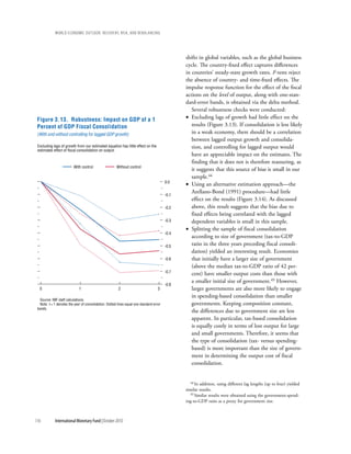
Will It Hurt? Macroeconomic Effects of Fiscal Consolidation October 2010, Chapter 3
Vi. Monetary policy, Financial Markets, and Flow of Funds
When Bubbles Burst April 2003, Chapter 2
How Do Balance Sheet Vulnerabilities Affect Investment? April 2003, Box 2.3
Identifying Asset Price Booms and Busts April 2003, Appendix 2.1
Are Foreign Exchange Reserves in Asia Too High? September 2003, Chapter 2
Reserves and Short-Term Debt September 2003, Box 2.3
Are Credit Booms in Emerging Markets a Concern? April 2004, Chapter 4
How Do U.S. Interest and Exchange Rates Affect Emerging Markets’
Balance Sheets? April 2004, Box 2.1
Does Financial Sector Development Help Economic Growth and Welfare? April 2004, Box 4.1
Adjustable- or Fixed-Rate Mortgages: What Influences a Country’s Choices? September 2004, Box 2.2
What Are the Risks from Low U.S. Long-Term Interest Rates? April 2005, Box 1.2
Regulating Remittances April 2005, Box 2.2
Financial Globalization and the Conduct of Macroeconomic Policies April 2005, Box 3.3
Monetary Policy in a Globalized World April 2005, Box 3.4
Does Inflation Targeting Work in Emerging Markets? September 2005, Chapter 4
A Closer Look at Inflation Targeting Alternatives: Money and
Exchange Rate Targets September 2005, Box 4.1
How Has Globalization Affected Inflation? April 2006, Chapter 3
The Impact of Petrodollars on U.S. and Emerging Market Bond Yields April 2006, Box 2.3
Globalization and Inflation in Emerging Markets April 2006, Box 3.1
Globalization and Low Inflation in a Historical Perspective April 2006, Box 3.2
Exchange Rate Pass-Through to Import Prices April 2006, Box 3.3
Trends in the Financial Sector’s Profits and Savings April 2006, Box 4.2
How Do Financial Systems Affect Economic Cycles? September 2006, Chapter 4
Financial Leverage and Debt Deflation September 2006, Box 4.1
Financial Linkages and Spillovers April 2007, Box 4.1
Macroeconomic Conditions in Industrial Countries and Financial Flows to
Emerging Markets April 2007, Box 4.2
What Is Global Liquidity? October 2007, Box 1.4
Macroeconomic Implications of Recent Market Turmoil: Patterns from
Previous Episodes October 2007, Box 1.2
The Changing Housing Cycle and the Implications for Monetary Policy April 2008, Chapter 3
Assessing Vulnerabilities to Housing Market Corrections April 2008, Box 3.1
Is There a Credit Crunch? April 2008, Box 1.1
International Monetary Fund | October 2010 213

232. Selected tOpicS
Financial Stress and Economic Downturns October 2008, Chapter 4
Policies to Resolve Financial System Stress and Restore
Sound Financial Intermediation October 2008, Box 4.1
The Latest Bout of Financial Distress: How Does It Change the Global Outlook? October 2008, Box 1.1
How Vulnerable Are Nonfinancial Firms? April 2009, Box 1.2
The Case of Vanishing Household Wealth April 2009, Box 2.1
Impact of Foreign Bank Ownership during Home-Grown Crises April 2009, Box 4.1
A Financial Stress Index for Emerging Economies April 2009, Appendix 4.1
Financial Stress in Emerging Economies: Econometric Analysis April 2009, Appendix 4.2
How Linkages Fuel the Fire April 2009, Chapter 4
Lessons for Monetary Policy from Asset Price Fluctuations October 2009, Chapter 3
Were Financial Markets in Emerging Economies More Resilient than in Past Crises? October 2009, Box 1.2
Risks from Real Estate Markets October 2009, Box 1.4
Vii. labor Markets, poverty, and inequality
Unemployment and Labor Market Institutions: Why Reforms Pay Off April 2003, Chapter 4
Regional Disparities in Unemployment April 2003, Box 4.1
Labor Market Reforms in the European Union April 2003, Box 4.2
The Globalization of Labor April 2007, Chapter 5
Emigration and Trade: How Do They Affect Developing Countries? April 2007, Box 5.1
Labor Market Reforms in the Euro Area and the Wage-Unemployment
Trade-Off October 2007, Box 2.2
Globalization and Inequality October 2007, Chapter 4
The Dualism between Temporary and Permanent Contracts: Measures,
Effects, and Policy Issues April 2010, Box 3.1
Short-Time Work Programs April 2010, Box 3.2
Viii. exchange Rate issues
The Pros and Cons of Dollarization May 2000, Box 1.4
Why Is the Euro So Undervalued? October 2000, Box 1.1
Convergence and Real Exchange Rate Appreciation in the EU
Accession Countries October 2000, Box 4.4
What Is Driving the Weakness of the Euro and the Strength of the Dollar? May 2001, Chapter 2
The Weakness of the Australian and New Zealand Currencies May 2001, Box 2.1
How Did the September 11 Attacks Affect Exchange Rate Expectations? December 2001, Box 2.4
Market Expectations of Exchange Rate Movements September 2002, Box 1.2
Are Foreign Exchange Reserves in Asia Too High? September 2003, Chapter 2
How Concerned Should Developing Countries Be about G-3
Exchange Rate Volatility? September 2003, Chapter 2
Reserves and Short-Term Debt September 2003, Box 2.3
The Effects of a Falling Dollar April 2004, Box 1.1
Learning to Float: The Experience of Emerging Market Countries since
the Early 1990s September 2004, Chapter 2
214 International Monetary Fund | October 2010

233. Selected tOpicS
How Did Chile, India, and Brazil Learn to Float? September 2004, Box 2.3
Foreign Exchange Market Development and Intervention September 2004, Box 2.4
How Emerging Market Countries May Be Affected by External Shocks September 2006, Box 1.3
Exchange Rates and the Adjustment of External Imbalances April 2007, Chapter 3
Exchange Rate Pass-Through to Trade Prices and External Adjustment April 2007, Box 3.3
Depreciation of the U.S. Dollar: Causes and Consequences April 2008, Box 1.2
Lessons from the Crisis: On the Choice of Exchange Rate Regime April 2010, Box 1.1
iX. external payments, trade, capital Movements, and Foreign debt
Risks to the Multilateral Trading System April 2004, Box 1.3
Is the Doha Round Back on Track? September 2004, Box 1.3
Regional Trade Agreements and Integration: The Experience with NAFTA September 2004, Box 1.4
Trade and Financial Integration in Europe: Five Years after the
Euro’s Introduction September 2004, Box 2.5
Globalization and External Imbalances April 2005, Chapter 3
The Ending of Global Textile Trade Quotas April 2005, Box 1.3
What Progress Has Been Made in Implementing Policies to Reduce
Global Imbalances? April 2005, Box 1.4
Measuring a Country’s Net External Position April 2005, Box 3.2
Global Imbalances: A Saving and Investment Perspective September 2005, Chapter 2
Impact of Demographic Change on Saving, Investment, and Current
Account Balances September 2005, Box 2.3
How Will Global Imbalances Adjust? September 2005,
Appendix 1.2
Oil Prices and Global Imbalances April 2006, Chapter 2
How Much Progress Has Been Made in Addressing Global Imbalances? April 2006, Box 1.4
The Doha Round after the Hong Kong SAR Meetings April 2006, Box 1.5
Capital Flows to Emerging Market Countries: A Long-Term Perspective September 2006, Box 1.1
How Will Global Imbalances Adjust? September 2006, Box 2.1
External Sustainability and Financial Integration April 2007, Box 3.1
Large and Persistent Current Account Imbalances April 2007, Box 3.2
Multilateral Consultation on Global Imbalances October 2007, Box 1.3
Managing the Macroeconomic Consequences of Large and Volatile Aid Flows October 2007, Box 2.3
Managing Large Capital Inflows October 2007, Chapter 3
Can Capital Controls Work? October 2007, Box 3.1
Multilateral Consultation on Global Imbalances: Progress Report April 2008, Box 1.3
How Does the Globalization of Trade and Finance Affect Growth?
Theory and Evidence April 2008, Box 5.1
Divergence of Current Account Balances across Emerging Economies October 2008, Chapter 6
Current Account Determinants for Oil-Exporting Countries October 2008, Box 6.1
Sovereign Wealth Funds: Implications for Global Financial Markets October 2008, Box 6.2
Global Imbalances and the Financial Crisis April 2009, Box 1.4
Trade Finance and Global Trade: New Evidence from Bank Surveys October 2009, Box 1.1
International Monetary Fund | October 2010 215

234. Selected tOpicS
From Deficit to Surplus: Recent Shifts in Global Current Accounts October 2009, Box 1.5
Getting the Balance Right: Transitioning out of Sustained Current Account Surpluses April 2010, Chapter 4
Emerging Asia: Responding to Capital Inflows October 2010, Box 2.1
Latin America-5: Riding Another Wave of Capital Inflows October 2010, Box 2.2
Do Financial Crises Have Lasting Effects on Trade? October 2010, Chapter 4
X. Regional issues
Promoting Stronger Institutions and Growth: The New Partnership for
Africa’s Development April 2003, Box 3.3
How Can Economic Growth in the Middle East and North Africa
Region Be Accelerated? September 2003, Chapter 2
Gulf Cooperation Council: Challenges on the Road to a Monetary Union September 2003, Box 1.5
Accounting for Growth in the Middle East and North Africa September 2003, Box 2.1
Is Emerging Asia Becoming an Engine of World Growth? April 2004, Box 1.4
What Works in Africa April 2004, Box 1.5
Economic Integration and Structural Reforms: The European Experience April 2004, Box 3.4
What Are the Risks of Slower Growth in China? September 2004, Box 1.2
Governance Challenges and Progress in Sub-Saharan Africa September 2004, Box 1.6
The Indian Ocean Tsunami: Impact on South Asian Economies April 2005, Box 1.1
Workers’ Remittances and Emigration in the Caribbean April 2005, Box 2.1
What Explains Divergent External Sector Performance in the Euro Area? September 2005, Box 1.3
Pressures Mount for African Cotton Producers September 2005, Box 1.5
Is Investment in Emerging Asia Too Low? September 2005, Box 2.4
Developing Institutions to Reflect Local Conditions: The Example of
Ownership Transformation in China versus Central and Eastern Europe September 2005, Box 3.1
How Rapidly Are Oil Exporters Spending Their Revenue Gains? April 2006, Box 2.1
EMU: 10 Years On October 2008, Box 2.1
Vulnerabilities in Emerging Economies April 2009, Box 2.2
Xi. country-Specific Analyses
How Important Are Banking Weaknesses in Explaining Germany’s Stagnation? April 2003, Box 1.3
Are Corporate Financial Conditions Related to the Severity of Recessions
in the United States? April 2003, Box 2.2
Rebuilding Post-Conflict Iraq September 2003, Box 1.4
How Will the U.S. Budget Deficit Affect the Rest of the World? April 2004, Chapter 2
China’s Emergence and Its Impact on the Global Economy April 2004, Chapter 2
Can China Sustain Its Rapid Output Growth? April 2004, Box 2.3
Quantifying the International Impact of China’s WTO Accession April 2004, Box 2.4
Structural Reforms and Economic Growth: New Zealand’s Experience April 2004, Box 3.1
Structural Reforms in the United Kingdom during the 1980s April 2004, Box 3.2
The Netherlands: How the Interaction of Labor Market Reforms and
Tax Cuts Led to Strong Employment Growth April 2004, Box 3.3
216 International Monetary Fund | October 2010

235. Selected tOpicS
Why Is the U.S. International Income Account Still in the Black,
and Will This Last? September, 2005, Box 1.2
Is India Becoming an Engine for Global Growth? September, 2005, Box 1.4
Saving and Investment in China September, 2005, Box 2.1
China’s GDP Revision: What Does It Mean for China and
the Global Economy? April 2006, Box 1.6
What Do Country Studies of the Impact of Globalization on Inequality Tell Us?
Examples from Mexico, China, and India October 2007, Box 4.2
Japan after the Plaza Accord April 2010, Box 4.1
Taiwan Province of China in the Late 1980s April 2010, Box 4.2
Xii. Special topics
Climate Change and the Global Economy April 2008, Chapter 4
Rising Car Ownership in Emerging Economies: Implications for Climate Change April 2008, Box 4.1
South Asia: Illustrative Impact of an Abrupt Climate Shock April 2008, Box 4.2
Macroeconomic Policies for Smoother Adjustment to Abrupt Climate Shocks April 2008, Box 4.3
Catastrophe Insurance and Bonds: New Instruments to Hedge Extreme
Weather Risks April 2008, Box 4.4
Recent Emission-Reduction Policy Initiatives April 2008, Box 4.5
Complexities in Designing Domestic Mitigation Policies April 2008, Box 4.6
International Monetary Fund | October 2010 217

237. Expand Your Global Expertise
Learn more about other macroeconomic reports available from the International Monetary Fund…
Global Financial Stability Report
The GFSR aims to deepen understanding of global capital flows, which play
a critical role as an engine of world economic growth. It focuses on current
conditions in global financial markets, highlighting issues of both financial
imbalances and of a structural nature that could pose risks to financial market
stability and market access. The GFSR also draws out the financial ramifications
of economic imbalances highlighted by the World Economic Outlook, making it
an indispensable companion publication.
Annual subscription: $108. Paperback
Published twice yearly. ISSN: 1729-701X. Stock# GFSREA
Fiscal Monitor
A key aspect of the IMF’s surveillance responsibilities has gained further importance with
increasing fiscal challenges in the aftermath of the global financial crisis and multilateral
surveillance of fiscal developments. The Fiscal Monitor was launched in 2009 to survey
and analyze the latest public finance developments, update fiscal implications of the
crisis and medium-term fiscal projections, and assess policies to put public finances on
a sustainable footing. The Fiscal Monitor is prepared twice a year by the IMF’s Fiscal
Affairs Department. The Monitor’s projections are based on the same database used for
the World Economic Outlook and Global Financial Stability Report.
English. Paperback. Individual issues of the Fiscal Monitor are available at $35
(academic rate: $30).
Annual subscription $53. Published twice yearly. ISSN: 2219-276X. Stock# FMOEA2010002
Regional Economic
Outlooks
How do prudent economic
policies help regions absorb
potential shocks and spillovers
from one economy to another? In
this environment, the International
Monetary Fund’s five Regional
Economic Outlooks are more
valuable than ever. Recent economic developments and prospects are d
d discussed for the region as a whole as well as for
d
specific economies. The reports include key data for economies that make up each region as well as surveys of regional
economic and financial development and trends.
Individual copies of the Regional Economic Outlooks are available for $35 (academic rate: $30).
For detailed information or to place an order, please go to www.imfbookstore.org or contact publications@imf.org.