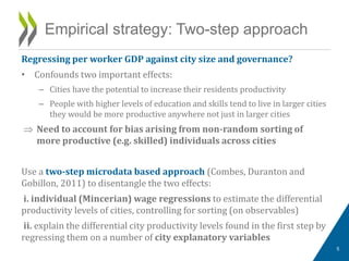
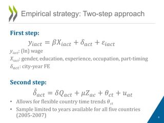
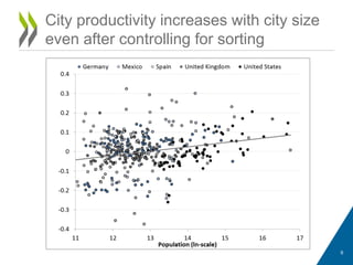
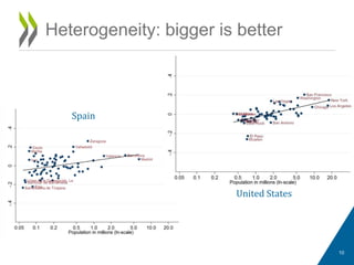
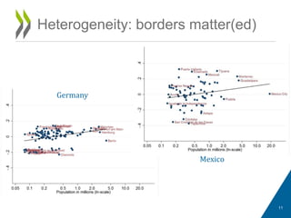
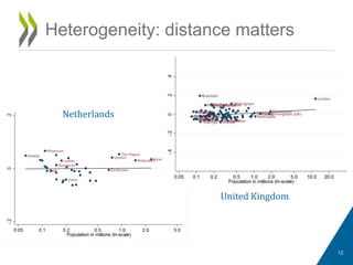
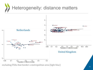
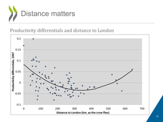
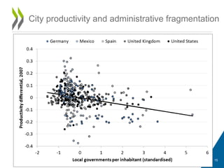
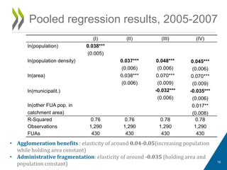
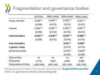
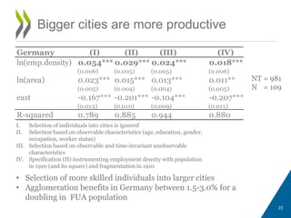
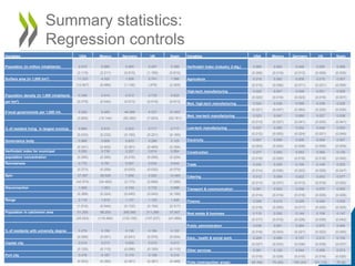
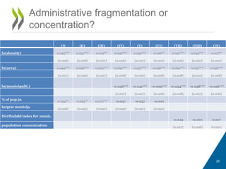
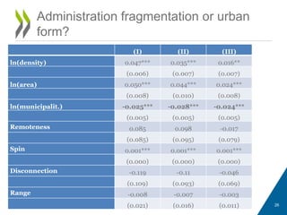
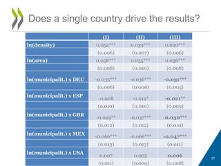
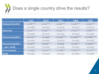
Rudiger Ahrend and Alexander C. Lembcke
OECD/GOV, Regional Development Policy Division
OECD, 15 January 2015
What Makes Cities More Productive?
Agglomeration economies and
the role of urban governance
What determines productivity in cities?
• Focus on cities’ size and their governance structures
Evidence for 5 (+2) OECD countries:
• Germany, Mexico, Spain, UK and US
• Netherlands and Japan in progress
Coherent and comparative methodology
• Use wage microdata and OECD Functional Urban Areas:
Economic links (commuting flows) define a city’s
boundary rather than the city’s administrative limits
• Two-step econometric framework  account for
individual characteristics that determine productivity
Preliminaries: what, who and how?
2
Sources of agglomeration economies
Reviews by Rosenthal and Strange (2004), Duranton and Puga (2004) and
Puga (2010); concepts already present in Marshall (1890).
• Sharing facilities, inputs, gains from specialisation
firms may face lower costs for specialised non-traded inputs that are
shared locally in a geographical cluster.
• Thicker labour markets: labour market pooling; better matching
gain from reduced labour acquisition and training costs in thick local
labour markets with abundant specialised labour force
• Knowledge spillovers: learning about and spreading new ideas
face-to-face contact can enable tacit knowledge spillovers through
increases in the intensity of the interactions with other firms or
individuals
Agglomeration economies
3
Horizontal administrative fragmentation is common as cities
outgrow their historic boundaries (more than 10 local governments
in 75% of OECD Metropolitan Areas; more than 100 in 22%)
Potential positive impact:
• a larger number of local governments is associated with more choice in the
provision of public services, more tailored solutions and better
accountability (Tiebout, 1956).
• Large literature that finds no scale effects for specific public services
(Ostrom, 2010) or governmental expenditure (Kalb, 2010).
Potential negative impact:
• Policies, investment and services require city-wide coordination (e.g.
Cheshire and Gordon, 1996): e.g. transport; land use; ease of doing business;
economic promotion; environmental regulation, etc.
Fragmentation and governance
4
Regressing per worker GDP against city size and governance?
• Confounds two important effects:
– Cities have the potential to increase their residents productivity
– People with higher levels of education and skills tend to live in larger cities
they would be more productive anywhere not just in larger cities
⇒ Need to account for bias arising from non-random sorting of
more productive (e.g. skilled) individuals across cities
Use a two-step microdata based approach (Combes, Duranton and
Gobillon, 2011) to disentangle the two effects:
i. individual (Mincerian) wage regressions to estimate the differential
productivity levels of cities, controlling for sorting (on observables)
ii. explain the differential city productivity levels found in the first step by
regressing them on a number of city explanatory variables
Empirical strategy: Two-step approach
5
First step:
𝑦𝑖𝑖𝑐𝑡 = 𝛽𝑋𝑖𝑖𝑐𝑡 + 𝛿 𝑎𝑎𝑡 + 𝜀𝑖𝑖𝑐𝑡
yiact: (ln) wage
Xiact: gender, education, experience, occupation, part-timing
𝛿 𝑎𝑐𝑡: city-year FE
Second step:
𝛿̂ 𝑎𝑐𝑡 = 𝛿𝑄 𝑎𝑐𝑡 + 𝜇𝑍 𝑎𝑐 + 𝜃𝑐𝑡 + 𝑢 𝑎𝑎
• Allows for flexible country time trends 𝜃ct
• Sample limited to years available for all five countries
(2005-2007)
Empirical strategy: Two-step approach
6
Explain first stage estimates with a set of relevant city
(Functional Urban Area) level controls (𝑄 𝑎𝑐𝑡; 𝑍 𝑎𝑐)
• agglomeration: (ln) population density and (ln) area
• urban governance: horizontal administrative
fragmentation (ln number of municipalities; presence of
a governance body; interaction term)
• human capital: share of university graduates
• industrial structure: specialisation, composition and
technological intensity
• location “fundamentals”: port; capital city; pop in
cities within 300km radius
• urban form: population concentration; complexity of
the shape of the urban built-up area
Empirical strategy: City characteristics
7
Microdata with info on wages, individual characteristics
and detailed residence/workplace location
• UK: ASHE first stage (1% sample); city-year controls from QLFS;
2004-2010
• Spain: MCVL; administrative data (4% sample); 2005-2011
• Germany: BA-Employment Panel (2% sample, 1998-2007)
• US: IPUMS data; Census 1990, 2000 and American Community
Survey 2005-2007
• Mexico: ENE 2000-2004; ENOE 2005-2010
• Japan: Basic Survey on Wage Structure (~3% of employees,
1989-2013)
• Netherlands: Census (SSB); Labour Force Survey (EBB); Firm
registry (EBB) for 2010
Data
8
City productivity increases with city size
even after controlling for sorting
9
Heterogeneity: bigger is better
10
Spain
United States
Heterogeneity: borders matter(ed)
11
Germany
Mexico
Heterogeneity: distance matters
12
Netherlands
United Kingdom
Netherlands
Heterogeneity: distance matters
13
excluding FUAs that border a metropolitan area (light blue)
United Kingdom
Distance matters
14
Productivity differentials and distance to London
City productivity and administrative fragmentation
15
Pooled regression results, 2005-2007
16
(I) (II) (III) (IV)
ln(population) 0.038***
(0.005)
ln(population density) 0.037*** 0.048*** 0.045***
(0.006) (0.006) (0.006)
ln(area) 0.038*** 0.070*** 0.070***
(0.006) (0.009) (0.009)
ln(municipalit.) -0.032*** -0.035***
(0.006) (0.006)
ln(other FUA pop. in 0.017**
catchment area) (0.008)
R-Squared 0.76 0.76 0.78 0.78
Observations 1,290 1,290 1,290 1,290
FUAs 430 430 430 430
• Agglomeration benefits : elasticity of around 0.04-0.05(increasing population
while holding area constant)
• Administrative fragmentation: elasticity of around -0.035 (holding area and
population constant)
All FUAs Metro areas Metro areas Metro areas
ln(pop. density) 0.048*** 0.064*** 0.065*** 0.047***
(0.006) (0.012) (0.012) (0.012)
ln(area) 0.064*** 0.082*** 0.085*** 0.087***
(0.008) (0.012) (0.012) (0.013)
ln(municipalit.) -0.032*** -0.032*** -0.057*** -0.066***
(0.006) (0.010) (0.016) (0.017)
ln(municipalit.) 0.031** 0.036**
x govern. body (0.014) (0.015)
governance body -0.079** -0.092**
(0.034) (0.038)
Add.controls no no no yes
R-Squared 0.779 0.847 0.855 0.880
Observations (FUAs) 1,290 (430) 420 (140) 420 (140) 420 (140)
Fragmentation and governance bodies
17
Taking governance bodies into account shows the true fragmentation penalty:
-0.06 with governance bodies attenuating half.
Human capital, high-tech and knowledge intensive
services oriented cities make their residents more
productive
Smaller cities can
“borrow”
agglomeration
benefits
Benefits are not
limited to cities
but positively affect
accessible regions
Beyond city size and governance
18
Ahrend and Schumann (2014)
Annual per capita GDP growth rates (1995-2010) and driving time to the
closest metro area of 2 million or more inhabitants
• First study that quantifies link between (horizontal)
administrative fragmentation, the role of governance bodies
and productivity in cities, using a comparable and coherent
definition for “cities” and a common empirical strategy.
• Size matters: Estimated elasticity for agglomeration benefits
around 0.02-0.05 (roughly: 2-5% higher productivity for a
doubling in population)
• Cities with fragmented governance structures exhibit lower
levels of productivity:
Doubling the number of municipalities within a metropolitan
area is associated with 6% lower productivity
=> The presence of a governance body halves this penalty
• Productivity is higher in cities with more skilled workers; with
larger employment shares in high-tech manufacturing,
finance and business services; larger neighbouring cities and
lower levels of governmental fragmentation.
City productivity:
Results from 5 OECD countries
19
The presentation draws from:
Ahrend, Farchy, Kaplanis and Lembcke (2014)
“What Makes Cities More Productive?
Agglomeration economies and the role of urban
governance: Evidence from 5 OECD Countries”
Ahrend and Schumann (2014) “Does regional economic growth
depend on proximity to urban centres?”
OECD (2015) The Metropolitan Century: Understanding Urbanisation and its
Consequences
OECD (2015) Governing the City
OECD (forthcoming) Metropolitan Review: Rotterdam-The Hague
OECD (2012) Redefining Urban: a new way to measure metropolitan areas
Thank you
20
Local productivity, prices and
purchasing power
21
What explains the heterogeneity in net
differentials?
Germany (1999-2007) West Germany (1999-2007)
(L) (M) (N) (O) (L) (M) (N) (O)
Access to coast or -0.012* -0.006 -0.014** -0.005 -0.011 -0.003 -0.012* -0.003
large lake (0.007) (0.007) (0.006) (0.007) (0.008) (0.008) (0.007) (0.008)
UNESCO cultural -0.009* -0.009 -0.008* -0.008* -0.012** -0.013** -0.011** -0.013***
heritage site (0.005) (0.005) (0.005) (0.005) (0.006) (0.006) (0.005) (0.005)
Number of theatre -0.014*** -0.017*** -0.010** -0.010*** -0.015** -0.019** -0.007 -0.008
seats / 1,000 (0.005) (0.005) (0.004) (0.004) (0.007) (0.008) (0.005) (0.005)
Number of theatre 0.001*** 0.001*** 0.001*** 0.001*** 0.001 0.001* 0.000 0.000
seats / 1,000 (sq.) (0.000) (0.000) (0.000) (0.000) (0.001) (0.001) (0.001) (0.001)
University hospital in -0.001 0.000 -0.007 -0.000 -0.004 -0.001 -0.007 0.001
FUA (0.006) (0.007) (0.005) (0.006) (0.006) (0.007) (0.005) (0.006)
Number of universities -0.007*** -0.007*** -0.002 -0.002 -0.008*** -0.009*** -0.004** -0.004**
(0.002) (0.002) (0.001) (0.001) (0.002) (0.003) (0.002) (0.002)
Numb. of nat. league 0.001 0.000 -0.002 -0.003 0.002 0.002 0.000 0.000
football clubs 1995-99 (0.006) (0.006) (0.004) (0.004) (0.006) (0.007) (0.004) (0.004)
Avg. annual level of 0.005** 0.004** 0.003 0.002*
PM10 (0.002) (0.002) (0.002) (0.001)
Share of workers w/ -0.315*** -0.254*** -0.379*** -0.323*** -0.322*** -0.267*** -0.345*** -0.264***
university degree (0.087) (0.085) (0.077) (0.083) (0.088) (0.084) (0.073) (0.066)
R-squared 0.45 0.46 0.39 0.39 0.50 0.54 0.33 0.35
FUAs 109 100 109 100 88 80 88 80
Obs. 981 541 981 541 792 423 792 423
Productivity indicators Aggl. Aggl. All All Aggl. Aggl. All All
22
Bigger cities are more productive
Germany (I) (II) (III) (IV)
ln(emp.density) 0.054*** 0.029*** 0.024*** 0.018***
(0.006) (0.005) (0.005) (0.006)
ln(area) 0.023*** 0.015*** 0.013*** 0.011**
(0.005) (0.004) (0.004) (0.005)
east -0.167*** -0.201*** -0.104*** -0.207***
(0.012) (0.010) (0.009) (0.011)
R-squared 0.789 0.885 0.944 0.880
NT = 981
NT = 109
I. Selection of individuals into cities is ignored
II. Selection based on observable characteristics (age, education, gender,
occupation, worker status)
III. Selection based on observable and time-invariant unobservable
characteristics
IV. Specification (II) instrumenting employment density with population
in 1910 (and its square) and fragmentation in 1910
• Selection of more skilled individuals into larger cities
• Agglomeration benefits in Germany between 1.5-3.0% for a
doubling in FUA population
23
Summary statistics:
Regression controls
24
Variables USA Mexico Germany UK Spain
Population (in million inhabitants) 2.470 0.880 0.465 0.457 0.389
(3.115) (2.211) (0.615) (1.169) (0.810)
Surface area (in 1,000 km²) 11.233 4.322 1.208 0.741 1.566
(12.907) (6.989) (1.136) (.878) (2.205)
Population density (in 1,000 inhabitants 0.349 0.414 0.512 0.735 0.625
per km²) (0.379) (0.542) (0.513) (0.518) (0.913)
# local governments per 1,000 inh. 5.000 5.400 44.266 4.337 31.803
(3.800) (10.144) (50.390) (7.003) (52.161)
% of resident living in largest municip. 0.665 0.810 0.522 0.717 0.717
(0.233) (0.232) (0.183) (0.221) (0.165)
Governance body 0.868 0.808 0.833 0.286 0.125
(0.341) (0.402) (0.381) (0.469) (0.354)
Herfindahl index for municipal 0.550 0.739 0.327 0.614 0.564
population concentration (0.265) (0.295) (0.216) (0.256) (0.224)
Remoteness 0.770 0.781 0.547 0.534 0.645
(0.273) (0.258) (0.033) (0.032) (0.079)
Spin 37.597 26.929 7.958 5.920 10.465
(42.574) (34.460) (3.173) (2.699) (7.288)
Disconnection 1.065 1.063 0.749 0.732 0.888
(0.388) (0.324) (0.045) (0.043) (0.106)
Range 2.116 1.819 1.137 1.125 1.455
(1.610) (0.944) (0.132) (0.154) (0.317)
Population in catchment area 51,305 88,200 265,560 311,389 57,607
(45,524) (119,364) (133,150) (107,237) (41,566)
% of residents with university degree 0.276 0.156 0.136 0.194 0.122
(0.056) (0.051) (0.041) (0.070) (0.054)
Capital city 0.014 0.013 0.009 0.010 0.013
(0.120) (0.115) (0.096) (0.100) (0.115)
Port city 0.478 0.187 0.174 0.158 0.316
(0.503) (0.392) (0.381) (0.367) (0.468)
Variables USA Mexico Germany UK Spain
Herfindahl Index (industry 2-dig.) 0.060 0.063 0.046 0.050 0.068
(0.006) (0.018) (0.013) (0.009) (0.025)
Agriculture 0.018 0.062 0.008 0.015 0.007
(0.015) (0.056) (0.011) (0.021) (0.006)
High-tech manufacturing 0.022 0.007 0.026 0.021 0.005
(0.020) (0.016) (0.023) (0.016) (0.007)
Med. high-tech manufacturing 0.024 0.036 0.095 0.039 0.026
(0.021) (0.047) (0.064) (0.020) (0.030)
Med. low-tech manufacturing 0.023 0.047 0.060 0.037 0.038
(0.013) (0.027) (0.041) (0.020) (0.041)
Low-tech manufacturing 0.037 0.080 0.052 0.046 0.052
(0.012) (0.055) (0.024) (0.021) (0.049)
Electricity 0.007 0.006 0.005 0.009 0.007
(0.003) (0.004) (0.008) (0.006) (0.005)
Construction 0.077 0.093 0.053 0.084 0.130
(0.016) (0.026) (0.016) (0.018) (0.042)
Trade 0.220 0.209 0.150 0.149 0.203
(0.014) (0.036) (0.022) (0.028) (0.047)
Catering 0.012 0.069 0.022 0.043 0.077
(0.013) (0.037) (0.013) (0.016) (0.052)
Transport & communication 0.061 0.053 0.058 0.070 0.055
(0.014) (0.019) (0.019) (0.029) (0.026)
Finance 0.056 0.010 0.029 0.040 0.035
(0.018) (0.006) (0.017) (0.020) (0.025)
Real estate & business 0.115 0.050 0.144 0.109 0.147
(0.017) (0.018) (0.028) (0.036) (0.042)
Public administration 0.038 0.061 0.064 0.070 0.045
(0.016) (0.043) (0.021) (0.022) (0.040)
Educ., health & social work 0.209 0.099 0.157 0.213 0.102
(0.027) (0.033) (0.036) (0.039) (0.037)
Other services 0.081 0.120 0.044 0.056 0.073
(0.016) (0.028) (0.015) (0.016) (0.020)
FUAs (metropolitan areas) 69 (68) 75 (26) 109 (24) 101 (14) 76 (8)
(I) (II) (III) (IV) (V) (VI) (VII) (VIII) (IX)
ln(density) 0.043*** 0.031*** 0.015** 0.046*** 0.032*** 0.016** 0.047*** 0.034*** 0.017**
(0.006) (0.008) (0.007) (0.006) (0.007) (0.007) (0.006) (0.007) (0.007)
ln(area) 0.044*** 0.036*** 0.022*** 0.064*** 0.057*** 0.036*** 0.064*** 0.057*** 0.036***
(0.007) (0.009) (0.007) (0.008) (0.010) (0.008) (0.008) (0.010) (0.008)
ln(municipalit.) -0.036*** -0.041*** -0.029*** -0.034*** -0.038*** -0.026***
(0.007) (0.007) (0.006) (0.008) (0.007) (0.006)
% of pop.in 0.054** 0.063** 0.072*** -0.037 -0.037 -0.001
largest municip. (0.026) (0.025) (0.021) (0.029) (0.027) (0.022)
Herfindahl index for munic.
-0.013 -0.010 0.017
population concentration (0.027) (0.026) (0.021)
Administrative fragmentation or
concentration?
25
(I) (II) (III)
ln(density) 0.047*** 0.035*** 0.016**
(0.006) (0.007) (0.007)
ln(area) 0.050*** 0.044*** 0.024***
(0.008) (0.010) (0.008)
ln(municipalit.) -0.025*** -0.028*** -0.024***
(0.005) (0.005) (0.005)
Remoteness 0.085 0.098 -0.017
(0.085) (0.095) (0.079)
Spin 0.001*** 0.001*** 0.001***
(0.000) (0.000) (0.000)
Disconnection -0.119 -0.11 -0.046
(0.109) (0.093) (0.069)
Range -0.008 -0.007 -0.003
(0.021) (0.016) (0.011)
Administration fragmentation or urban
form?
26
(I) (II) (III)
ln(density) 0.052*** 0.039*** 0.020***
(0.006) (0.007) (0.006)
ln(area) 0.058*** 0.055*** 0.036***
(0.008) (0.010) (0.008)
ln(municipalit.) x DEU -0.035*** -0.036*** -0.031***
(0.006) (0.006) (0.005)
ln(municipalit.) x ESP
-0.008 -0.019* -0.021**
(0.010) (0.010) (0.009)
ln(municipalit.) x GBR
-0.029** -0.037*** -0.030***
(0.012) (0.012) (0.010)
ln(municipalit.) x MEX
-0.066*** -0.066*** -0.047***
(0.013) (0.013) (0.011)
ln(municipalit.) x USA
0.007 0.005 0.006
(0.011) (0.009) (0.008)
Does a single country drive the results?
27
USA MEX DEU GBR ESP
ln(pop.density) 0.068*** 0.037*** 0.048*** 0.048*** 0.055***
(0.028) (0.010) (0.012) (0.012) (0.011)
ln(area) 0.140*** 0.059*** 0.092*** 0.092*** 0.088***
(0.026) (0.011) (0.014) (0.013) (0.013)
ln(municipalit.) -0.075*** -0.032* -0.052*** -0.066*** -0.080***
(0.022) (0.020) (0.021) (0.019) (0.016)
ln(municipalit.) 0.027* 0.031** 0.024 0.037** 0.049***
× gov. body (0.020) (0.016) (0.019) (0.016) (0.015)
Governance -0.054 -0.070** -0.084** -0.092*** -0.111***
body (0.055) (0.042) (0.041) (0.039) (0.036)
Does a single country drive the results?
28
% university 0.275***
Graduates (0.073)
Capital 0.028
(0.030)
Port 0.039***
(0.010)
Herfindahl -0.704***
Index (0.266)
Agriculture 0.0808
(0.257)
Catering 0.472**
(0.230)
Other determinants
29
Transport & -0.126
communication (0.200)
Finance 0.878***
(0.181)
Real estate 0.410**
& business (0.176)
Public 0.057
administration (0.261)
Educ., health -0.120
& social work (0.154)
Other services 0.535*
(0.275)
High-tech 1.104***
Manufacturin
g (0.234)
Med. high-
tech 0.840***
Manufacturin
g (0.135)
Med. low-
tech 0.494***
Manufacturin
g (0.146)
Low-tech 0.082
Manufacturin
g (0.149)
Electricity -0.931**
(0.463)
Trade 0.223
(0.171)

What makes cities more productive?

  • 1.
    Rudiger Ahrend andAlexander C. Lembcke OECD/GOV, Regional Development Policy Division OECD, 15 January 2015 What Makes Cities More Productive? Agglomeration economies and the role of urban governance
  • 2.
    What determines productivityin cities? • Focus on cities’ size and their governance structures Evidence for 5 (+2) OECD countries: • Germany, Mexico, Spain, UK and US • Netherlands and Japan in progress Coherent and comparative methodology • Use wage microdata and OECD Functional Urban Areas: Economic links (commuting flows) define a city’s boundary rather than the city’s administrative limits • Two-step econometric framework  account for individual characteristics that determine productivity Preliminaries: what, who and how? 2
  • 3.
    Sources of agglomerationeconomies Reviews by Rosenthal and Strange (2004), Duranton and Puga (2004) and Puga (2010); concepts already present in Marshall (1890). • Sharing facilities, inputs, gains from specialisation firms may face lower costs for specialised non-traded inputs that are shared locally in a geographical cluster. • Thicker labour markets: labour market pooling; better matching gain from reduced labour acquisition and training costs in thick local labour markets with abundant specialised labour force • Knowledge spillovers: learning about and spreading new ideas face-to-face contact can enable tacit knowledge spillovers through increases in the intensity of the interactions with other firms or individuals Agglomeration economies 3
  • 4.
    Horizontal administrative fragmentationis common as cities outgrow their historic boundaries (more than 10 local governments in 75% of OECD Metropolitan Areas; more than 100 in 22%) Potential positive impact: • a larger number of local governments is associated with more choice in the provision of public services, more tailored solutions and better accountability (Tiebout, 1956). • Large literature that finds no scale effects for specific public services (Ostrom, 2010) or governmental expenditure (Kalb, 2010). Potential negative impact: • Policies, investment and services require city-wide coordination (e.g. Cheshire and Gordon, 1996): e.g. transport; land use; ease of doing business; economic promotion; environmental regulation, etc. Fragmentation and governance 4
  • 5.
    Regressing per workerGDP against city size and governance? • Confounds two important effects: – Cities have the potential to increase their residents productivity – People with higher levels of education and skills tend to live in larger cities they would be more productive anywhere not just in larger cities ⇒ Need to account for bias arising from non-random sorting of more productive (e.g. skilled) individuals across cities Use a two-step microdata based approach (Combes, Duranton and Gobillon, 2011) to disentangle the two effects: i. individual (Mincerian) wage regressions to estimate the differential productivity levels of cities, controlling for sorting (on observables) ii. explain the differential city productivity levels found in the first step by regressing them on a number of city explanatory variables Empirical strategy: Two-step approach 5
  • 6.
    First step: 𝑦𝑖𝑖𝑐𝑡 =𝛽𝑋𝑖𝑖𝑐𝑡 + 𝛿 𝑎𝑎𝑡 + 𝜀𝑖𝑖𝑐𝑡 yiact: (ln) wage Xiact: gender, education, experience, occupation, part-timing 𝛿 𝑎𝑐𝑡: city-year FE Second step: 𝛿̂ 𝑎𝑐𝑡 = 𝛿𝑄 𝑎𝑐𝑡 + 𝜇𝑍 𝑎𝑐 + 𝜃𝑐𝑡 + 𝑢 𝑎𝑎 • Allows for flexible country time trends 𝜃ct • Sample limited to years available for all five countries (2005-2007) Empirical strategy: Two-step approach 6
  • 7.
    Explain first stageestimates with a set of relevant city (Functional Urban Area) level controls (𝑄 𝑎𝑐𝑡; 𝑍 𝑎𝑐) • agglomeration: (ln) population density and (ln) area • urban governance: horizontal administrative fragmentation (ln number of municipalities; presence of a governance body; interaction term) • human capital: share of university graduates • industrial structure: specialisation, composition and technological intensity • location “fundamentals”: port; capital city; pop in cities within 300km radius • urban form: population concentration; complexity of the shape of the urban built-up area Empirical strategy: City characteristics 7
  • 8.
    Microdata with infoon wages, individual characteristics and detailed residence/workplace location • UK: ASHE first stage (1% sample); city-year controls from QLFS; 2004-2010 • Spain: MCVL; administrative data (4% sample); 2005-2011 • Germany: BA-Employment Panel (2% sample, 1998-2007) • US: IPUMS data; Census 1990, 2000 and American Community Survey 2005-2007 • Mexico: ENE 2000-2004; ENOE 2005-2010 • Japan: Basic Survey on Wage Structure (~3% of employees, 1989-2013) • Netherlands: Census (SSB); Labour Force Survey (EBB); Firm registry (EBB) for 2010 Data 8
  • 9.
    City productivity increaseswith city size even after controlling for sorting 9
  • 10.
    Heterogeneity: bigger isbetter 10 Spain United States
  • 11.
  • 12.
  • 13.
    Netherlands Heterogeneity: distance matters 13 excludingFUAs that border a metropolitan area (light blue) United Kingdom
  • 14.
  • 15.
    City productivity andadministrative fragmentation 15
  • 16.
    Pooled regression results,2005-2007 16 (I) (II) (III) (IV) ln(population) 0.038*** (0.005) ln(population density) 0.037*** 0.048*** 0.045*** (0.006) (0.006) (0.006) ln(area) 0.038*** 0.070*** 0.070*** (0.006) (0.009) (0.009) ln(municipalit.) -0.032*** -0.035*** (0.006) (0.006) ln(other FUA pop. in 0.017** catchment area) (0.008) R-Squared 0.76 0.76 0.78 0.78 Observations 1,290 1,290 1,290 1,290 FUAs 430 430 430 430 • Agglomeration benefits : elasticity of around 0.04-0.05(increasing population while holding area constant) • Administrative fragmentation: elasticity of around -0.035 (holding area and population constant)
  • 17.
    All FUAs Metroareas Metro areas Metro areas ln(pop. density) 0.048*** 0.064*** 0.065*** 0.047*** (0.006) (0.012) (0.012) (0.012) ln(area) 0.064*** 0.082*** 0.085*** 0.087*** (0.008) (0.012) (0.012) (0.013) ln(municipalit.) -0.032*** -0.032*** -0.057*** -0.066*** (0.006) (0.010) (0.016) (0.017) ln(municipalit.) 0.031** 0.036** x govern. body (0.014) (0.015) governance body -0.079** -0.092** (0.034) (0.038) Add.controls no no no yes R-Squared 0.779 0.847 0.855 0.880 Observations (FUAs) 1,290 (430) 420 (140) 420 (140) 420 (140) Fragmentation and governance bodies 17 Taking governance bodies into account shows the true fragmentation penalty: -0.06 with governance bodies attenuating half.
  • 18.
    Human capital, high-techand knowledge intensive services oriented cities make their residents more productive Smaller cities can “borrow” agglomeration benefits Benefits are not limited to cities but positively affect accessible regions Beyond city size and governance 18 Ahrend and Schumann (2014) Annual per capita GDP growth rates (1995-2010) and driving time to the closest metro area of 2 million or more inhabitants
  • 19.
    • First studythat quantifies link between (horizontal) administrative fragmentation, the role of governance bodies and productivity in cities, using a comparable and coherent definition for “cities” and a common empirical strategy. • Size matters: Estimated elasticity for agglomeration benefits around 0.02-0.05 (roughly: 2-5% higher productivity for a doubling in population) • Cities with fragmented governance structures exhibit lower levels of productivity: Doubling the number of municipalities within a metropolitan area is associated with 6% lower productivity => The presence of a governance body halves this penalty • Productivity is higher in cities with more skilled workers; with larger employment shares in high-tech manufacturing, finance and business services; larger neighbouring cities and lower levels of governmental fragmentation. City productivity: Results from 5 OECD countries 19
  • 20.
    The presentation drawsfrom: Ahrend, Farchy, Kaplanis and Lembcke (2014) “What Makes Cities More Productive? Agglomeration economies and the role of urban governance: Evidence from 5 OECD Countries” Ahrend and Schumann (2014) “Does regional economic growth depend on proximity to urban centres?” OECD (2015) The Metropolitan Century: Understanding Urbanisation and its Consequences OECD (2015) Governing the City OECD (forthcoming) Metropolitan Review: Rotterdam-The Hague OECD (2012) Redefining Urban: a new way to measure metropolitan areas Thank you 20
  • 21.
    Local productivity, pricesand purchasing power 21
  • 22.
    What explains theheterogeneity in net differentials? Germany (1999-2007) West Germany (1999-2007) (L) (M) (N) (O) (L) (M) (N) (O) Access to coast or -0.012* -0.006 -0.014** -0.005 -0.011 -0.003 -0.012* -0.003 large lake (0.007) (0.007) (0.006) (0.007) (0.008) (0.008) (0.007) (0.008) UNESCO cultural -0.009* -0.009 -0.008* -0.008* -0.012** -0.013** -0.011** -0.013*** heritage site (0.005) (0.005) (0.005) (0.005) (0.006) (0.006) (0.005) (0.005) Number of theatre -0.014*** -0.017*** -0.010** -0.010*** -0.015** -0.019** -0.007 -0.008 seats / 1,000 (0.005) (0.005) (0.004) (0.004) (0.007) (0.008) (0.005) (0.005) Number of theatre 0.001*** 0.001*** 0.001*** 0.001*** 0.001 0.001* 0.000 0.000 seats / 1,000 (sq.) (0.000) (0.000) (0.000) (0.000) (0.001) (0.001) (0.001) (0.001) University hospital in -0.001 0.000 -0.007 -0.000 -0.004 -0.001 -0.007 0.001 FUA (0.006) (0.007) (0.005) (0.006) (0.006) (0.007) (0.005) (0.006) Number of universities -0.007*** -0.007*** -0.002 -0.002 -0.008*** -0.009*** -0.004** -0.004** (0.002) (0.002) (0.001) (0.001) (0.002) (0.003) (0.002) (0.002) Numb. of nat. league 0.001 0.000 -0.002 -0.003 0.002 0.002 0.000 0.000 football clubs 1995-99 (0.006) (0.006) (0.004) (0.004) (0.006) (0.007) (0.004) (0.004) Avg. annual level of 0.005** 0.004** 0.003 0.002* PM10 (0.002) (0.002) (0.002) (0.001) Share of workers w/ -0.315*** -0.254*** -0.379*** -0.323*** -0.322*** -0.267*** -0.345*** -0.264*** university degree (0.087) (0.085) (0.077) (0.083) (0.088) (0.084) (0.073) (0.066) R-squared 0.45 0.46 0.39 0.39 0.50 0.54 0.33 0.35 FUAs 109 100 109 100 88 80 88 80 Obs. 981 541 981 541 792 423 792 423 Productivity indicators Aggl. Aggl. All All Aggl. Aggl. All All 22
  • 23.
    Bigger cities aremore productive Germany (I) (II) (III) (IV) ln(emp.density) 0.054*** 0.029*** 0.024*** 0.018*** (0.006) (0.005) (0.005) (0.006) ln(area) 0.023*** 0.015*** 0.013*** 0.011** (0.005) (0.004) (0.004) (0.005) east -0.167*** -0.201*** -0.104*** -0.207*** (0.012) (0.010) (0.009) (0.011) R-squared 0.789 0.885 0.944 0.880 NT = 981 NT = 109 I. Selection of individuals into cities is ignored II. Selection based on observable characteristics (age, education, gender, occupation, worker status) III. Selection based on observable and time-invariant unobservable characteristics IV. Specification (II) instrumenting employment density with population in 1910 (and its square) and fragmentation in 1910 • Selection of more skilled individuals into larger cities • Agglomeration benefits in Germany between 1.5-3.0% for a doubling in FUA population 23
  • 24.
    Summary statistics: Regression controls 24 VariablesUSA Mexico Germany UK Spain Population (in million inhabitants) 2.470 0.880 0.465 0.457 0.389 (3.115) (2.211) (0.615) (1.169) (0.810) Surface area (in 1,000 km²) 11.233 4.322 1.208 0.741 1.566 (12.907) (6.989) (1.136) (.878) (2.205) Population density (in 1,000 inhabitants 0.349 0.414 0.512 0.735 0.625 per km²) (0.379) (0.542) (0.513) (0.518) (0.913) # local governments per 1,000 inh. 5.000 5.400 44.266 4.337 31.803 (3.800) (10.144) (50.390) (7.003) (52.161) % of resident living in largest municip. 0.665 0.810 0.522 0.717 0.717 (0.233) (0.232) (0.183) (0.221) (0.165) Governance body 0.868 0.808 0.833 0.286 0.125 (0.341) (0.402) (0.381) (0.469) (0.354) Herfindahl index for municipal 0.550 0.739 0.327 0.614 0.564 population concentration (0.265) (0.295) (0.216) (0.256) (0.224) Remoteness 0.770 0.781 0.547 0.534 0.645 (0.273) (0.258) (0.033) (0.032) (0.079) Spin 37.597 26.929 7.958 5.920 10.465 (42.574) (34.460) (3.173) (2.699) (7.288) Disconnection 1.065 1.063 0.749 0.732 0.888 (0.388) (0.324) (0.045) (0.043) (0.106) Range 2.116 1.819 1.137 1.125 1.455 (1.610) (0.944) (0.132) (0.154) (0.317) Population in catchment area 51,305 88,200 265,560 311,389 57,607 (45,524) (119,364) (133,150) (107,237) (41,566) % of residents with university degree 0.276 0.156 0.136 0.194 0.122 (0.056) (0.051) (0.041) (0.070) (0.054) Capital city 0.014 0.013 0.009 0.010 0.013 (0.120) (0.115) (0.096) (0.100) (0.115) Port city 0.478 0.187 0.174 0.158 0.316 (0.503) (0.392) (0.381) (0.367) (0.468) Variables USA Mexico Germany UK Spain Herfindahl Index (industry 2-dig.) 0.060 0.063 0.046 0.050 0.068 (0.006) (0.018) (0.013) (0.009) (0.025) Agriculture 0.018 0.062 0.008 0.015 0.007 (0.015) (0.056) (0.011) (0.021) (0.006) High-tech manufacturing 0.022 0.007 0.026 0.021 0.005 (0.020) (0.016) (0.023) (0.016) (0.007) Med. high-tech manufacturing 0.024 0.036 0.095 0.039 0.026 (0.021) (0.047) (0.064) (0.020) (0.030) Med. low-tech manufacturing 0.023 0.047 0.060 0.037 0.038 (0.013) (0.027) (0.041) (0.020) (0.041) Low-tech manufacturing 0.037 0.080 0.052 0.046 0.052 (0.012) (0.055) (0.024) (0.021) (0.049) Electricity 0.007 0.006 0.005 0.009 0.007 (0.003) (0.004) (0.008) (0.006) (0.005) Construction 0.077 0.093 0.053 0.084 0.130 (0.016) (0.026) (0.016) (0.018) (0.042) Trade 0.220 0.209 0.150 0.149 0.203 (0.014) (0.036) (0.022) (0.028) (0.047) Catering 0.012 0.069 0.022 0.043 0.077 (0.013) (0.037) (0.013) (0.016) (0.052) Transport & communication 0.061 0.053 0.058 0.070 0.055 (0.014) (0.019) (0.019) (0.029) (0.026) Finance 0.056 0.010 0.029 0.040 0.035 (0.018) (0.006) (0.017) (0.020) (0.025) Real estate & business 0.115 0.050 0.144 0.109 0.147 (0.017) (0.018) (0.028) (0.036) (0.042) Public administration 0.038 0.061 0.064 0.070 0.045 (0.016) (0.043) (0.021) (0.022) (0.040) Educ., health & social work 0.209 0.099 0.157 0.213 0.102 (0.027) (0.033) (0.036) (0.039) (0.037) Other services 0.081 0.120 0.044 0.056 0.073 (0.016) (0.028) (0.015) (0.016) (0.020) FUAs (metropolitan areas) 69 (68) 75 (26) 109 (24) 101 (14) 76 (8)
  • 25.
    (I) (II) (III)(IV) (V) (VI) (VII) (VIII) (IX) ln(density) 0.043*** 0.031*** 0.015** 0.046*** 0.032*** 0.016** 0.047*** 0.034*** 0.017** (0.006) (0.008) (0.007) (0.006) (0.007) (0.007) (0.006) (0.007) (0.007) ln(area) 0.044*** 0.036*** 0.022*** 0.064*** 0.057*** 0.036*** 0.064*** 0.057*** 0.036*** (0.007) (0.009) (0.007) (0.008) (0.010) (0.008) (0.008) (0.010) (0.008) ln(municipalit.) -0.036*** -0.041*** -0.029*** -0.034*** -0.038*** -0.026*** (0.007) (0.007) (0.006) (0.008) (0.007) (0.006) % of pop.in 0.054** 0.063** 0.072*** -0.037 -0.037 -0.001 largest municip. (0.026) (0.025) (0.021) (0.029) (0.027) (0.022) Herfindahl index for munic. -0.013 -0.010 0.017 population concentration (0.027) (0.026) (0.021) Administrative fragmentation or concentration? 25
  • 26.
    (I) (II) (III) ln(density)0.047*** 0.035*** 0.016** (0.006) (0.007) (0.007) ln(area) 0.050*** 0.044*** 0.024*** (0.008) (0.010) (0.008) ln(municipalit.) -0.025*** -0.028*** -0.024*** (0.005) (0.005) (0.005) Remoteness 0.085 0.098 -0.017 (0.085) (0.095) (0.079) Spin 0.001*** 0.001*** 0.001*** (0.000) (0.000) (0.000) Disconnection -0.119 -0.11 -0.046 (0.109) (0.093) (0.069) Range -0.008 -0.007 -0.003 (0.021) (0.016) (0.011) Administration fragmentation or urban form? 26
  • 27.
    (I) (II) (III) ln(density)0.052*** 0.039*** 0.020*** (0.006) (0.007) (0.006) ln(area) 0.058*** 0.055*** 0.036*** (0.008) (0.010) (0.008) ln(municipalit.) x DEU -0.035*** -0.036*** -0.031*** (0.006) (0.006) (0.005) ln(municipalit.) x ESP -0.008 -0.019* -0.021** (0.010) (0.010) (0.009) ln(municipalit.) x GBR -0.029** -0.037*** -0.030*** (0.012) (0.012) (0.010) ln(municipalit.) x MEX -0.066*** -0.066*** -0.047*** (0.013) (0.013) (0.011) ln(municipalit.) x USA 0.007 0.005 0.006 (0.011) (0.009) (0.008) Does a single country drive the results? 27
  • 28.
    USA MEX DEUGBR ESP ln(pop.density) 0.068*** 0.037*** 0.048*** 0.048*** 0.055*** (0.028) (0.010) (0.012) (0.012) (0.011) ln(area) 0.140*** 0.059*** 0.092*** 0.092*** 0.088*** (0.026) (0.011) (0.014) (0.013) (0.013) ln(municipalit.) -0.075*** -0.032* -0.052*** -0.066*** -0.080*** (0.022) (0.020) (0.021) (0.019) (0.016) ln(municipalit.) 0.027* 0.031** 0.024 0.037** 0.049*** × gov. body (0.020) (0.016) (0.019) (0.016) (0.015) Governance -0.054 -0.070** -0.084** -0.092*** -0.111*** body (0.055) (0.042) (0.041) (0.039) (0.036) Does a single country drive the results? 28
  • 29.
    % university 0.275*** Graduates(0.073) Capital 0.028 (0.030) Port 0.039*** (0.010) Herfindahl -0.704*** Index (0.266) Agriculture 0.0808 (0.257) Catering 0.472** (0.230) Other determinants 29 Transport & -0.126 communication (0.200) Finance 0.878*** (0.181) Real estate 0.410** & business (0.176) Public 0.057 administration (0.261) Educ., health -0.120 & social work (0.154) Other services 0.535* (0.275) High-tech 1.104*** Manufacturin g (0.234) Med. high- tech 0.840*** Manufacturin g (0.135) Med. low- tech 0.494*** Manufacturin g (0.146) Low-tech 0.082 Manufacturin g (0.149) Electricity -0.931** (0.463) Trade 0.223 (0.171)