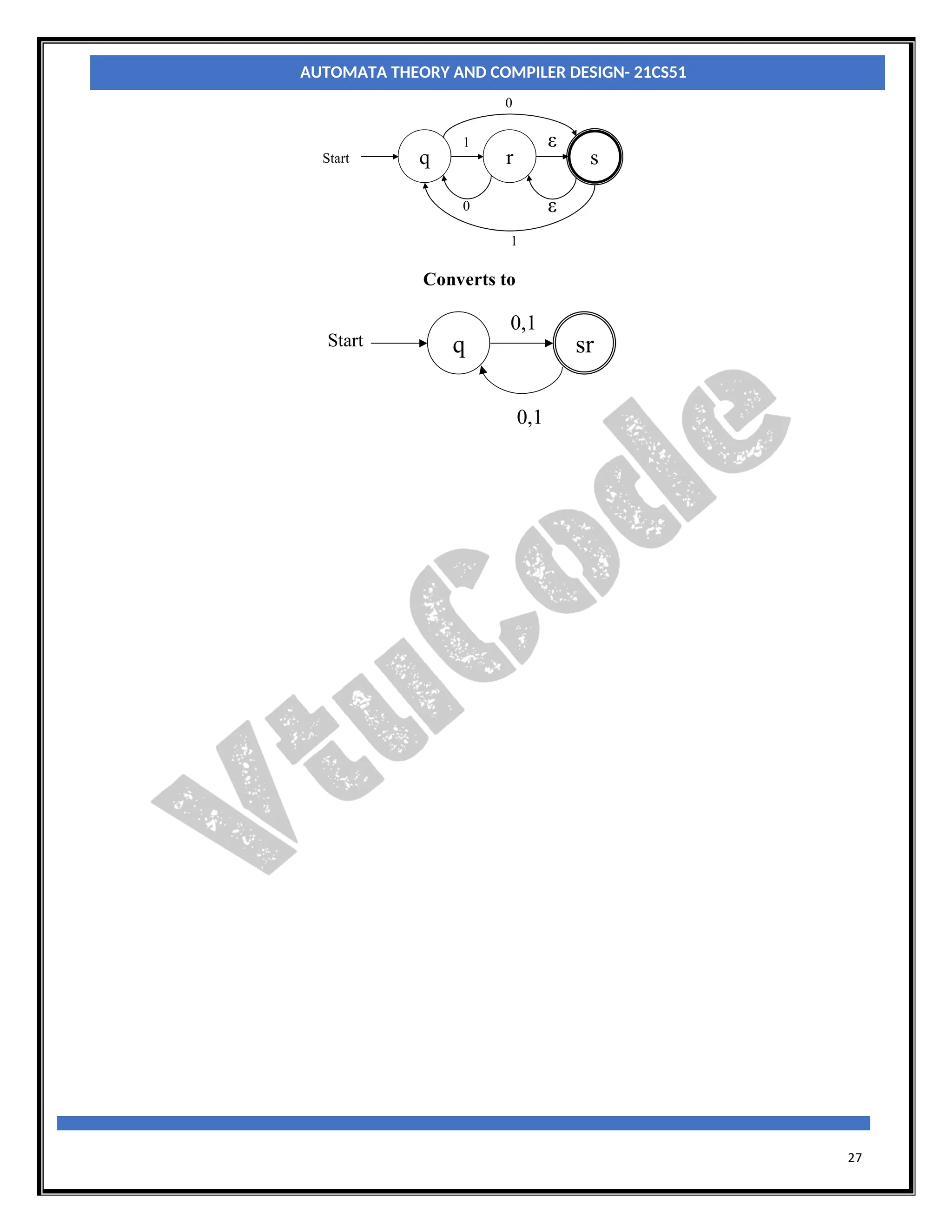
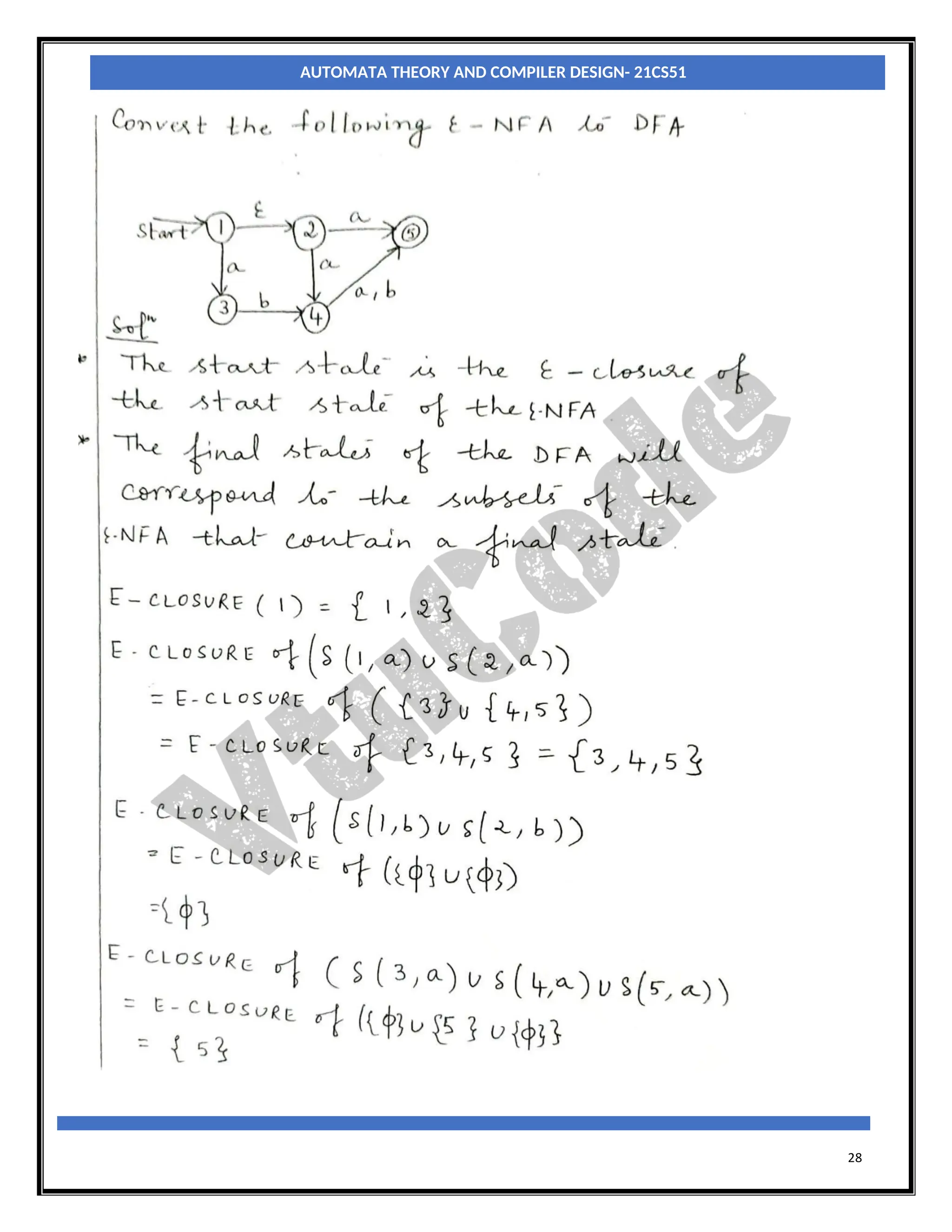
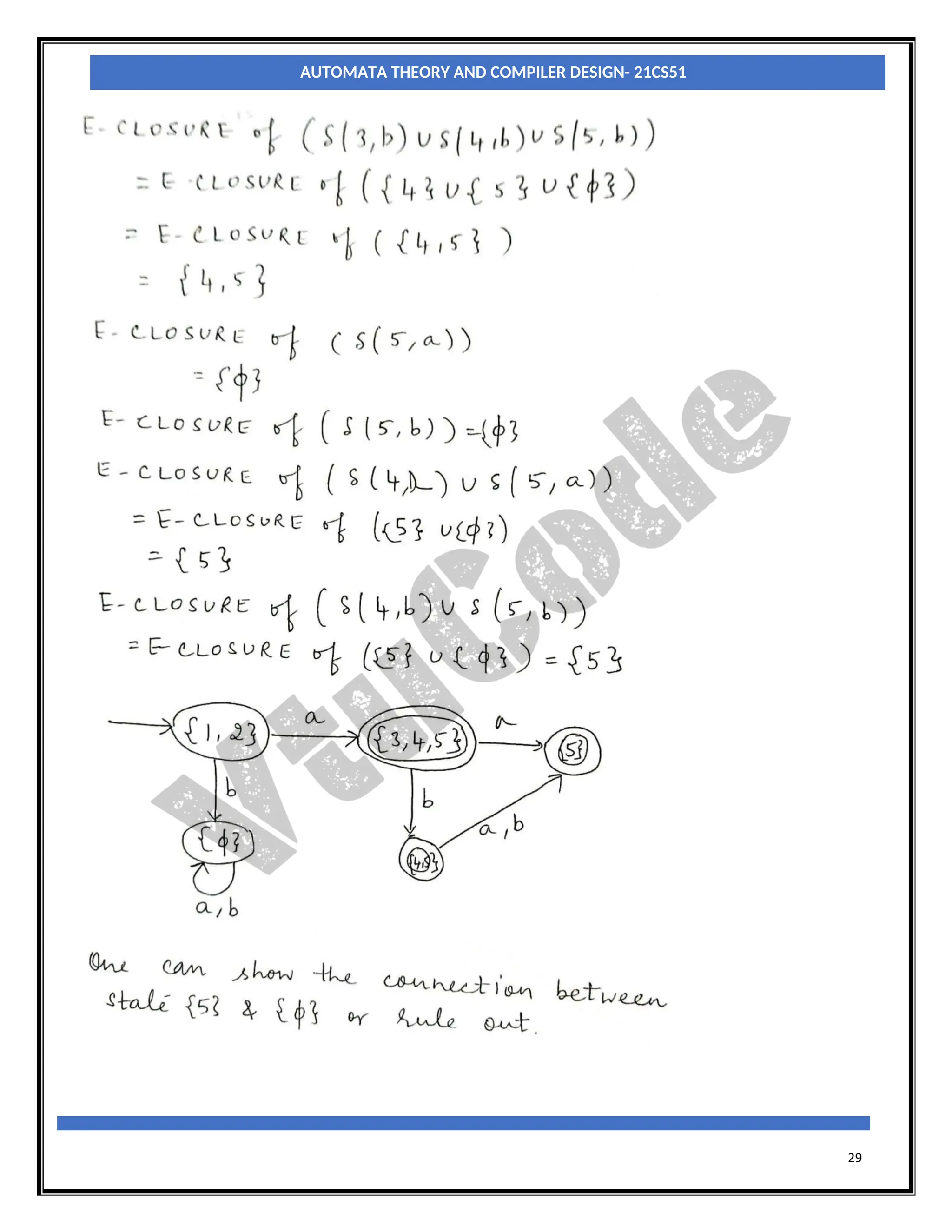
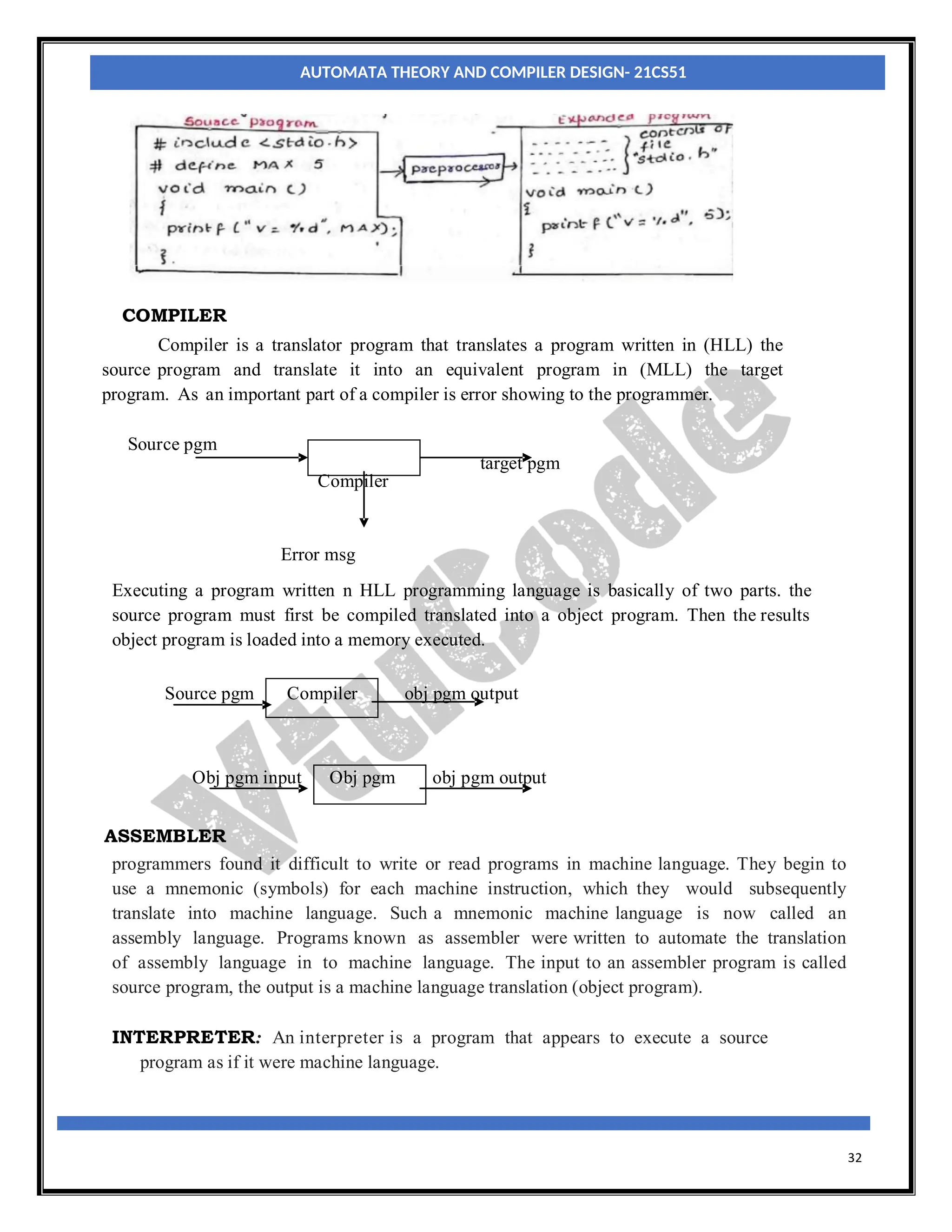
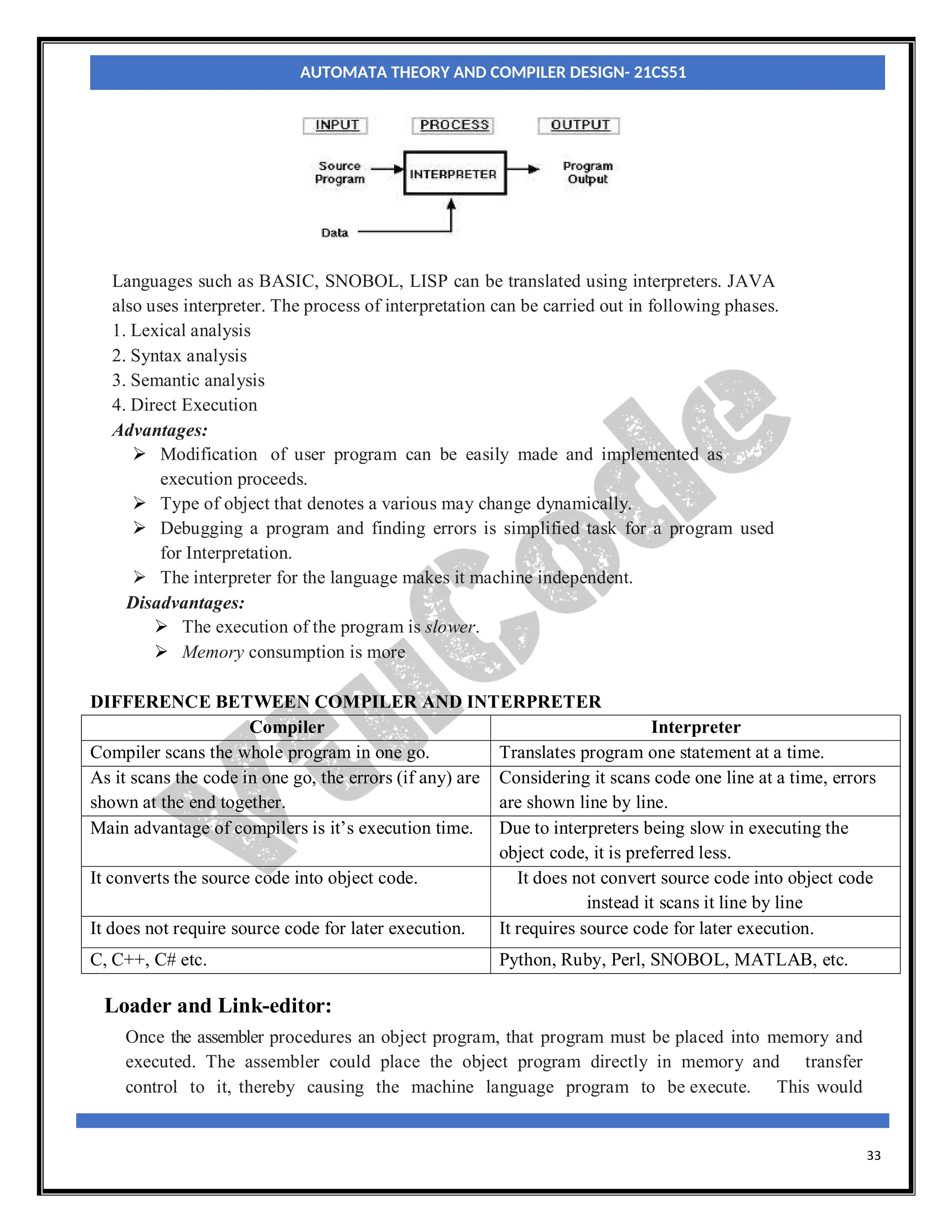
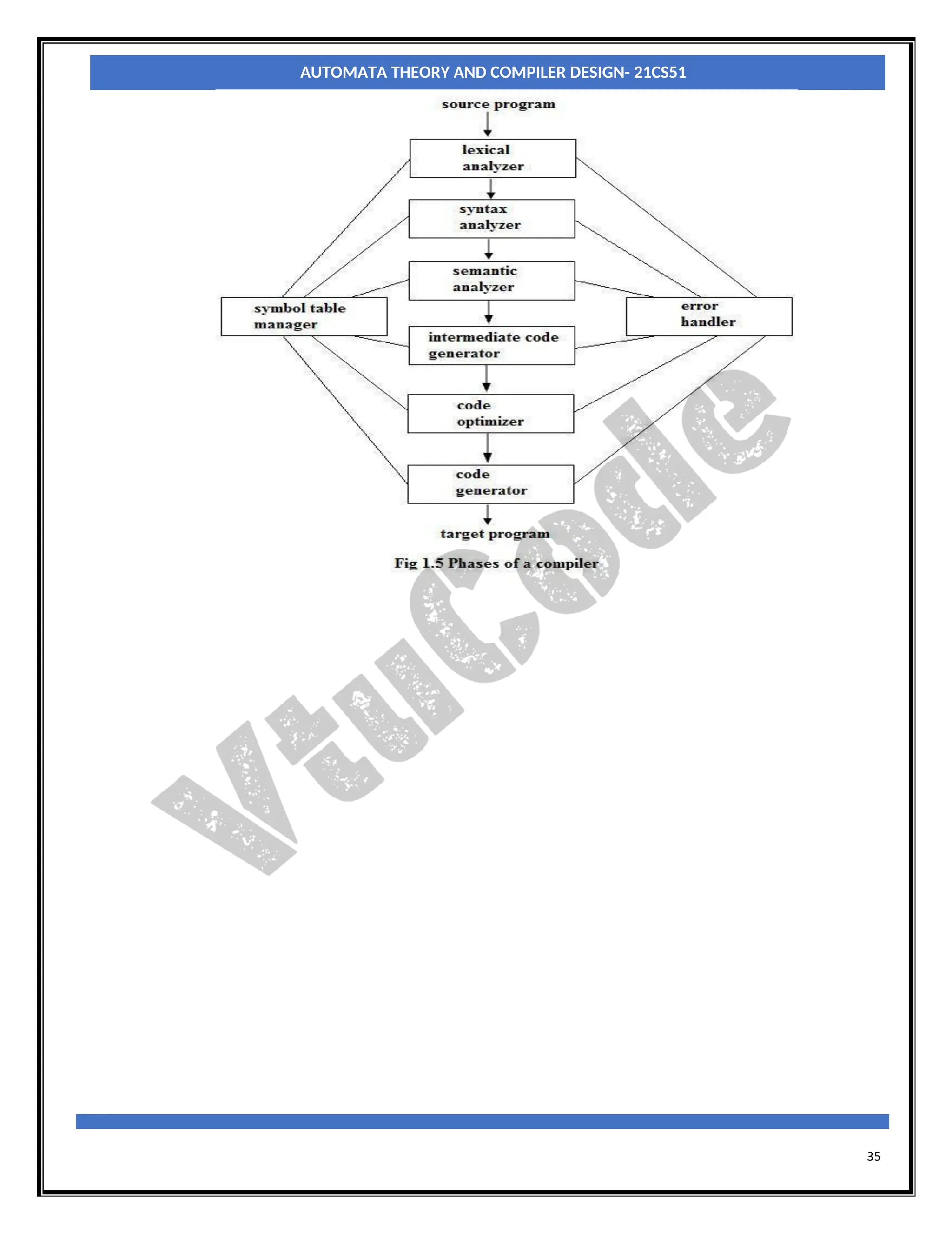
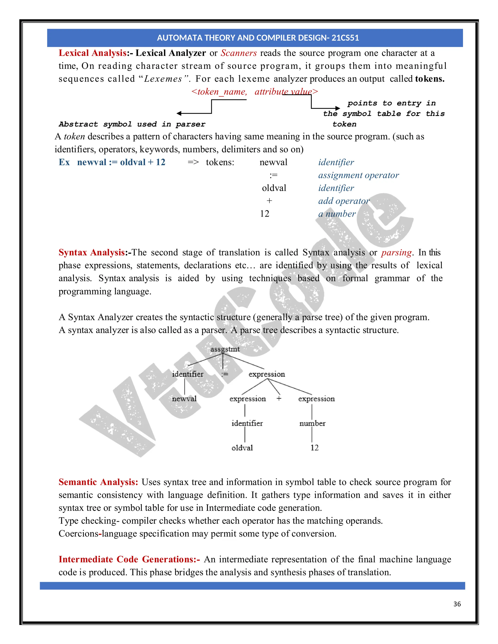
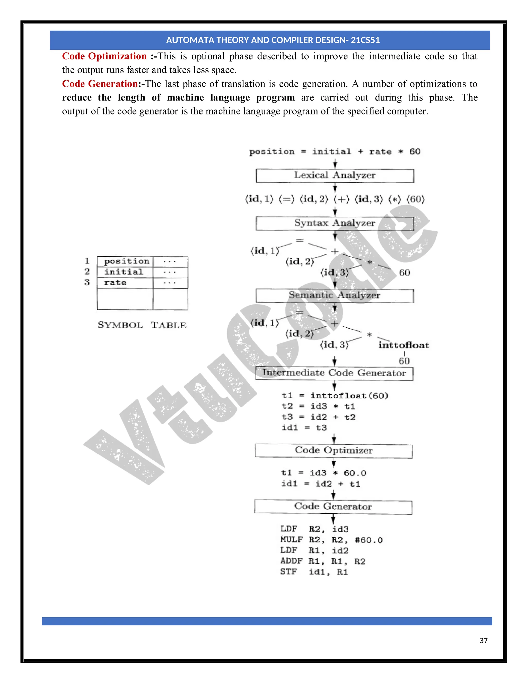
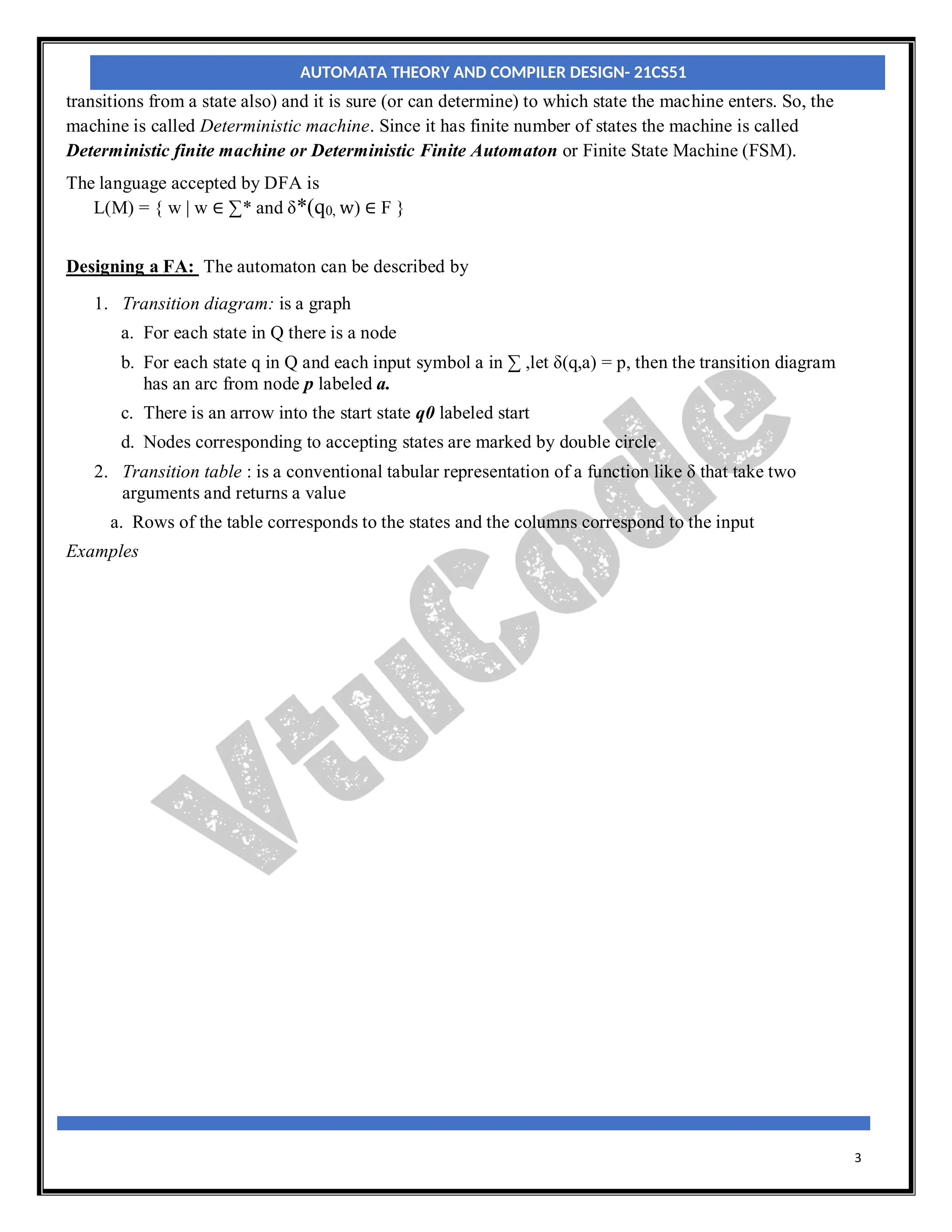
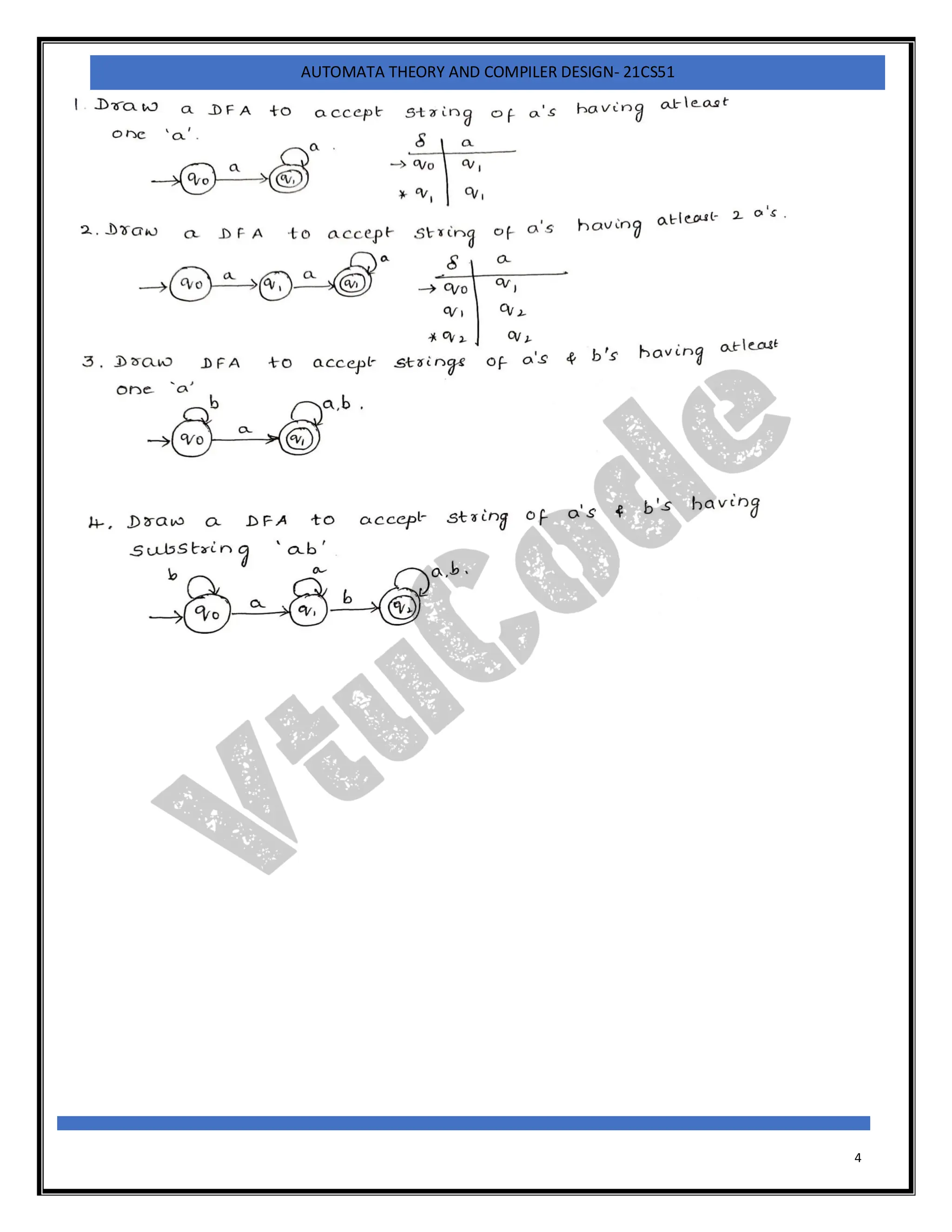
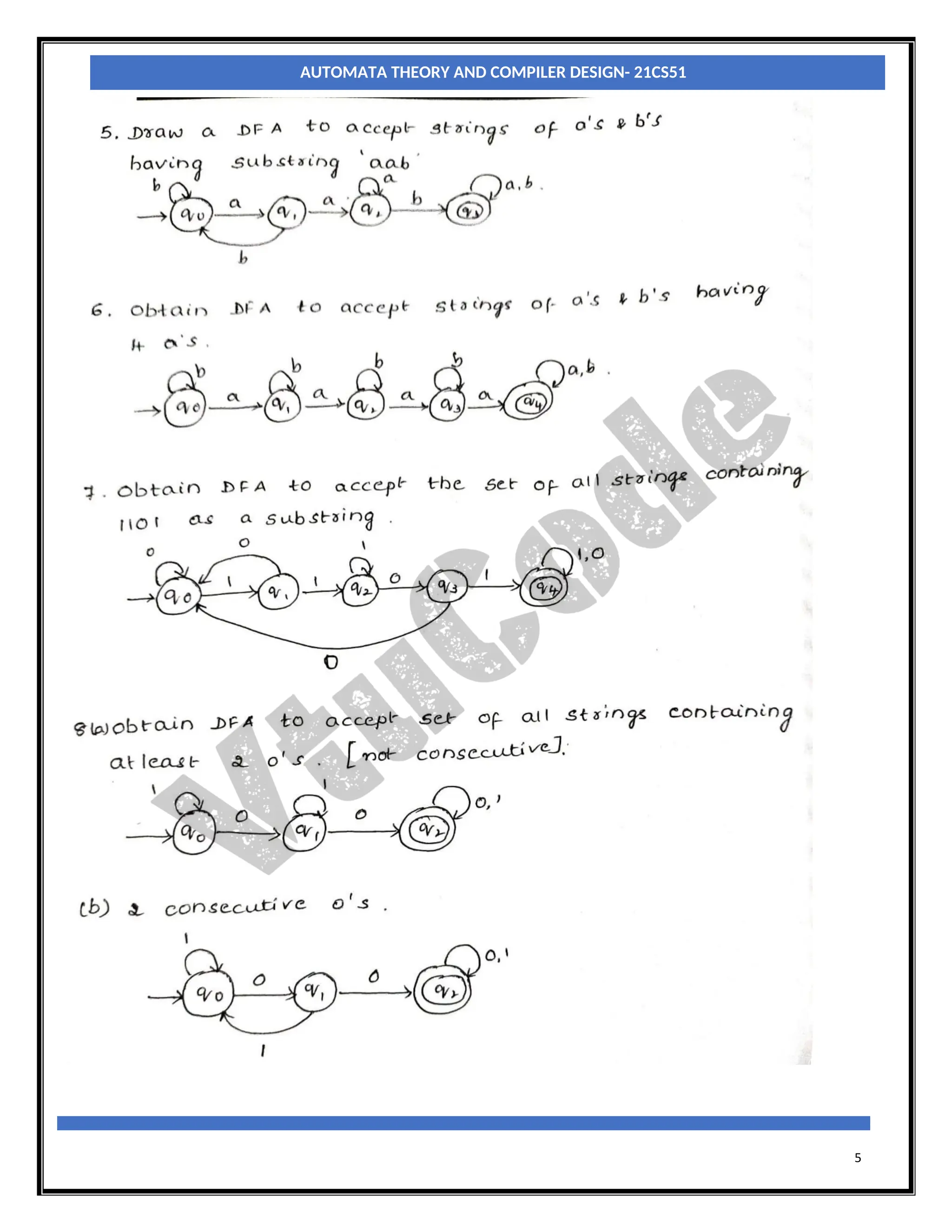
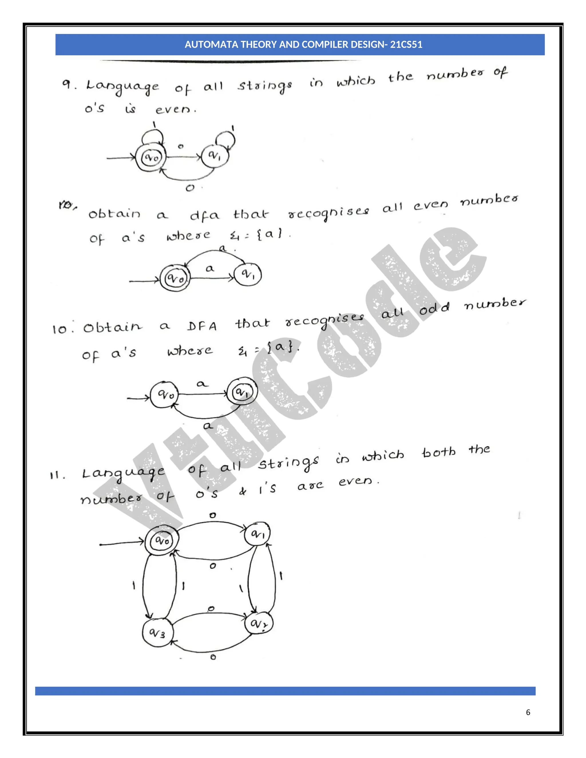
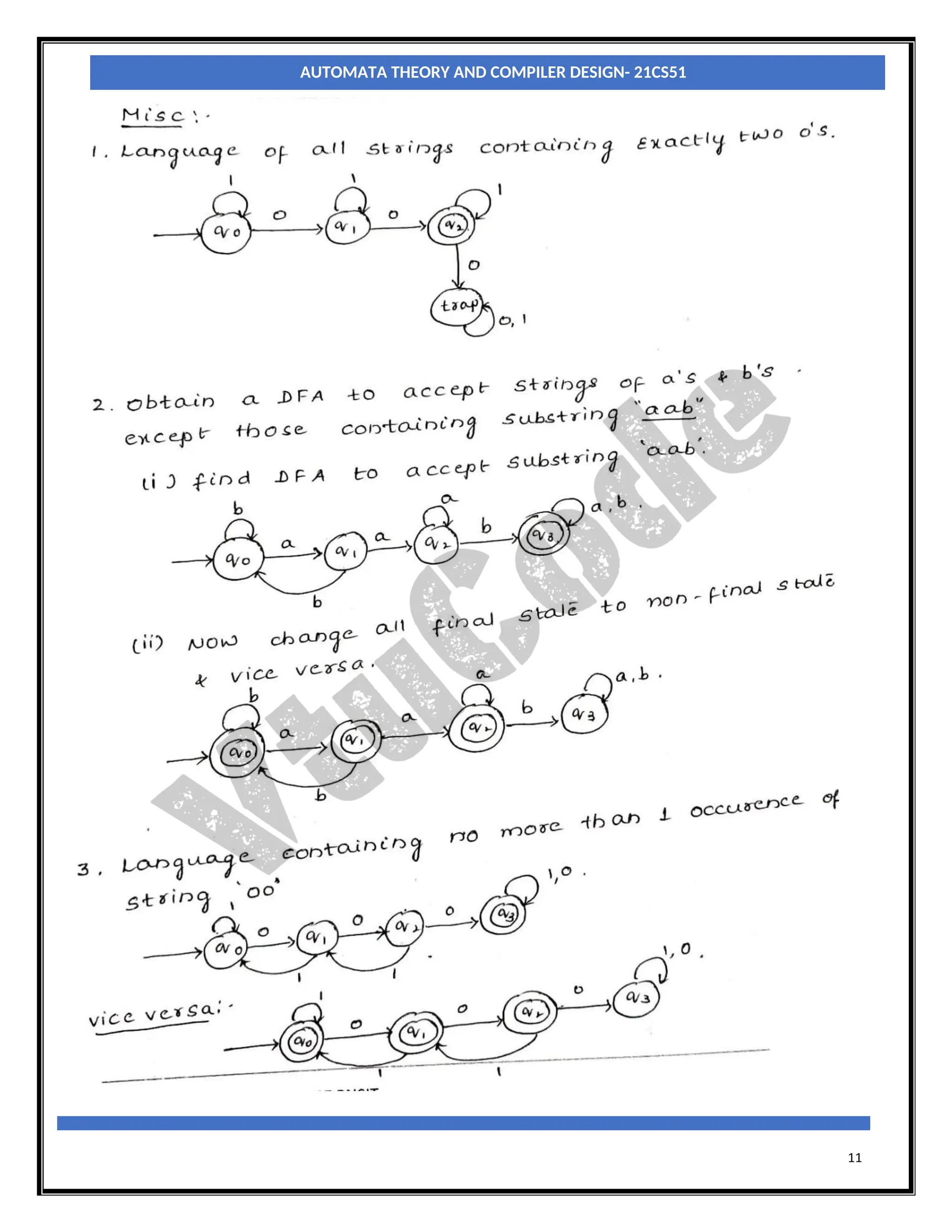
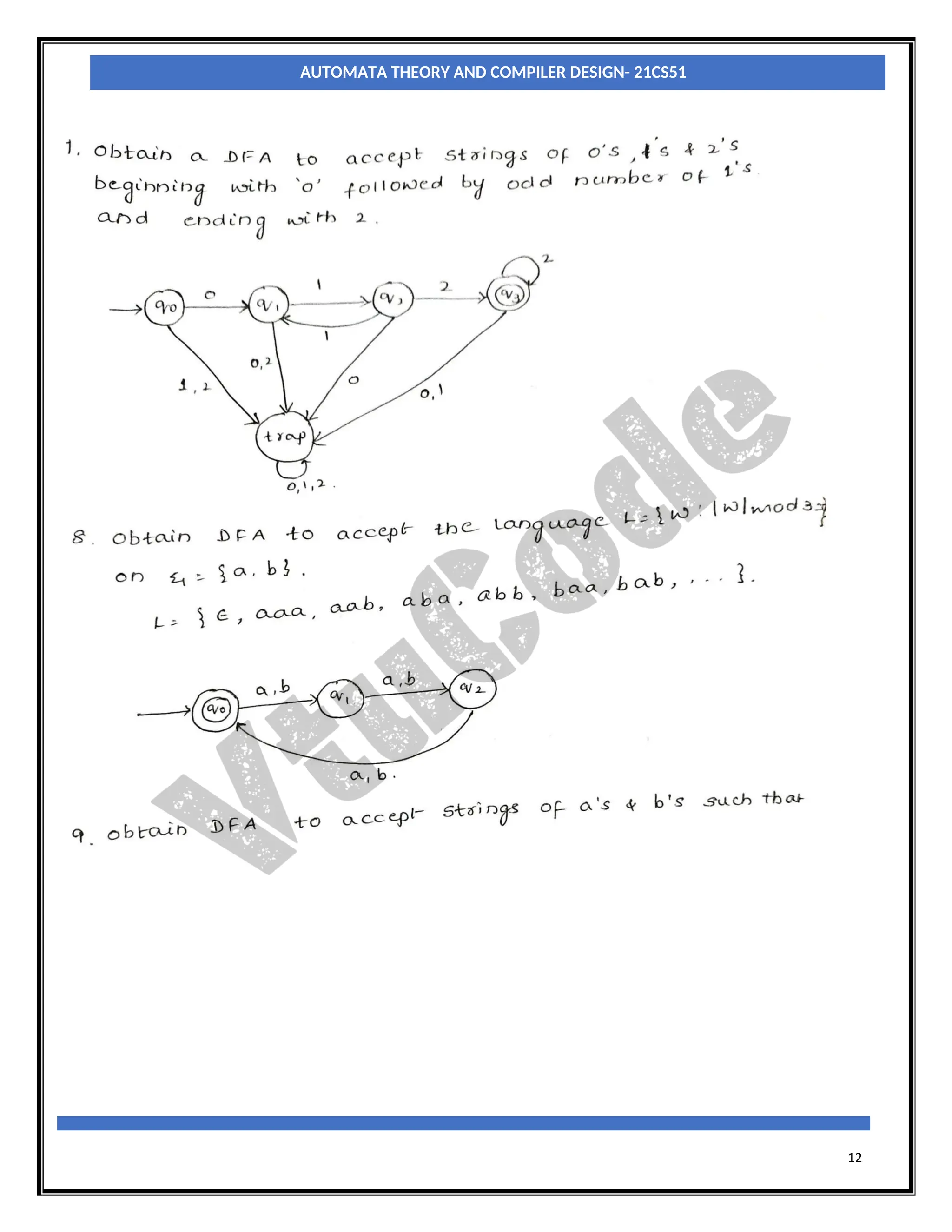
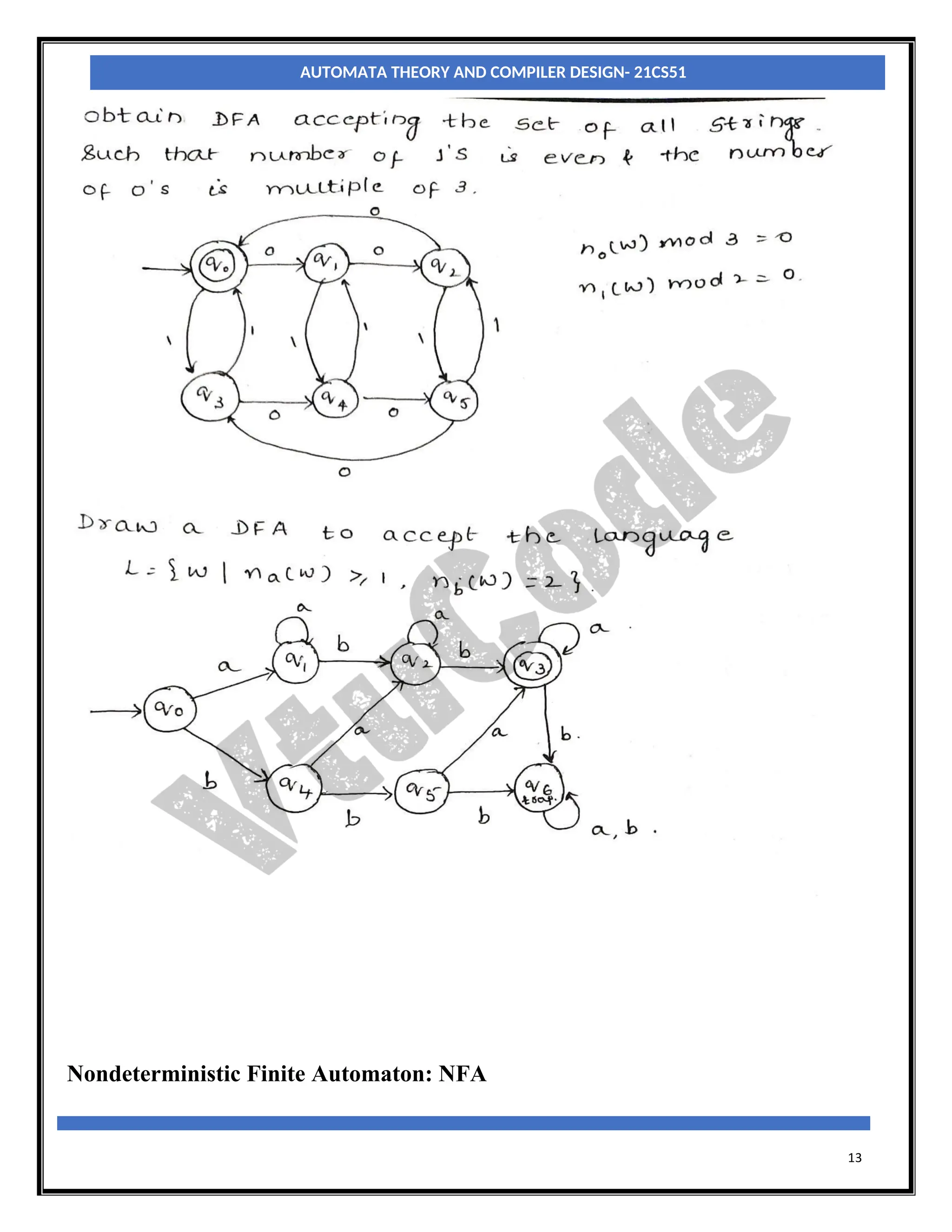
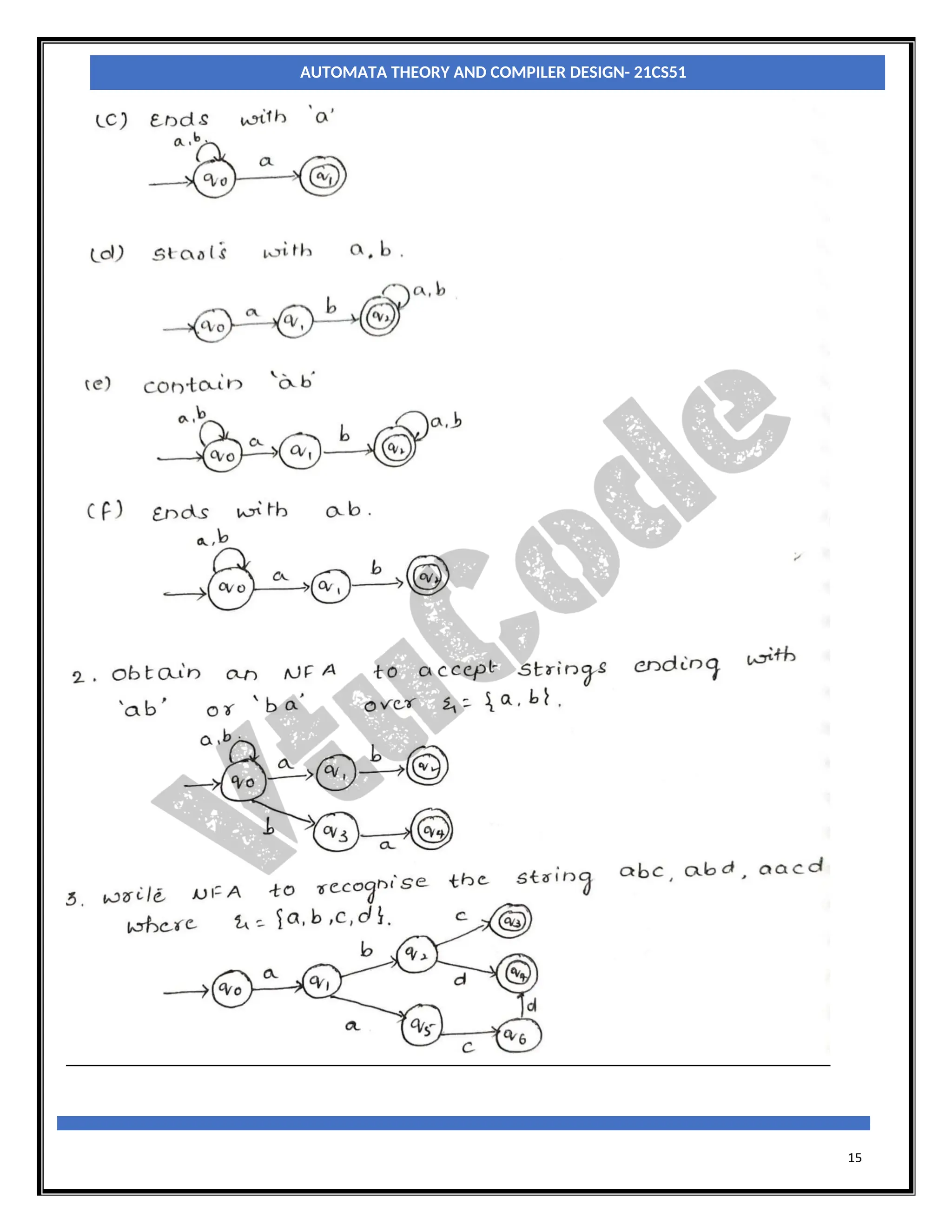
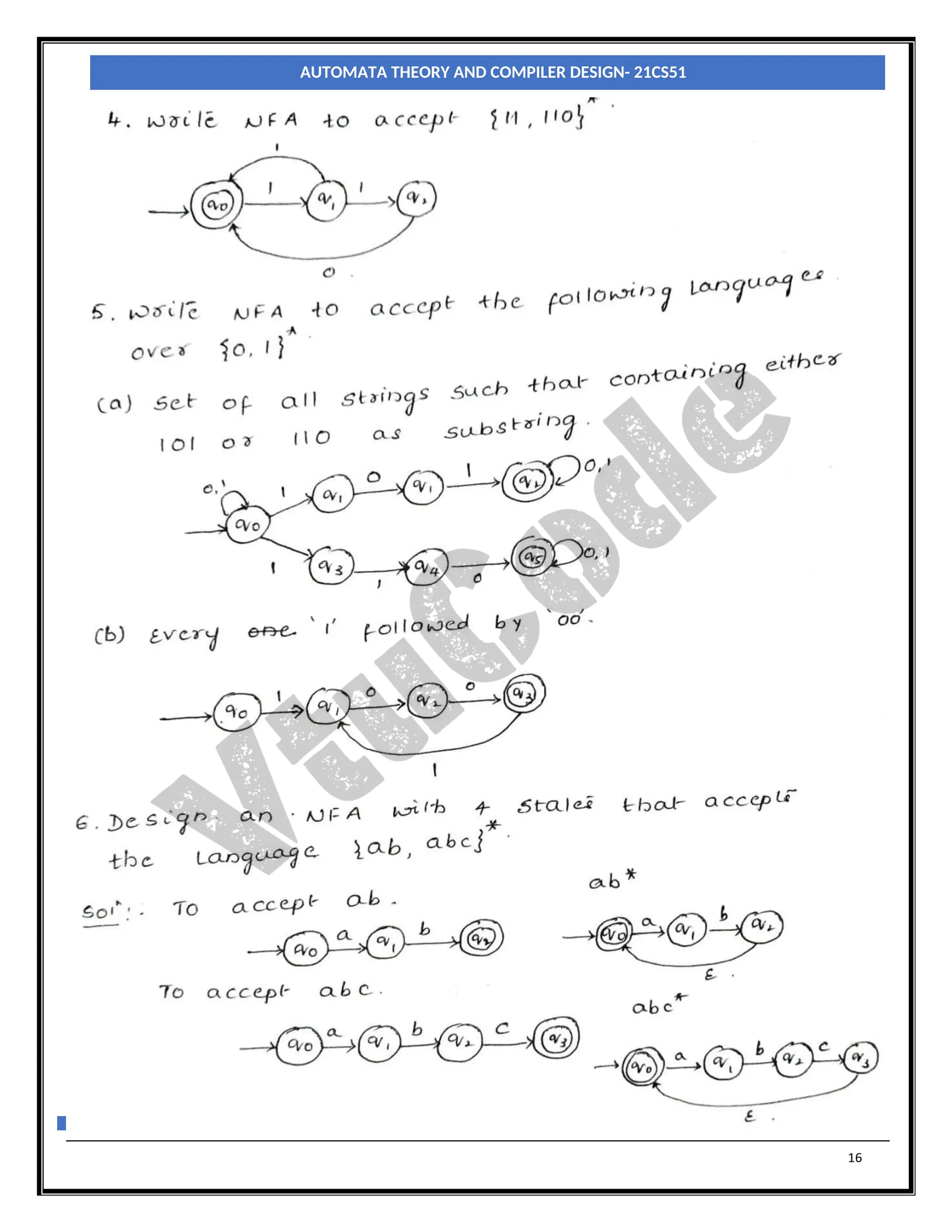
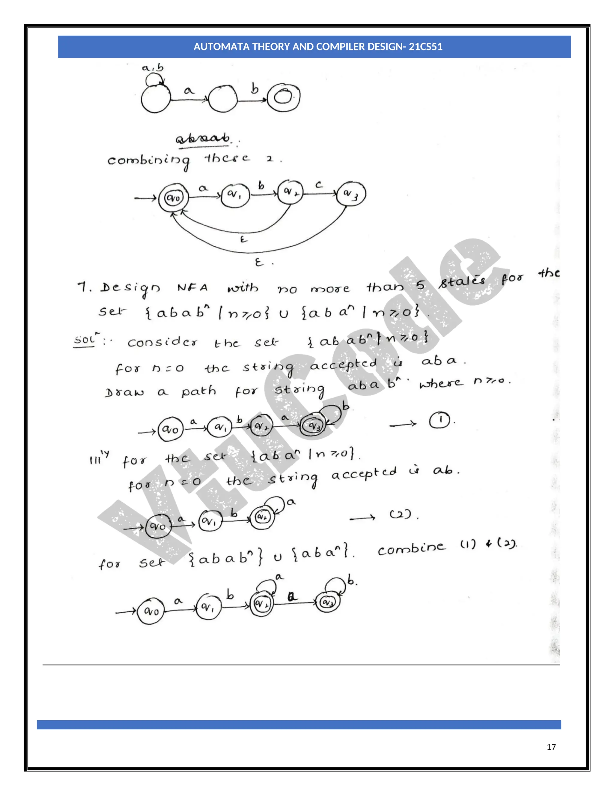
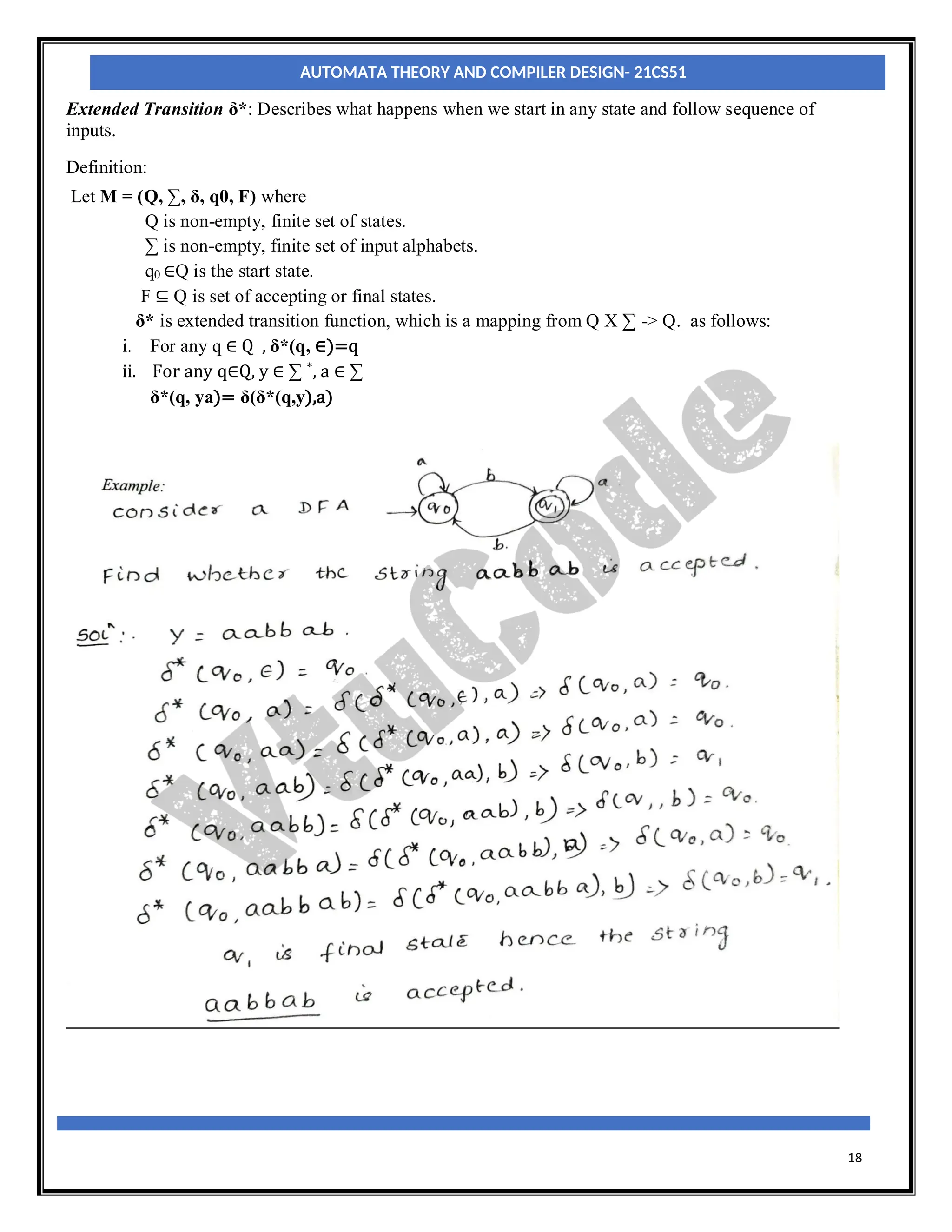
The document provides an introduction to automata theory and finite automata. It discusses key concepts such as alphabets, strings, languages, deterministic finite automata (DFAs), nondeterministic finite automata (NFAs), epsilon-NFAs, and the process of converting an NFA to a DFA using subset construction. The summary is:
[1] Automata theory studies abstract computing devices called automata and finite automata are a useful model for hardware and software. [2] Finite automata can be deterministic (DFAs) or nondeterministic (NFAs) and accept regular languages. [3] NFAs allow ambiguous transitions while DFAs have a single unambiguous transition for each state


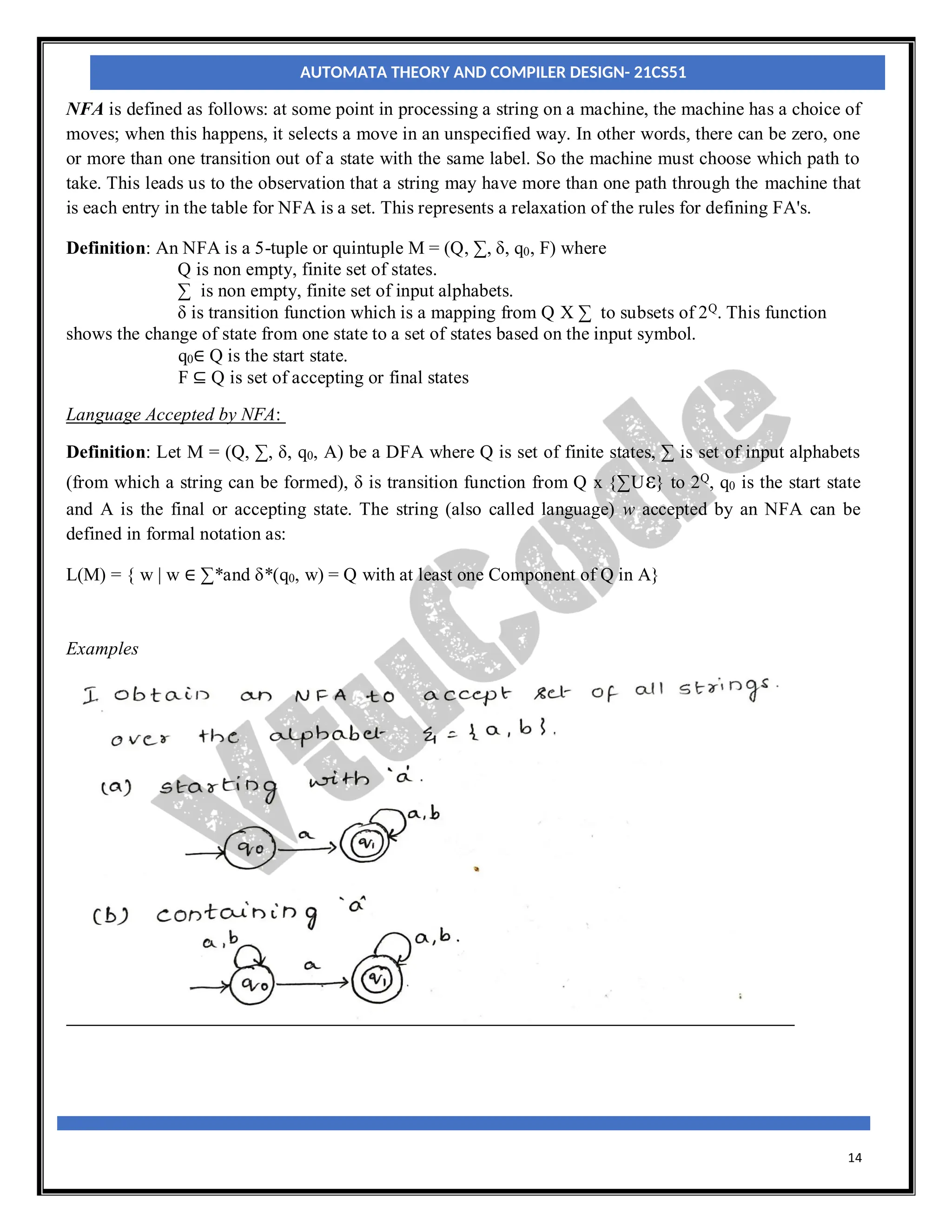
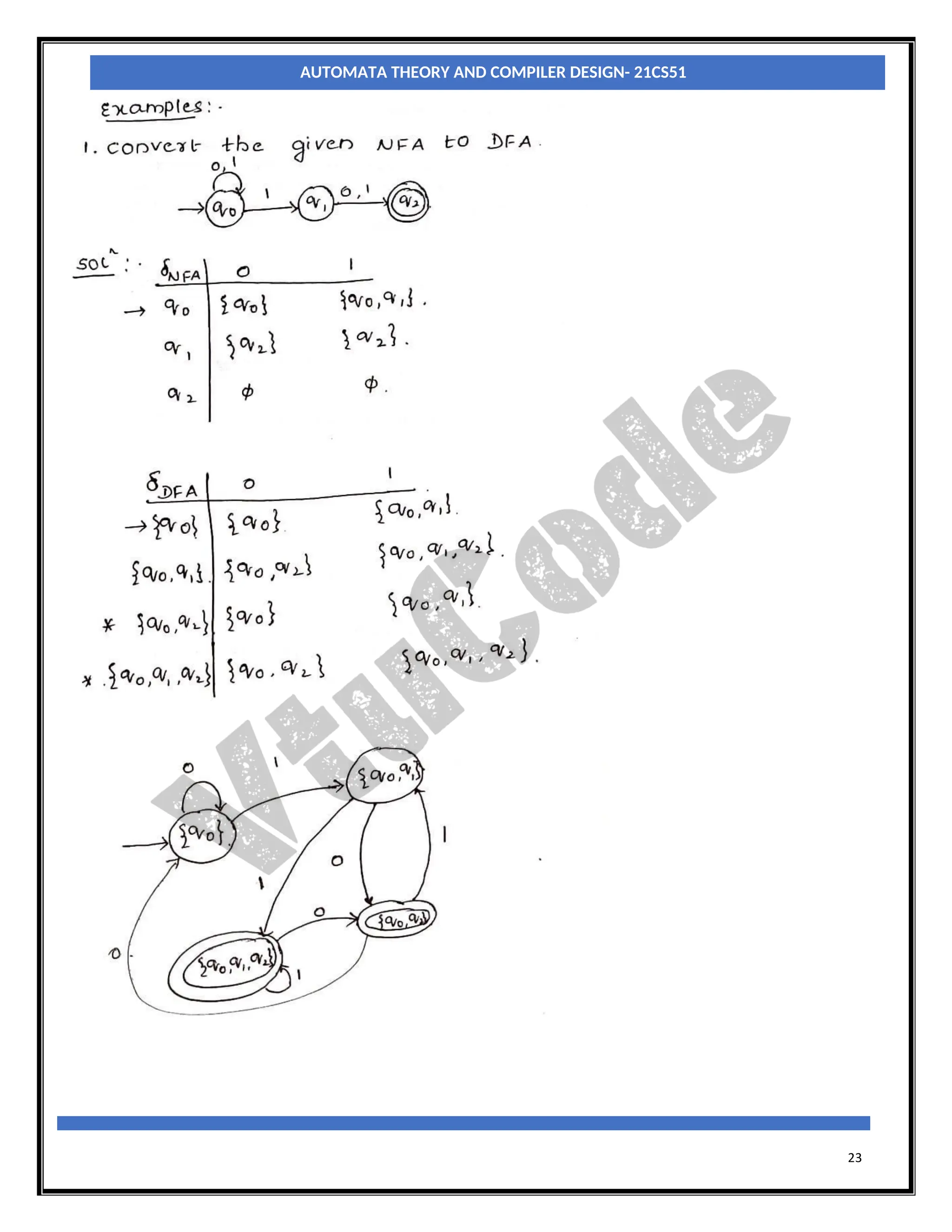
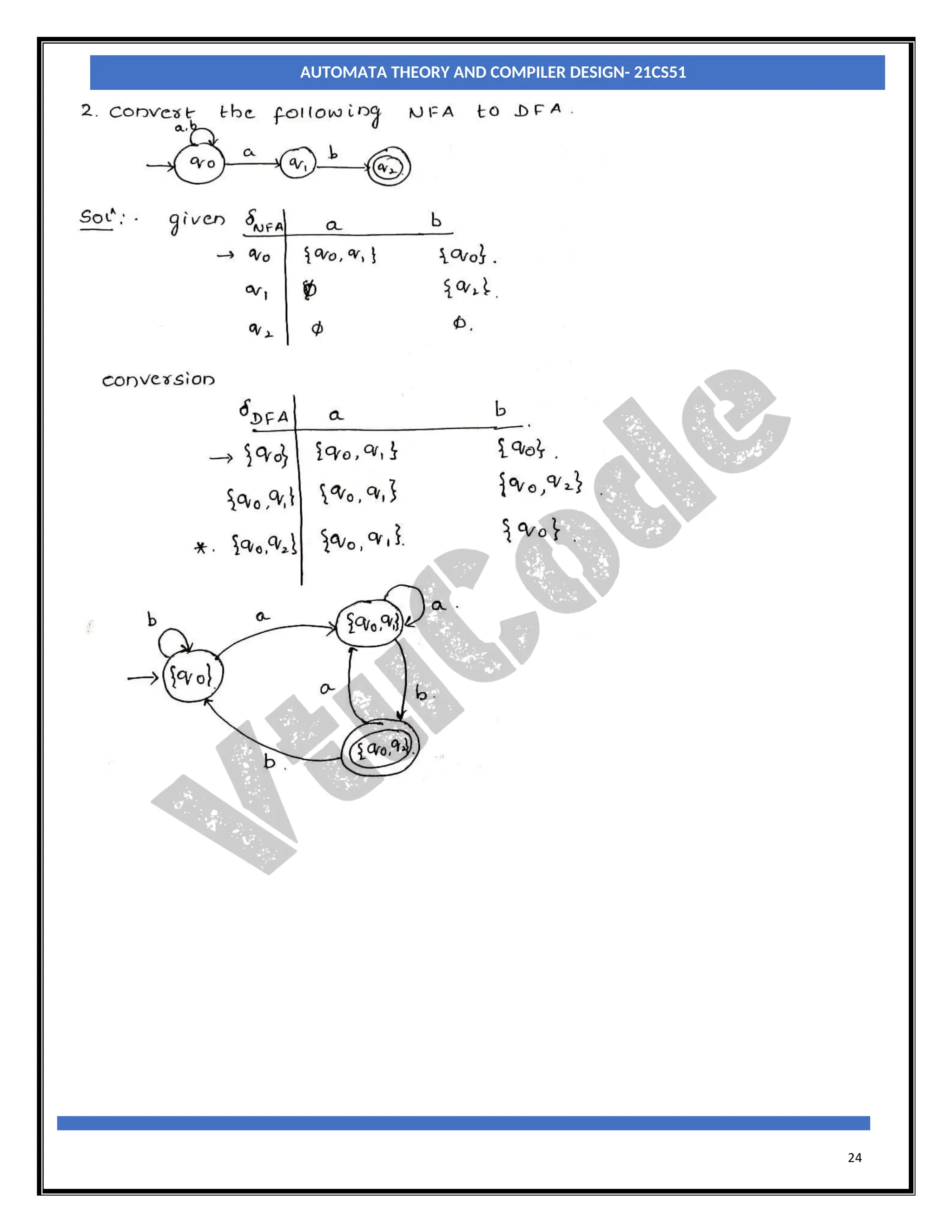
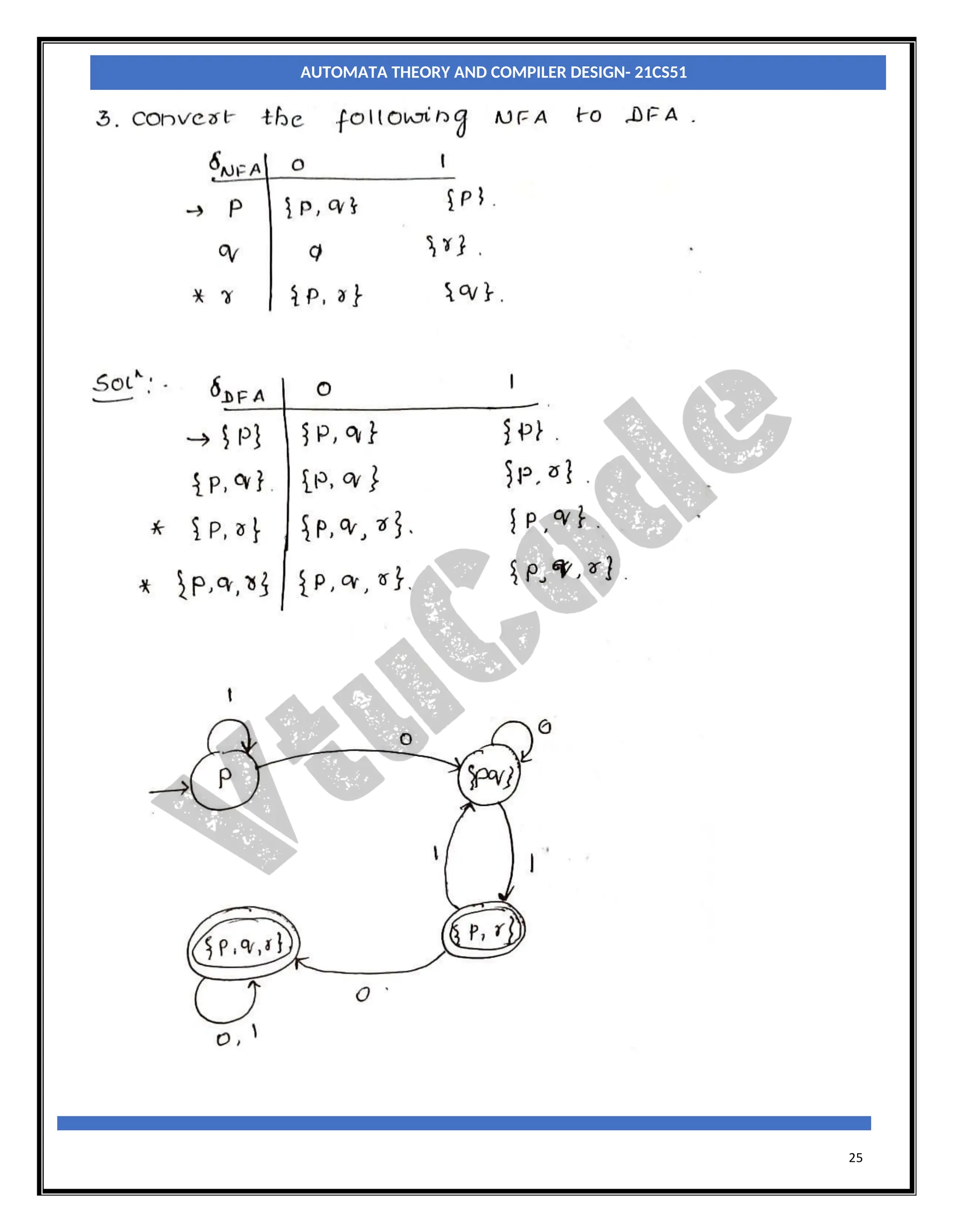
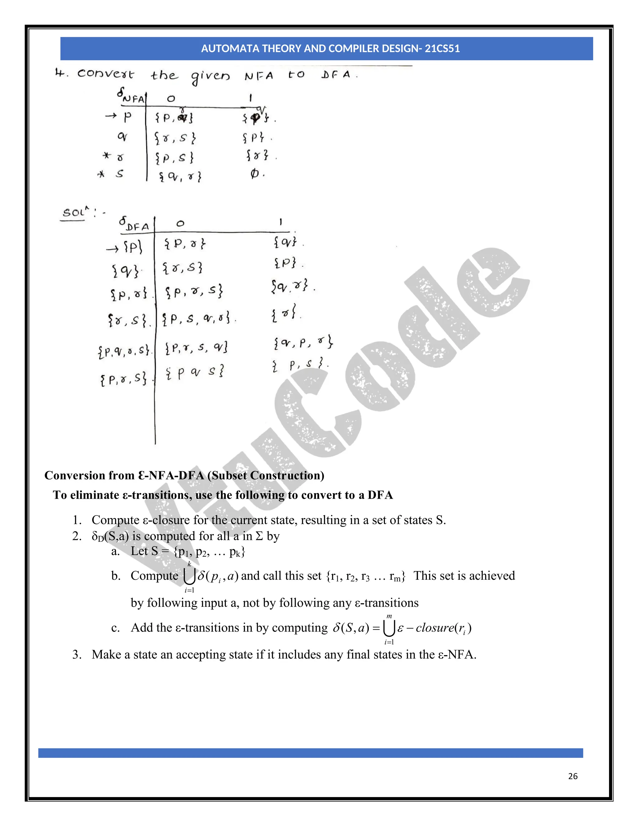
![22
With an NFA, at any point in a scanning of the input string we may be faced with a choice of any number
of paths to be followed to reach a final state. With a DFA there is never a choice of paths. So, when we
construct a DFA which accepts the same language as a particular NFA, the conversion process effectively
involves merging all possible states which can be reached on a particular input character, from a particular
state, into a single, composite, state which represents all those paths.
Let MN = (QN, ∑, δN, q0, FN) be an NFA and accepts the language L(MN). There should be an equivalent
DFA MD = (QD, ∑D, δD, q0, FD) such that L(MD) = L(MN). The procedure to convert an NFA to its
equivalent DFA is shown below
Step1: The start state of NFA MN is the start state of DFA MD. So, add q0(which is the start state of NFA)
to QD and find the transitions from this state.
Step2: For each state [qi, qj,….qk] in QD, the transitions for each input symbol in ∑ can be obtained as
shown below:
δD([qi, qj,….qk], a) = δN(qi, a) U δN(qj, a) U ……δN(qk, a)
a =[ql,qm,….qn]say.
Add the state [ql, qm,….qn] to QD, if it is not already in QD.
Add the transition from [qi, qj,….qk] to [ql, qm,….qn] on the input symbol α iff the state [ql,
qm,….qn] is added to QD in the previous step.
Step3: The state [qa, qb,….qc] ∈ QD is the final state, if at least one of the state in qa, qb, ….. qc∈ AN i.e., at
least one of the component in [qa, qb,….qc] should be the final state of NFA.
AUTOMATA THEORY AND COMPILER DESIGN- 21CS51](https://image.slidesharecdn.com/vtucode-240205145809-819fe16c/75/vtucode-in-module-1-21CS51-5th-semester-1-pdf-22-2048.jpg)