SlideShare a Scribd company logo
1 of 1733
Download to read offline
1-1
Chapter 1
INTRODUCTION AND BASIC CONCEPTS
Thermodynamics
1-1C Classical thermodynamics is based on experimental observations whereas statistical thermodynamics
is based on the average behavior of large groups of particles.
1-2C On a downhill road the potential energy of the bicyclist is being converted to kinetic energy, and
thus the bicyclist picks up speed. There is no creation of energy, and thus no violation of the conservation
of energy principle.
1-3C There is no truth to his claim. It violates the second law of thermodynamics.
Mass, Force, and Units
1-4C Pound-mass lbm is the mass unit in English system whereas pound-force lbf is the force unit. One
pound-force is the force required to accelerate a mass of 32.174 lbm by 1 ft/s2
. In other words, the weight
of a 1-lbm mass at sea level is 1 lbf.
1-5C Kg-mass is the mass unit in the SI system whereas kg-force is a force unit. 1-kg-force is the force
required to accelerate a 1-kg mass by 9.807 m/s2
. In other words, the weight of 1-kg mass at sea level is 1
kg-force.
1-6C There is no acceleration, thus the net force is zero in both cases.
1-7 A plastic tank is filled with water. The weight of the combined system is to be determined.
Assumptions The density of water is constant throughout.
Properties The density of water is given to be ρ = 1000 kg/m3
.
Analysis The mass of the water in the tank and the total mass are mtank = 3 kg
V =0.2 m
3
H2O
mw =ρV =(1000 kg/m3
)(0.2 m3
) = 200 kg
mtotal = mw + mtank = 200 + 3 = 203 kg
Thus,
N
1991
m/s
kg
1
N
1
)
m/s
kg)(9.81
(203 2
2
=








⋅
=
= mg
W
1-2
1-8 The interior dimensions of a room are given. The mass and weight of the air in the room are to be
determined.
Assumptions The density of air is constant throughout the room.
Properties The density of air is given to be ρ = 1.16 kg/m3
.
ROOM
AIR
6X6X8 m3
Analysis The mass of the air in the room is
kg
334.1
=
×
×
=
= )
m
8
6
)(6
kg/m
(1.16 3
3
V
ρ
m
Thus,
N
3277
=








⋅
=
= 2
2
m/s
kg
1
N
1
)
m/s
kg)(9.81
(334.1
mg
W
1-9 The variation of gravitational acceleration above the sea level is given as a function of altitude. The
height at which the weight of a body will decrease by 1% is to be determined.
0
z
Analysis The weight of a body at the elevation z can be expressed as
W mg m z
= = − × −
( . . )
9 807 332 10 6
In our case,
W W mg m
s s
= = =
099 0 99 0 99 9807
. . . ( )( . )
Substituting,
m
29,539
=
→

×
−
= −
z
z)
10
32
.
3
81
.
9
(
)
81
.
9
(
99
.
0 6
Sea level
1-10E An astronaut took his scales with him to space. It is to be determined how much he will weigh on
the spring and beam scales in space.
Analysis (a) A spring scale measures weight, which is the local gravitational force applied on a body:
lbf
25.5
=








⋅
=
= 2
2
ft/s
lbm
32.2
lbf
1
)
ft/s
lbm)(5.48
(150
mg
W
(b) A beam scale compares masses and thus is not affected by the variations in gravitational acceleration.
The beam scale will read what it reads on earth,
W = 150 lbf
1-11 The acceleration of an aircraft is given in g’s. The net upward force acting on a man in the aircraft is
to be determined.
Analysis From the Newton's second law, the force applied is
N
5297
=








⋅
×
=
=
= 2
2
m/s
kg
1
N
1
)
m/s
9.81
kg)(6
(90
)
g
6
(
m
ma
F
1-3
1-12 [Also solved by EES on enclosed CD] A rock is thrown upward with a specified force. The
acceleration of the rock is to be determined.
Analysis The weight of the rock is
N
48.95
=








⋅
=
= 2
2
m/s
kg
1
N
1
)
m/s
kg)(9.79
(5
mg
W
Then the net force that acts on the rock is
N
101.05
48.95
150
down
up
net =
−
=
−
= F
F
F
From the Newton's second law, the acceleration of the rock becomes Stone
2
m/s
20.2
=







 ⋅
=
=
N
1
m/s
kg
1
kg
5
N
101.05 2
m
F
a
1-13 EES Problem 1-12 is reconsidered. The entire EES solution is to be printed out, including the
numerical results with proper units.
Analysis The problem is solved using EES, and the solution is given below.
W=m*g"[N]"
m=5"[kg]"
g=9.79"[m/s^2]"
"The force balance on the rock yields the net force acting on the rock as"
F_net = F_up - F_down"[N]"
F_up=150"[N]"
F_down=W"[N]"
"The acceleration of the rock is determined from Newton's second law."
F_net=a*m
"To Run the program, press F2 or click on the calculator icon from the Calculate menu"
SOLUTION
a=20.21 [m/s^2]
F_down=48.95 [N]
F_net=101.1 [N]
F_up=150 [N]
g=9.79 [m/s^2]
m=5 [kg]
W=48.95 [N]
1-4
1-14 Gravitational acceleration g and thus the weight of bodies decreases with increasing elevation. The
percent reduction in the weight of an airplane cruising at 13,000 m is to be determined.
Properties The gravitational acceleration g is given to be 9.807 m/s2
at sea level and 9.767 m/s2
at an
altitude of 13,000 m.
Analysis Weight is proportional to the gravitational acceleration g, and thus the
percent reduction in weight is equivalent to the percent reduction in the
gravitational acceleration, which is determined from
0.41%
=
×
−
=
×
∆
=
= 100
807
.
9
767
.
9
807
.
9
100
in
%Reduction
in weight
%Reduction
g
g
g
Therefore, the airplane and the people in it will weight
0.41% less at 13,000 m altitude.
Discussion Note that the weight loss at cruising altitudes is negligible.
Systems, Properties, State, and Processes
1-15C The radiator should be analyzed as an open system since mass is crossing the boundaries of the
system.
1-16C A can of soft drink should be analyzed as a closed system since no mass is crossing the boundaries
of the system.
1-17C Intensive properties do not depend on the size (extent) of the system but extensive properties do.
1-18C For a system to be in thermodynamic equilibrium, the temperature has to be the same throughout
but the pressure does not. However, there should be no unbalanced pressure forces present. The increasing
pressure with depth in a fluid, for example, should be balanced by increasing weight.
1-19C A process during which a system remains almost in equilibrium at all times is called a quasi-
equilibrium process. Many engineering processes can be approximated as being quasi-equilibrium. The
work output of a device is maximum and the work input to a device is minimum when quasi-equilibrium
processes are used instead of nonquasi-equilibrium processes.
1-20C A process during which the temperature remains constant is called isothermal; a process during
which the pressure remains constant is called isobaric; and a process during which the volume remains
constant is called isochoric.
1-21C The state of a simple compressible system is completely specified by two independent, intensive
properties.
1-22C Yes, because temperature and pressure are two independent properties and the air in an isolated
room is a simple compressible system.
1-23C A process is said to be steady-flow if it involves no changes with time anywhere within the system
or at the system boundaries.
1-24C The specific gravity, or relative density, and is defined as the ratio of the density of a substance to
the density of some standard substance at a specified temperature (usually water at 4°C, for which ρH2O =
1000 kg/m3
). That is, SG H2O
/ ρ
ρ
= . When specific gravity is known, density is determined from
H2O
SG ρ
ρ ×
= .
1-5
1-25 EES The variation of density of atmospheric air with elevation is given in tabular form. A relation for
the variation of density with elevation is to be obtained, the density at 7 km elevation is to be calculated,
and the mass of the atmosphere using the correlation is to be estimated.
Assumptions 1 Atmospheric air behaves as an ideal gas. 2 The earth is perfectly sphere with a radius of
6377 km, and the thickness of the atmosphere is 25 km.
Properties The density data are given in tabular form as
r, km z, km ρ, kg/m3
6377 0 1.225
6378 1 1.112
6379 2 1.007
6380 3 0.9093
6381 4 0.8194
6382 5 0.7364
6383 6 0.6601
6385 8 0.5258
6387 10 0.4135
6392 15 0.1948
6397 20 0.08891
6402 25 0.04008
0 5 10 15 20 25
0
0.2
0.4
0.6
0.8
1
1.2
1.4
z, km
ρ
,
kg/m
3
Analysis Using EES, (1) Define a trivial function rho= a+z in equation window, (2) select new parametric
table from Tables, and type the data in a two-column table, (3) select Plot and plot the data, and (4) select
plot and click on “curve fit” to get curve fit window. Then specify 2nd
order polynomial and enter/edit
equation. The results are:
ρ(z) = a + bz + cz2
= 1.20252 – 0.101674z + 0.0022375z2
for the unit of kg/m3
,
(or, ρ(z) = (1.20252 – 0.101674z + 0.0022375z2
)×109
for the unit of kg/km3
)
where z is the vertical distance from the earth surface at sea level. At z = 7 km, the equation would give ρ =
0.60 kg/m3
.
(b) The mass of atmosphere can be evaluated by integration to be
[ ]
5
/
4
/
)
2
(
3
/
)
2
(
2
/
)
2
(
4
)
2
)(
(
4
)
(
4
)
(
5
4
0
3
2
0
0
2
0
0
2
0
2
0
2
0
2
0
2
0
2
0
ch
h
cr
b
h
cr
br
a
h
br
a
r
h
ar
dz
z
z
r
r
cz
bz
a
dz
z
r
cz
bz
a
dV
m
h
z
h
z
V
+
+
+
+
+
+
+
+
=
+
+
+
+
=
+
+
+
=
= ∫
∫
∫ =
=
π
π
π
ρ
where r0 = 6377 km is the radius of the earth, h = 25 km is the thickness of the atmosphere, and a =
1.20252, b = -0.101674, and c = 0.0022375 are the constants in the density function. Substituting and
multiplying by the factor 109
for the density unity kg/km3
, the mass of the atmosphere is determined to be
m = 5.092×10¹⁸
kg
Discussion Performing the analysis with excel would yield exactly the same results.
EES Solution for final result:
a=1.2025166
b=-0.10167
c=0.0022375
r=6377
h=25
m=4*pi*(a*r^2*h+r*(2*a+b*r)*h^2/2+(a+2*b*r+c*r^2)*h^3/3+(b+2*c*r)*h^4/4+c*h^5/5)*1E+9
1-6
Temperature
1-26C The zeroth law of thermodynamics states that two bodies are in thermal equilibrium if both have the
same temperature reading, even if they are not in contact.
1-27C They are celsius(°C) and kelvin (K) in the SI, and fahrenheit (°F) and rankine (R) in the English
system.
1-28C Probably, but not necessarily. The operation of these two thermometers is based on the thermal
expansion of a fluid. If the thermal expansion coefficients of both fluids vary linearly with temperature,
then both fluids will expand at the same rate with temperature, and both thermometers will always give
identical readings. Otherwise, the two readings may deviate.
1-29 A temperature is given in °C. It is to be expressed in K.
Analysis The Kelvin scale is related to Celsius scale by
T(K] = T(°C) + 273
Thus, T(K] = 37°C + 273 = 310 K
1-30E A temperature is given in °C. It is to be expressed in °F, K, and R.
Analysis Using the conversion relations between the various temperature scales,
T(K] = T(°C) + 273 = 18°C + 273 = 291 K
T(°F] = 1.8T(°C) + 32 = (1.8)(18) + 32 = 64.4°F
T(R] = T(°F) + 460 = 64.4 + 460 = 524.4 R
1-31 A temperature change is given in °C. It is to be expressed in K.
Analysis This problem deals with temperature changes, which are identical in Kelvin and Celsius scales.
Thus, ∆T(K] = ∆T(°C) = 15 K
1-32E A temperature change is given in °F. It is to be expressed in °C, K, and R.
Analysis This problem deals with temperature changes, which are identical in Rankine and Fahrenheit
scales. Thus,
∆T(R) = ∆T(°F) = 45 R
The temperature changes in Celsius and Kelvin scales are also identical, and are related to the changes in
Fahrenheit and Rankine scales by
∆T(K) = ∆T(R)/1.8 = 45/1.8 = 25 K
and ∆T(°C) = ∆T(K) = 25°C
1-33 Two systems having different temperatures and energy contents are brought in contact. The direction
of heat transfer is to be determined.
Analysis Heat transfer occurs from warmer to cooler objects. Therefore, heat will be transferred from
system B to system A until both systems reach the same temperature.
1-7
Pressure, Manometer, and Barometer
1-34C The pressure relative to the atmospheric pressure is called the gage pressure, and the pressure
relative to an absolute vacuum is called absolute pressure.
1-35C The atmospheric pressure, which is the external pressure exerted on the skin, decreases with
increasing elevation. Therefore, the pressure is lower at higher elevations. As a result, the difference
between the blood pressure in the veins and the air pressure outside increases. This pressure imbalance may
cause some thin-walled veins such as the ones in the nose to burst, causing bleeding. The shortness of
breath is caused by the lower air density at higher elevations, and thus lower amount of oxygen per unit
volume.
1-36C No, the absolute pressure in a liquid of constant density does not double when the depth is doubled.
It is the gage pressure that doubles when the depth is doubled.
1-37C If the lengths of the sides of the tiny cube suspended in water by a string are very small, the
magnitudes of the pressures on all sides of the cube will be the same.
1-38C Pascal’s principle states that the pressure applied to a confined fluid increases the pressure
throughout by the same amount. This is a consequence of the pressure in a fluid remaining constant in the
horizontal direction. An example of Pascal’s principle is the operation of the hydraulic car jack.
1-39C The density of air at sea level is higher than the density of air on top of a high mountain. Therefore,
the volume flow rates of the two fans running at identical speeds will be the same, but the mass flow rate of
the fan at sea level will be higher.
1-40 The pressure in a vacuum chamber is measured by a vacuum gage. The absolute pressure in the
chamber is to be determined.
Analysis The absolute pressure in the chamber is determined from
35 kPa
Pabs
kPa
57
=
−
=
−
= 35
92
vac
atm
abs P
P
P
Patm = 92 kPa
1-8
1-41E The pressure in a tank is measured with a manometer by measuring the differential height of the
manometer fluid. The absolute pressure in the tank is to be determined for the cases of the manometer arm
with the higher and lower fluid level being attached to the tank .
28 in
Patm = 12.7 psia
SG = 1.25
Air
Assumptions The fluid in the manometer is
incompressible.
Properties The specific gravity of the fluid is given to be
SG = 1.25. The density of water at 32°F is 62.4 lbm/ft3
(Table A-3E)
Analysis The density of the fluid is obtained by multiplying
its specific gravity by the density of water,
3
3
O
H lbm/ft
0
.
78
)
lbm/ft
4
(1.25)(62.
SG 2
=
=
×
= ρ
ρ
The pressure difference corresponding to a differential
height of 28 in between the two arms of the manometer is
psia
26
.
1
in
144
ft
1
ft/s
lbm
32.174
lbf
1
ft)
)(28/12
ft/s
)(32.174
lbm/ft
(78 2
2
2
2
3
=
















⋅
=
=
∆ gh
P ρ
Then the absolute pressures in the tank for the two cases become:
(a) The fluid level in the arm attached to the tank is higher (vacuum):
psia
11.44
=
−
=
−
= 26
.
1
7
.
12
vac
atm
abs P
P
P
(b) The fluid level in the arm attached to the tank is lower:
psia
13.96
26
.
1
7
.
12
atm
gage
abs =
+
=
+
= P
P
P
Discussion Note that we can determine whether the pressure in a tank is above or below atmospheric
pressure by simply observing the side of the manometer arm with the higher fluid level.
1-9
1-42 The pressure in a pressurized water tank is measured by a multi-fluid manometer. The gage pressure
of air in the tank is to be determined.
Assumptions The air pressure in the tank is uniform (i.e., its variation with elevation is negligible due to its
low density), and thus we can determine the pressure at the air-water interface.
Properties The densities of mercury, water, and oil are given to be 13,600, 1000, and 850 kg/m3
,
respectively.
Analysis Starting with the pressure at point 1 at the air-water interface, and moving along the tube by
adding (as we go down) or subtracting (as we go up) the gh
ρ terms until we reach point 2, and setting the
result equal to Patm since the tube is open to the atmosphere gives
atm
P
gh
gh
gh
P =
−
+
+ 3
mercury
2
oil
1
water
1 ρ
ρ
ρ
Solving for P1,
3
mercury
2
oil
1
water
atm
1 gh
gh
gh
P
P ρ
ρ
ρ +
−
−
=
or,
h1
h2
h3
Air
1
Water
)
( 2
oil
1
water
3
mercury
atm
1 h
h
h
g
P
P ρ
ρ
ρ −
−
=
−
Noting that P1,gage = P1 - Patm and substituting,
kPa
56.9
=














⋅
−
−
=
2
2
3
3
3
2
gage
1,
N/m
1000
kPa
1
m/s
kg
1
N
1
m)]
3
.
0
)(
kg/m
(850
m)
2
.
0
)(
kg/m
(1000
m)
46
.
0
)(
kg/m
)[(13,600
m/s
(9.81
P
Discussion Note that jumping horizontally from one tube to the next and realizing that pressure remains the
same in the same fluid simplifies the analysis greatly.
1-43 The barometric reading at a location is given in height of mercury column. The atmospheric pressure
is to be determined.
Properties The density of mercury is given to be 13,600 kg/m3
.
Analysis The atmospheric pressure is determined directly from
kPa
100.1
=














⋅
=
=
2
2
2
3
atm
N/m
1000
kPa
1
m/s
kg
1
N
1
m)
750
.
0
)(
m/s
81
.
9
)(
kg/m
(13,600
gh
P ρ
1-10
1-44 The gage pressure in a liquid at a certain depth is given. The gage pressure in the same liquid at a
different depth is to be determined.
Assumptions The variation of the density of the liquid with depth is negligible.
Analysis The gage pressure at two different depths of a liquid can be expressed as
1
1 gh
P ρ
= and 2
2 gh
P ρ
=
h2
2
h1
1
Taking their ratio,
1
2
1
2
1
2
h
h
gh
gh
P
P
=
=
ρ
ρ
Solving for P2 and substituting gives
kPa
84
=
=
= kPa)
28
(
m
3
m
9
1
1
2
2 P
h
h
P
Discussion Note that the gage pressure in a given fluid is proportional to depth.
1-45 The absolute pressure in water at a specified depth is given. The local atmospheric pressure and the
absolute pressure at the same depth in a different liquid are to be determined.
Assumptions The liquid and water are incompressible.
Properties The specific gravity of the fluid is given to be SG = 0.85. We take the density of water to be
1000 kg/m3
. Then density of the liquid is obtained by multiplying its specific gravity by the density of
water,
3
3
kg/m
850
)
kg/m
0
(0.85)(100
SG 2
=
=
×
= O
H
ρ
ρ
Analysis (a) Knowing the absolute pressure, the atmospheric
pressure can be determined from
Patm
h
P
kPa
96.0
=








−
=
−
=
2
2
3
atm
N/m
1000
kPa
1
m)
)(5
m/s
)(9.81
kg/m
(1000
kPa)
(145
gh
P
P ρ
(b) The absolute pressure at a depth of 5 m in the other liquid is
kPa
137.7
=








+
=
+
=
2
2
3
atm
N/m
1000
kPa
1
m)
)(5
m/s
)(9.81
kg/m
(850
kPa)
(96.0
gh
P
P ρ
Discussion Note that at a given depth, the pressure in the lighter fluid is lower, as expected.
1-11
1-46E It is to be shown that 1 kgf/cm2
= 14.223 psi .
Analysis Noting that 1 kgf = 9.80665 N, 1 N = 0.22481 lbf, and 1 in = 2.54 cm, we have
lbf
20463
.
2
N
1
lbf
0.22481
)
N
9.80665
(
N
9.80665
kgf
1 =








=
=
and
psi
14.223
=
=








=
= 2
2
2
2
2
lbf/in
223
.
14
in
1
cm
2.54
)
lbf/cm
20463
.
2
(
lbf/cm
20463
.
2
kgf/cm
1
1-47E The weight and the foot imprint area of a person are given. The pressures this man exerts on the
ground when he stands on one and on both feet are to be determined.
Assumptions The weight of the person is distributed uniformly on foot imprint area.
Analysis The weight of the man is given to be 200 lbf. Noting that pressure is force per
unit area, the pressure this man exerts on the ground is
(a) On both feet: psi
2.78
=
=
×
=
= lbf/in
78
.
2
in
36
2
lbf
200
2
2
2
A
W
P
(b) On one foot: psi
5.56
=
=
=
= lbf/in
56
.
5
in
36
lbf
200 2
2
A
W
P
Discussion Note that the pressure exerted on the ground (and on the feet) is reduced by
half when the person stands on both feet.
1-48 The mass of a woman is given. The minimum imprint area per shoe needed to enable her to walk on
the snow without sinking is to be determined.
Assumptions 1 The weight of the person is distributed uniformly on the imprint area of the shoes. 2 One
foot carries the entire weight of a person during walking, and the shoe is sized for walking conditions
(rather than standing). 3 The weight of the shoes is negligible.
Analysis The mass of the woman is given to be 70 kg. For a pressure of
0.5 kPa on the snow, the imprint area of one shoe must be
2
m
1.37
=














⋅
=
=
= 2
2
2
N/m
1000
kPa
1
m/s
kg
1
N
1
kPa
0.5
)
m/s
kg)(9.81
(70
P
mg
P
W
A
Discussion This is a very large area for a shoe, and such shoes would be
impractical to use. Therefore, some sinking of the snow should be allowed
to have shoes of reasonable size.
1-12
1-49 The vacuum pressure reading of a tank is given. The absolute pressure in the tank is to be determined.
Properties The density of mercury is given to be ρ = 13,590 kg/m3
.
Analysis The atmospheric (or barometric) pressure can be expressed as
15 kPa
Pabs
kPa
0
.
100
N/m
1000
kPa
1
m/s
kg
1
N
1
m)
)(0.750
m/s
)(9.807
kg/m
(13,590 2
2
2
3
atm
=
















⋅
=
= h
g
P ρ
Patm = 750 mmHg
Then the absolute pressure in the tank becomes
kPa
85.0
=
−
=
−
= 15
100.0
vac
atm
abs P
P
P
1-50E A pressure gage connected to a tank reads 50 psi. The absolute pressure in the tank is to be
determined.
Properties The density of mercury is given to be ρ = 848.4 lbm/ft3
.
50 psi
Pabs
Analysis The atmospheric (or barometric) pressure can be expressed as
psia
14.29
in
144
ft
1
ft/s
lbm
32.2
lbf
1
ft)
)(29.1/12
ft/s
)(32.2
lbm/ft
(848.4 2
2
2
2
3
atm
=
















⋅
=
= h
g
P ρ
Then the absolute pressure in the tank is
psia
64.3
=
+
=
+
= 14.29
50
atm
gage
abs P
P
P
1-51 A pressure gage connected to a tank reads 500 kPa. The
absolute pressure in the tank is to be determined.
500 kPa
Pabs
Analysis The absolute pressure in the tank is determined from
kPa
594
=
+
=
+
= 94
500
atm
gage
abs P
P
P
Patm = 94 kPa
1-13
1-52 A mountain hiker records the barometric reading before and after a hiking trip. The vertical distance
climbed is to be determined.
780 mbar
h = ?
Assumptions The variation of air density and the gravitational
acceleration with altitude is negligible.
Properties The density of air is given to be ρ = 1.20 kg/m3
.
Analysis Taking an air column between the top and the bottom of the
mountain and writing a force balance per unit base area, we obtain
930 mbar
bar
0.780)
(0.930
N/m
100,000
bar
1
m/s
kg
1
N
1
)
)(
m/s
)(9.81
kg/m
(1.20
)
(
/
2
2
2
3
top
bottom
air
top
bottom
air
−
=
















⋅
−
=
−
=
h
P
P
gh
P
P
A
W
ρ
It yields h = 1274 m
which is also the distance climbed.
1-53 A barometer is used to measure the height of a building by recording reading at the bottom and at the
top of the building. The height of the building is to be determined.
Assumptions The variation of air density with altitude is negligible.
Properties The density of air is given to be ρ = 1.18 kg/m3
. The
density of mercury is 13,600 kg/m3
.
730 mmHg
h
755 mmHg
Analysis Atmospheric pressures at the top and at the bottom of the
building are
kPa
100.70
N/m
1000
kPa
1
m/s
kg
1
N
1
m)
)(0.755
m/s
)(9.807
kg/m
(13,600
)
(
kPa
97.36
N/m
1000
kPa
1
m/s
kg
1
N
1
m)
)(0.730
m/s
)(9.807
kg/m
(13,600
)
(
2
2
2
3
bottom
bottom
2
2
2
3
top
top
=
















⋅
=
=
=
















⋅
=
=
h
g
P
h
g
ρ
P
ρ
Taking an air column between the top and the bottom of the building and writing a force balance per unit
base area, we obtain
kPa
97.36)
(100.70
N/m
1000
kPa
1
m/s
kg
1
N
1
)
)(
m/s
)(9.807
kg/m
(1.18
)
(
/
2
2
2
3
top
bottom
air
top
bottom
air
−
=
















⋅
−
=
−
=
h
P
P
gh
P
P
A
W
ρ
It yields h = 288.6 m
which is also the height of the building.
1-14
1-54 EES Problem 1-53 is reconsidered. The entire EES solution is to be printed out, including the
numerical results with proper units.
Analysis The problem is solved using EES, and the solution is given below.
P_bottom=755"[mmHg]"
P_top=730"[mmHg]"
g=9.807 "[m/s^2]" "local acceleration of gravity at sea level"
rho=1.18"[kg/m^3]"
DELTAP_abs=(P_bottom-P_top)*CONVERT('mmHg','kPa')"[kPa]" "Delta P reading from
the barometers, converted from mmHg to kPa."
DELTAP_h =rho*g*h/1000 "[kPa]" "Equ. 1-16. Delta P due to the air fluid column
height, h, between the top and bottom of the building."
"Instead of dividing by 1000 Pa/kPa we could have multiplied rho*g*h by the EES function,
CONVERT('Pa','kPa')"
DELTAP_abs=DELTAP_h
SOLUTION
Variables in Main
DELTAP_abs=3.333 [kPa]
DELTAP_h=3.333 [kPa]
g=9.807 [m/s^2]
h=288 [m]
P_bottom=755 [mmHg]
P_top=730 [mmHg]
rho=1.18 [kg/m^3]
1-55 A diver is moving at a specified depth from the water surface. The pressure exerted on the surface of
the diver by water is to be determined.
Assumptions The variation of the density of water with depth is negligible.
Properties The specific gravity of seawater is given to be SG = 1.03. We take the density of water to be
1000 kg/m3
.
Patm
Sea
h
P
Analysis The density of the seawater is obtained by multiplying its
specific gravity by the density of water which is taken to be 1000
kg/m3
:
3
3
kg/m
1030
)
kg/m
0
(1.03)(100
SG 2
=
=
×
= O
H
ρ
ρ
The pressure exerted on a diver at 30 m below the free surface of
the sea is the absolute pressure at that location:
kPa
404.0
=








+
=
+
=
2
2
3
atm
N/m
1000
kPa
1
m)
)(30
m/s
)(9.807
kg/m
(1030
kPa)
(101
gh
P
P ρ
1-15
1-56E A submarine is cruising at a specified depth from the water surface. The pressure exerted on the
surface of the submarine by water is to be determined.
Assumptions The variation of the density of water with depth is
negligible. Patm
Sea
h
P
Properties The specific gravity of seawater is given to be SG = 1.03.
The density of water at 32°F is 62.4 lbm/ft3
(Table A-3E).
Analysis The density of the seawater is obtained by multiplying its
specific gravity by the density of water,
3
3
O
H lbm/ft
64.27
)
lbm/ft
4
(1.03)(62.
SG 2
=
=
×
= ρ
ρ
The pressure exerted on the surface of the submarine cruising 300 ft
below the free surface of the sea is the absolute pressure at that
location:
psia
92.8
=
















⋅
+
=
+
=
2
2
2
2
3
atm
in
144
ft
1
ft/s
lbm
32.2
lbf
1
ft)
)(175
ft/s
)(32.2
lbm/ft
(64.27
psia)
(14.7
gh
P
P ρ
1-57 A gas contained in a vertical piston-cylinder device is pressurized by a spring and by the weight of
the piston. The pressure of the gas is to be determined.
Analysis Drawing the free body diagram of the piston and balancing the vertical forces yield
spring
atm F
W
A
P
PA +
+
=
W = mg
P
Patm
Fspring
Thus,
kPa
123.4
=








×
+
+
=
+
+
=
− 2
2
4
2
spring
atm
N/m
1000
kPa
1
m
10
35
N
60
)
m/s
kg)(9.81
(4
kPa)
(95
A
F
mg
P
P
1-16
1-58 EES Problem 1-57 is reconsidered. The effect of the spring force in the range of 0 to 500 N on the
pressure inside the cylinder is to be investigated. The pressure against the spring force is to be plotted, and
results are to be discussed.
Analysis The problem is solved using EES, and the solution is given below.
g=9.807"[m/s^2]"
P_atm= 95"[kPa]"
m_piston=4"[kg]"
{F_spring=60"[N]"}
A=35*CONVERT('cm^2','m^2')"[m^2]"
W_piston=m_piston*g"[N]"
F_atm=P_atm*A*CONVERT('kPa','N/m^2')"[N]"
"From the free body diagram of the piston, the balancing vertical forces yield:"
F_gas= F_atm+F_spring+W_piston"[N]"
P_gas=F_gas/A*CONVERT('N/m^2','kPa')"[kPa]"
Fspring [N] Pgas [kPa]
0 106.2
55.56 122.1
111.1 138
166.7 153.8
222.2 169.7
277.8 185.6
333.3 201.4
388.9 217.3
444.4 233.2
500 249.1
0 100 200 300 400 500
100
120
140
160
180
200
220
240
260
F
spring
[N]
P
gas
[kPa]
1-17
1-59 [Also solved by EES on enclosed CD] Both a gage and a manometer are attached to a gas to measure
its pressure. For a specified reading of gage pressure, the difference between the fluid levels of the two
arms of the manometer is to be determined for mercury and water.
Properties The densities of water and mercury are given to be ρwater =
1000 kg/m3
and be ρHg = 13,600 kg/m3
.
Analysis The gage pressure is related to the vertical distance h
between the two fluid levels by
g
P
h
h
g
P
ρ
ρ
gage
gage =
→

=
(a) For mercury,
m
60
0.
kN
1
s
kg/m
1000
kPa
1
kN/m
1
)
m/s
)(9.81
kg/m
(13,600
kPa
80 2
2
2
3
gage
=







 ⋅








=
=
g
P
h
Hg
ρ
80 kPa
h
AIR
(b) For water,
m
8.16
kN
1
s
kg/m
1000
kPa
1
kN/m
1
)
m/s
)(9.81
kg/m
(1000
kPa
80 2
2
2
3
O
H
gage
2
=







 ⋅








=
=
g
P
h
ρ
1-18
1-60 EES Problem 1-59 is reconsidered. The effect of the manometer fluid density in the range of 800 to
13,000 kg/m3
on the differential fluid height of the manometer is to be investigated. Differential fluid
height against the density is to be plotted, and the results are to be discussed.
Analysis The problem is solved using EES, and the solution is given below.
Function fluid_density(Fluid$)
If fluid$='Mercury' then fluid_density=13600 else fluid_density=1000
end
{Input from the diagram window. If the diagram window is hidden, then all of the input must
come from the equations window. Also note that brackets can also denote comments - but
these comments do not appear in the formatted equations window.}
{Fluid$='Mercury'
P_atm = 101.325 "kpa"
DELTAP=80 "kPa Note how DELTAP is displayed on the Formatted Equations
Window."}
g=9.807 "m/s2, local acceleration of gravity at sea level"
rho=Fluid_density(Fluid$) "Get the fluid density, either Hg or H2O, from the function"
"To plot fluid height against density place {} around the above equation. Then set up the
parametric table and solve."
DELTAP = RHO*g*h/1000
"Instead of dividing by 1000 Pa/kPa we could have multiplied by the EES function,
CONVERT('Pa','kPa')"
h_mm=h*convert('m','mm') "The fluid height in mm is found using the built-in CONVERT
function."
P_abs= P_atm + DELTAP
hmm [mm] ρ [kg/m3
]
10197 800
3784 2156
2323 3511
1676 4867
1311 6222
1076 7578
913.1 8933
792.8 10289
700.5 11644
627.5 13000
0 2000 4000 6000 8000 10000 12000 14000
0
2200
4400
6600
8800
11000
ρ [kg/m^3]
h
m
m
[
m
m
]
Manometer Fluid Height vs Manometer Fluid Density
1-19
1-61 The air pressure in a tank is measured by an oil
manometer. For a given oil-level difference between the two
columns, the absolute pressure in the tank is to be determined.
0.60 m
Patm = 98 kPa
AIR
Properties The density of oil is given to be ρ = 850 kg/m3
.
Analysis The absolute pressure in the tank is determined from
kPa
103
=








+
=
+
=
2
2
3
atm
N/m
1000
kPa
1
m)
)(0.60
m/s
)(9.81
kg/m
(850
kPa)
(98
gh
P
P ρ
1-62 The air pressure in a duct is measured by a mercury manometer. For a given mercury-level difference
between the two columns, the absolute pressure in the duct is to be determined.
Properties The density of mercury is given to be ρ = 13,600 kg/m3
.
AIR
P
15 mm
Analysis (a) The pressure in the duct is above atmospheric pressure
since the fluid column on the duct side is at a lower level.
(b) The absolute pressure in the duct is determined from
kPa
102
=
















⋅
+
=
+
=
2
2
2
3
atm
N/m
1000
kPa
1
m/s
kg
1
N
1
m)
)(0.015
m/s
)(9.81
kg/m
(13,600
kPa)
(100
gh
P
P ρ
1-63 The air pressure in a duct is measured by a mercury manometer. For a
given mercury-level difference between the two columns, the absolute
pressure in the duct is to be determined.
AIR
P
45 mm
Properties The density of mercury is given to be ρ = 13,600 kg/m3
.
Analysis (a) The pressure in the duct is above atmospheric pressure since the
fluid column on the duct side is at a lower level.
(b) The absolute pressure in the duct is determined from
kPa
106
=
















⋅
+
=
+
=
2
2
2
3
atm
N/m
1000
kPa
1
m/s
kg
1
N
1
m)
)(0.045
m/s
)(9.81
kg/m
(13,600
kPa)
(100
gh
P
P ρ
1-20
1-64 The systolic and diastolic pressures of a healthy person are given in mmHg. These pressures are to be
expressed in kPa, psi, and meter water column.
Assumptions Both mercury and water are incompressible substances.
Properties We take the densities of water and mercury to be 1000 kg/m3
and 13,600 kg/m3
, respectively.
Analysis Using the relation gh
P ρ
= for gage pressure, the high and low pressures are expressed as
kPa
10.7
kPa
16.0
N/m
1000
kPa
1
m/s
kg
1
N
1
m)
)(0.08
m/s
)(9.81
kg/m
(13,600
N/m
1000
kPa
1
m/s
kg
1
N
1
m)
)(0.12
m/s
)(9.81
kg/m
(13,600
2
2
2
3
low
low
2
2
2
3
high
high
=
















⋅
=
=
=
















⋅
=
=
gh
P
gh
P
ρ
ρ
Noting that 1 psi = 6.895 kPa,
psi
2.32
kPa
6.895
psi
1
Pa)
0
.
(16
high =








=
P and psi
1.55
kPa
6.895
psi
1
Pa)
(10.7
low =








=
P
For a given pressure, the relation gh
P ρ
=
water
can be expressed for
mercury and water as water gh
P ρ
= and .
Setting these two relations equal to each other and solving for
water height gives
mercury
mercury gh
P ρ
=
h
mercury
water
mercury
water
mercury
mercury
water
water h
h
gh
gh
P
ρ
ρ
ρ
ρ =
→
=
=
Therefore,
m
1.09
m
1.63
=
=
=
=
=
=
m)
08
.
0
(
kg/m
1000
kg/m
600
,
13
m)
12
.
0
(
kg/m
1000
kg/m
600
,
13
3
3
low
mercury,
water
mercury
low
water,
3
3
high
mercury,
water
mercury
high
water,
h
h
h
h
ρ
ρ
ρ
ρ
Discussion Note that measuring blood pressure with a “water” monometer would involve differential fluid
heights higher than the person, and thus it is impractical. This problem shows why mercury is a suitable
fluid for blood pressure measurement devices.
PROPRIETARY MATERIAL. © 2006 The McGraw-Hill Companies, Inc. Limited distribution permitted only to teachers and
educators for course preparation. If you are a student using this Manual, you are using it without permission.
1-21
1-65 A vertical tube open to the atmosphere is connected to the vein in the arm of a person. The height that
the blood will rise in the tube is to be determined.
Assumptions 1 The density of blood is constant. 2 The gage pressure of
blood is 120 mmHg.
Blood
h
Properties The density of blood is given to be ρ = 1050 kg/m3
.
Analysis For a given gage pressure, the relation gh
P ρ
= can be expressed
for mercury and blood as blood
blood gh
P ρ
= and .
Setting these two relations equal to each other we get
mercury
mercury gh
ρ
P =
mercury
mercury
blood
blood gh
gh
P ρ
ρ =
=
Solving for blood height and substituting gives
m
1.55
=
=
= m)
12
.
0
(
kg/m
1050
kg/m
600
,
13
3
3
mercury
blood
mercury
blood h
h
ρ
ρ
Discussion Note that the blood can rise about one and a half meters in a tube connected to the vein. This
explains why IV tubes must be placed high to force a fluid into the vein of a patient.
1-66 A man is standing in water vertically while being completely submerged. The difference between the
pressures acting on the head and on the toes is to be determined.
Assumptions Water is an incompressible substance, and thus the
density does not change with depth.
htoe
hhead
Properties We take the density of water to be ρ =1000 kg/m3
.
Analysis The pressures at the head and toes of the person can be
expressed as
head
atm
head gh
P
P ρ
+
= and toe
atm
toe gh
P
P ρ
+
=
where h is the vertical distance of the location in water from the free
surface. The pressure difference between the toes and the head is
determined by subtracting the first relation above from the second,
)
( head
toe
head
toe
head
toe h
h
g
gh
gh
P
P −
=
−
=
− ρ
ρ
ρ
Substituting,
kPa
17.7
=
















⋅
=
− 2
2
2
3
head
toe
N/m
1000
kPa
1
m/s
kg
1
N
1
0)
-
m
)(1.80
m/s
)(9.81
kg/m
(1000
P
P
Discussion This problem can also be solved by noting that the atmospheric pressure (1 atm = 101.325 kPa)
is equivalent to 10.3-m of water height, and finding the pressure that corresponds to a water height of 1.8
m.
1-22
1-67 Water is poured into the U-tube from one arm and oil from the other arm. The water column height in
one arm and the ratio of the heights of the two fluids in the other arm are given. The height of each fluid in
that arm is to be determined.
Assumptions Both water and oil are incompressible substances. Water oil
hw1
hw2
ha
Properties The density of oil is given to be ρ = 790 kg/m3
. We take
the density of water to be ρ =1000 kg/m3
.
Analysis The height of water column in the left arm of the monometer
is given to be hw1 = 0.70 m. We let the height of water and oil in the
right arm to be hw2 and ha, respectively. Then, ha = 4hw2. Noting that
both arms are open to the atmosphere, the pressure at the bottom of
the U-tube can be expressed as
w1
w
atm
bottom gh
P
P ρ
+
= and a
a
w2
w
atm
bottom gh
gh
P
P ρ
ρ +
+
=
Setting them equal to each other and simplifying,
a
a
w2
w1
a
a
w2
w
w1
w
a
a
w2
w
w1
w )
/
( h
h
h
h
h
h
gh
gh
gh w
ρ
ρ
ρ
ρ
ρ
ρ
ρ
ρ +
=
→
+
=
→
+
=
Noting that ha = 4hw2, the water and oil column heights in the second arm are determined to be
m
0.168
=
→
+
= 2
2
2 4
(790/1000)
m
0.7 w
w
w h
h
h
m
0.673
=
→
+
= a
a h
h
(790/1000)
m
168
.
0
m
0.7
Discussion Note that the fluid height in the arm that contains oil is higher. This is expected since oil is
lighter than water.
1-68 The hydraulic lift in a car repair shop is to lift cars. The fluid gage pressure that must be maintained in
the reservoir is to be determined.
Assumptions The weight of the piston of the lift is negligible.
P
Patm
W = mg
Analysis Pressure is force per unit area, and thus the gage pressure required
is simply the ratio of the weight of the car to the area of the lift,
kPa
278
=
=








⋅
=
=
=
2
2
2
2
2
gage
kN/m
278
m/s
kg
1000
kN
1
4
/
m)
30
.
0
(
)
m/s
kg)(9.81
2000
(
4
/
π
πD
mg
A
W
P
Discussion Note that the pressure level in the reservoir can be reduced by using a piston with a larger area.
1-23
1-69 Fresh and seawater flowing in parallel horizontal pipelines are connected to each other by a double U-
tube manometer. The pressure difference between the two pipelines is to be determined.
Assumptions 1 All the liquids are incompressible. 2
The effect of air column on pressure is negligible.
Properties The densities of seawater and mercury
are given to be ρsea = 1035 kg/m3
and ρHg = 13,600
kg/m3
. We take the density of water to be ρ w =1000
kg/m3
.
Analysis Starting with the pressure in the fresh
water pipe (point 1) and moving along the tube by
adding (as we go down) or subtracting (as we go up)
the gh
ρ terms until we reach the sea water pipe
(point 2), and setting the result equal to P2 gives
2
sea
sea
air
air
Hg
Hg
w
1 P
gh
gh
gh
gh
P w =
+
−
−
+ ρ
ρ
ρ
ρ
Rearranging and neglecting the effect of air column on pressure,
Fresh
Water
hHg
Air
Mercury
Sea
Water
hair
hsea
hw
)
( sea
sea
w
Hg
Hg
sea
sea
Hg
Hg
w
2
1 h
h
h
g
gh
gh
gh
P
P w
w ρ
ρ
ρ
ρ
ρ
ρ −
−
=
−
+
−
=
−
Substituting,
kPa
3.39
=
=








⋅
−
−
=
−
2
2
3
3
3
2
2
1
kN/m
39
.
3
m/s
kg
1000
kN
1
m)]
4
.
0
)(
kg/m
(1035
m)
6
.
0
)(
kg/m
(1000
m)
1
.
0
)(
kg/m
)[(13600
m/s
(9.81
P
P
Therefore, the pressure in the fresh water pipe is 3.39 kPa higher than the pressure in the sea water pipe.
Discussion A 0.70-m high air column with a density of 1.2 kg/m3
corresponds to a pressure difference of
0.008 kPa. Therefore, its effect on the pressure difference between the two pipes is negligible.
1-24
1-70 Fresh and seawater flowing in parallel horizontal pipelines are connected to each other by a double U-
tube manometer. The pressure difference between the two pipelines is to be determined.
Assumptions All the liquids are incompressible.
Fresh
Water
hHg
Oil
Mercury
Sea
Water
hoil
hsea
hw
Properties The densities of seawater and mercury are
given to be ρsea = 1035 kg/m3
and ρHg = 13,600 kg/m3
.
We take the density of water to be ρ w =1000 kg/m3
.
The specific gravity of oil is given to be 0.72, and thus
its density is 720 kg/m3
.
Analysis Starting with the pressure in the fresh water
pipe (point 1) and moving along the tube by adding (as
we go down) or subtracting (as we go up) the gh
ρ
terms until we reach the sea water pipe (point 2), and
setting the result equal to P2 gives
2
sea
sea
oil
oil
Hg
Hg
w
1 P
gh
gh
gh
gh
P w =
+
−
−
+ ρ
ρ
ρ
ρ
Rearranging,
)
( sea
sea
w
oil
oil
Hg
Hg
sea
sea
oil
oil
Hg
Hg
w
2
1
h
h
h
h
g
gh
gh
gh
gh
P
P
w
w
ρ
ρ
ρ
ρ
ρ
ρ
ρ
ρ
−
−
+
=
−
+
+
−
=
−
Substituting,
kPa
8.34
=
=








⋅
−
−
+
=
−
2
2
3
3
3
3
2
2
1
kN/m
34
.
8
m/s
kg
1000
kN
1
m)]
4
.
0
)(
kg/m
(1035
m)
6
.
0
)(
kg/m
(1000
m)
7
.
0
)(
kg/m
(720
m)
1
.
0
)(
kg/m
)[(13600
m/s
(9.81
P
P
Therefore, the pressure in the fresh water pipe is 8.34 kPa higher than the pressure in the sea water pipe.
1-25
1-71E The pressure in a natural gas pipeline is measured by a double U-tube manometer with one of the
arms open to the atmosphere. The absolute pressure in the pipeline is to be determined.
Assumptions 1 All the liquids are incompressible. 2
The effect of air column on pressure is negligible. 3 The
pressure throughout the natural gas (including the tube)
is uniform since its density is low.
Air
Water
10in
hHg
Natural
gas
hw
Properties We take the density of water to be ρw = 62.4
lbm/ft3
. The specific gravity of mercury is given to be
13.6, and thus its density is ρHg = 13.6×62.4 = 848.6
lbm/ft3
.
Analysis Starting with the pressure at point 1 in the
natural gas pipeline, and moving along the tube by
adding (as we go down) or subtracting (as we go up) the
gh
ρ terms until we reach the free surface of oil where
the oil tube is exposed to the atmosphere, and setting
the result equal to Patm gives
atm
P
gh
gh
P =
−
− water
water
Hg
Hg
1 ρ
ρ
Solving for P1,
Mercury
1
water
Hg
Hg
atm
1 gh
gh
P
P ρ
ρ +
+
=
Substituting,
psia
18.1
=
















⋅
+
+
= 2
2
2
3
3
2
in
144
ft
1
ft/s
lbm
32.2
lbf
1
ft)]
)(27/12
lbm/ft
(62.4
ft)
)(6/12
lbm/ft
)[(848.6
ft/s
2
.
32
(
psia
14.2
P
Discussion Note that jumping horizontally from one tube to the next and realizing that pressure remains the
same in the same fluid simplifies the analysis greatly. Also, it can be shown that the 15-in high air column
with a density of 0.075 lbm/ft3
corresponds to a pressure difference of 0.00065 psi. Therefore, its effect on
the pressure difference between the two pipes is negligible.
1-26
1-72E The pressure in a natural gas pipeline is measured by a double U-tube manometer with one of the
arms open to the atmosphere. The absolute pressure in the pipeline is to be determined.
Assumptions 1 All the liquids are incompressible. 2
The pressure throughout the natural gas (including the
tube) is uniform since its density is low.
hoil
Oil
Water
hHg
Natural
gas
hw
Properties We take the density of water to be ρ w = 62.4
lbm/ft3
. The specific gravity of mercury is given to be
13.6, and thus its density is ρHg = 13.6×62.4 = 848.6
lbm/ft3
. The specific gravity of oil is given to be 0.69,
and thus its density is ρoil = 0.69×62.4 = 43.1 lbm/ft3
.
Analysis Starting with the pressure at point 1 in the
natural gas pipeline, and moving along the tube by
adding (as we go down) or subtracting (as we go up) the
gh
ρ terms until we reach the free surface of oil where
the oil tube is exposed to the atmosphere, and setting
the result equal to Patm gives
atm
P
gh
gh
gh
P =
−
+
− water
water
oil
oil
Hg
Hg
1 ρ
ρ
ρ
Solving for P1,
Mercury
oil
oil
1
water
Hg
Hg
atm
1 gh
gh
gh
P
P ρ
ρ
ρ −
+
+
=
Substituting,
psia
17.7
=
















⋅
−
+
+
=
2
2
2
3
3
3
2
1
in
144
ft
1
ft/s
lbm
32.2
lbf
1
ft)]
)(15/12
lbm/ft
(43.1
ft)
)(27/12
lbm/ft
(62.4
ft)
)(6/12
lbm/ft
)[(848.6
ft/s
2
.
32
(
psia
4.2
1
P
Discussion Note that jumping horizontally from one tube to the next and realizing that pressure remains the
same in the same fluid simplifies the analysis greatly.
1-27
1-73 The gage pressure of air in a pressurized water tank is measured simultaneously by both a pressure
gage and a manometer. The differential height h of the mercury column is to be determined.
Assumptions The air pressure in the tank is uniform (i.e., its variation with elevation is negligible due to its
low density), and thus the pressure at the air-water interface is the same as the indicated gage pressure.
Properties We take the density of water to be ρw =1000 kg/m3
. The specific gravities of oil and mercury are
given to be 0.72 and 13.6, respectively.
Analysis Starting with the pressure of air in the tank (point 1), and moving along the tube by adding (as we
go down) or subtracting (as we go up) the gh
ρ terms until we reach the free surface of oil where the oil
tube is exposed to the atmosphere, and setting the result equal to Patm gives
atm
w P
gh
gh
gh
P =
−
−
+ oil
oil
Hg
Hg
w
1 ρ
ρ
ρ
Rearranging,
w
gh
gh
gh
P
P w
Hg
Hg
oil
oil
atm
1 ρ
ρ
ρ −
+
=
−
or,
w
h
h
h
g
P
−
+
= Hg
Hg
oil
oil
w
gage
,
1
SG
SG
ρ
Substituting,
m
3
.
0
13.6
m)
(0.75
72
.
0
m
kPa.
1
m/s
kg
1000
)
m/s
(9.81
)
kg/m
(1000
kPa
80
Hg
2
2
2
3
−
×
+
×
=








⋅
⋅








h
80 kPa
AIR
Water
hoil
hw
hHg
Solving for hHg gives hHg = 0.582 m. Therefore, the differential height of the mercury column must be
58.2 cm.
Discussion Double instrumentation like this allows one to verify the measurement of one of the
instruments by the measurement of another instrument.
1-28
1-74 The gage pressure of air in a pressurized water tank is measured simultaneously by both a pressure
gage and a manometer. The differential height h of the mercury column is to be determined.
Assumptions The air pressure in the tank is uniform (i.e., its variation with elevation is negligible due to its
low density), and thus the pressure at the air-water interface is the same as the indicated gage pressure.
Properties We take the density of water to be ρ w =1000 kg/m3
. The specific gravities of oil and mercury
are given to be 0.72 and 13.6, respectively.
Analysis Starting with the pressure of air in the tank (point 1), and moving along the tube by adding (as we
go down) or subtracting (as we go up) the gh
ρ terms until we reach the free surface of oil where the oil
tube is exposed to the atmosphere, and setting the result equal to Patm gives
atm
w P
gh
gh
gh
P =
−
−
+ oil
oil
Hg
Hg
w
1 ρ
ρ
ρ
Rearranging,
w
gh
gh
gh
P
P w
Hg
Hg
oil
oil
atm
1 ρ
ρ
ρ −
+
=
−
or,
w
h
h
h
g
P
−
+
= Hg
Hg
oil
oil
w
gage
,
1
SG
SG
ρ
Substituting,
m
3
.
0
13.6
m)
(0.75
72
.
0
m
kPa.
1
m/s
kg
1000
)
m/s
(9.81
)
kg/m
(1000
kPa
40
Hg
2
2
2
3
−
×
+
×
=








⋅
⋅








h
hw
hHg
40 kPa
hoil
AIR
Water
Solving for hHg gives hHg = 0.282 m. Therefore, the differential height of the mercury column must be
28.2 cm.
Discussion Double instrumentation like this allows one to verify the measurement of one of the
instruments by the measurement of another instrument.
1-75 The top part of a water tank is divided into two compartments, and a fluid with an unknown density is
poured into one side. The levels of the water and the liquid are measured. The density of the fluid is to be
determined.
Water
Fluid
hw
hf
Assumptions 1 Both water and the added liquid are
incompressible substances. 2 The added liquid does not mix with
water.
Properties We take the density of water to be ρ =1000 kg/m3
.
Analysis Both fluids are open to the atmosphere. Noting that the
pressure of both water and the added fluid is the same at the
contact surface, the pressure at this surface can be expressed as
w
w
atm
f
f
atm
contact gh
P
gh
P
P ρ
ρ +
=
+
=
Simplifying and solving for ρf gives
3
kg/m
562.5
=
=
=
→
= )
kg/m
1000
(
cm
80
cm
45 3
w
w
f
f w
f
w
f
h
h
gh
gh ρ
ρ
ρ
ρ
Discussion Note that the added fluid is lighter than water as expected (a heavier fluid would sink in water).
1-29
1-76 A double-fluid manometer attached to an air pipe is considered. The specific gravity of one fluid is
known, and the specific gravity of the other fluid is to be determined.
Assumptions 1 Densities of liquids are constant. 2 The air
pressure in the tank is uniform (i.e., its variation with
elevation is negligible due to its low density), and thus the
pressure at the air-water interface is the same as the
indicated gage pressure.
Properties The specific gravity of one fluid is given to be
13.55. We take the standard density of water to be 1000
kg/m3
.
Analysis Starting with the pressure of air in the tank, and
moving along the tube by adding (as we go down) or
subtracting (as we go up) the gh
ρ terms until we reach the
free surface where the oil tube is exposed to the
atmosphere, and setting the result equal to Patm give
atm
2
2
1
1
air P
gh
gh
P =
−
+ ρ
ρ → 1
1
2
w
2
atm
air gh
SG
gh
SG
P
P w
ρ
ρ −
=
−
Fluid 1
SG1
40 cm
22 cm
Air
P = 76 kPa
Fluid 2
SG2
Rearranging and solving for SG2,
5.0
=








⋅
⋅







 −
+
=
−
+
= 2
2
2
3
2
w
atm
air
2
1
1
2
m
kPa.
1
m/s
kg
1000
m)
40
.
0
)(
m/s
(9.81
)
kg/m
(1000
kPa
100
76
m
40
.
0
m
22
.
0
55
.
13
SG
SG
gh
P
P
h
h
ρ
Discussion Note that the right fluid column is higher than the left, and this would imply above atmospheric
pressure in the pipe for a single-fluid manometer.
1-30
1-77 The fluid levels in a multi-fluid U-tube manometer change as a result of a pressure drop in the trapped
air space. For a given pressure drop and brine level change, the area ratio is to be determined.
Assumptions 1 All the liquids are
incompressible. 2 Pressure in the brine
pipe remains constant. 3 The variation
of pressure in the trapped air space is
negligible.
∆hb = 5 mm
Area, A1
Area, A2
A
Air
B
Brine
pipe
SG=1.1
Mercury
SG=13.56
Water
Properties The specific gravities are
given to be 13.56 for mercury and 1.1
for brine. We take the standard density
of water to be ρw =1000 kg/m3
.
Analysis It is clear from the problem
statement and the figure that the brine
pressure is much higher than the air
pressure, and when the air pressure
drops by 0.7 kPa, the pressure
difference between the brine and the air
space increases also by the same
amount.
Starting with the air pressure (point A) and moving along the tube by adding (as we go down) or
subtracting (as we go up) the gh
ρ terms until we reach the brine pipe (point B), and setting the result equal
to PB before and after the pressure change of air give
Before: B
w
A P
gh
gh
gh
P =
−
+
+ br,1
br
1
Hg,
Hg
w
1 ρ
ρ
ρ
After: B
w
A P
gh
gh
gh
P =
−
+
+ br,2
br
2
Hg,
Hg
w
2 ρ
ρ
ρ
Subtracting,
0
br
br
Hg
Hg
1
2 =
∆
−
∆
+
− h
g
h
g
P
P A
A ρ
ρ → 0
br
br
Hg
Hg
2
1
=
∆
−
∆
=
−
h
SG
h
SG
g
P
P
w
A
A
ρ
(1)
where and are the changes in the differential mercury and brine column heights, respectively,
due to the drop in air pressure. Both of these are positive quantities since as the mercury-brine interface
drops, the differential fluid heights for both mercury and brine increase. Noting also that the volume of
mercury is constant, we have and
Hg
h
∆ br
h
∆
right
Hg,
2
left
Hg,
1 h
A
h
A ∆
=
∆
2
2
1
2 s
kg/m
700
N/m
700
kPa
7
.
0 ⋅
−
=
−
=
−
=
− A
A P
P
m
005
.
0
br =
∆h
)
/A
1
(
/A 1
2
br
1
2
br
br
left
Hg,
right
Hg,
Hg A
h
A
h
h
h
h
h +
∆
=
∆
+
∆
=
∆
+
∆
=
∆
Substituting,
m
0.005)]
1.1
(
)
/
0.005(1
13.56
[
)
m/s
)(9.81
kg/m
1000
(
s
kg/m
700
1
2
2
3
2
×
−
+
×
=
⋅
A
A
It gives
A2/A1 = 0.134
1-31
1-78 A multi-fluid container is connected to a U-tube. For the given specific gravities and fluid column
heights, the gage pressure at A and the height of a mercury column that would create the same pressure at
A are to be determined.
Assumptions 1 All the liquids are incompressible. 2 The
multi-fluid container is open to the atmosphere.
A
90 cm
70 cm
30 cm
15 cm
20 cm
Water
Oil
SG=0.90
Glycerin
SG=1.26
Properties The specific gravities are given to be 1.26
for glycerin and 0.90 for oil. We take the standard
density of water to be ρw =1000 kg/m3
, and the specific
gravity of mercury to be 13.6.
Analysis Starting with the atmospheric pressure on the
top surface of the container and moving along the tube
by adding (as we go down) or subtracting (as we go up)
the gh
ρ terms until we reach point A, and setting the
result equal to PA give
A
gly
gly
w
oil
oil
atm P
gh
gh
gh
P w =
−
+
+ ρ
ρ
ρ
Rearranging and using the definition of specific gravity,
gly
gly
oil
oil
atm
A SG
SG
SG gh
gh
gh
P
P w
w
w
w
w ρ
ρ
ρ −
+
=
−
or
)
SG
SG
SG
( gly
gly
oil
oil
gage
A, h
h
h
g
P w
w
w −
+
= ρ
Substituting,
kPa
0.471
=
=








⋅
−
+
=
2
2
3
2
gage
A,
kN/m
471
.
0
m/s
kg
1000
kN
1
m)]
70
.
0
(
26
.
1
m)
3
.
0
(
1
m)
70
.
0
(
90
.
0
)[
kg/m
)(1000
m/s
(9.81
P
The equivalent mercury column height is
cm
0.353
m
00353
.
0
kN
1
m/s
kg
1000
)
m/s
(9.81
)
kg/m
0
(13.6)(100
kN/m
0.471 2
2
3
2
Hg
gage
A,
Hg =
=







 ⋅
=
=
g
P
h
ρ
Discussion Note that the high density of mercury makes it a very suitable fluid for measuring high
pressures in manometers.
1-32
Solving Engineering Problems and EES
1-79C Despite the convenience and capability the engineering software packages offer, they are still just
tools, and they will not replace the traditional engineering courses. They will simply cause a shift in
emphasis in the course material from mathematics to physics. They are of great value in engineering
practice, however, as engineers today rely on software packages for solving large and complex problems in
a short time, and perform optimization studies efficiently.
1-80 EES Determine a positive real root of the following equation using EES:
2x3
– 10x0.5
– 3x = -3
Solution by EES Software (Copy the following line and paste on a blank EES screen to verify solution):
2*x^3-10*x^0.5-3*x = -3
Answer: x = 2.063 (using an initial guess of x=2)
1-81 EES Solve the following system of 2 equations with 2 unknowns using EES:
x3
– y2
= 7.75
3xy + y = 3.5
Solution by EES Software (Copy the following lines and paste on a blank EES screen to verify solution):
x^3-y^2=7.75
3*x*y+y=3.5
Answer x=2 y=0.5
1-82 EES Solve the following system of 3 equations with 3 unknowns using EES:
2x – y + z = 5
3x2
+ 2y = z + 2
xy + 2z = 8
Solution by EES Software (Copy the following lines and paste on a blank EES screen to verify solution):
2*x-y+z=5
3*x^2+2*y=z+2
x*y+2*z=8
Answer x=1.141, y=0.8159, z=3.535
1-83 EES Solve the following system of 3 equations with 3 unknowns using EES:
x2
y – z = 1
x – 3y0.5
+ xz = - 2
x + y – z = 2
Solution by EES Software (Copy the following lines and paste on a blank EES screen to verify solution):
x^2*y-z=1
x-3*y^0.5+x*z=-2
x+y-z=2
Answer x=1, y=1, z=0
1-33
1-84E EES Specific heat of water is to be expressed at various units using unit conversion capability of
EES.
Analysis The problem is solved using EES, and the solution is given below.
EQUATION WINDOW
"GIVEN"
C_p=4.18 [kJ/kg-C]
"ANALYSIS"
C_p_1=C_p*Convert(kJ/kg-C, kJ/kg-K)
C_p_2=C_p*Convert(kJ/kg-C, Btu/lbm-F)
C_p_3=C_p*Convert(kJ/kg-C, Btu/lbm-R)
C_p_4=C_p*Convert(kJ/kg-C, kCal/kg-C)
FORMATTED EQUATIONS WINDOW
GIVEN
Cp = 4.18 [kJ/kg-C]
ANALYSIS
Cp,1 = Cp · 1 ·
kJ/kg–K
kJ/kg–C
Cp,2 = Cp · 0.238846 ·
Btu/lbm–F
kJ/kg–C
Cp,3 = Cp · 0.238846 ·
Btu/lbm–R
kJ/kg–C
Cp,4 = Cp · 0.238846 ·
kCal/kg–C
kJ/kg–C
SOLUTION WINDOW
C_p=4.18 [kJ/kg-C]
C_p_1=4.18 [kJ/kg-K]
C_p_2=0.9984 [Btu/lbm-F]
C_p_3=0.9984 [Btu/lbm-R]
C_p_4=0.9984 [kCal/kg-C]
1-34
Review Problems
1-85 A hydraulic lift is used to lift a weight. The
diameter of the piston on which the weight to be
placed is to be determined.
F2
F1
D2
10 cm
25 kg
Weight
2500 kg
Assumptions 1 The cylinders of the lift are
vertical. 2 There are no leaks. 3 Atmospheric
pressure act on both sides, and thus it can be
disregarded.
Analysis Noting that pressure is force per unit area,
the pressure on the smaller piston is determined
from
kPa
23
.
31
kN/m
23
.
31
m/s
kg
1000
kN
1
4
/
m)
10
.
0
(
)
m/s
kg)(9.81
25
(
4
/
2
2
2
2
2
1
1
1
1
1
=
=








⋅
=
=
=
π
πD
g
m
A
F
P
From Pascal’s principle, the pressure on the greater piston is equal to that in the smaller piston. Then, the
needed diameter is determined from
m
1.0
=
→









⋅
=
→

=
=
= 2
2
2
2
2
2
2
2
2
2
2
2
1
m/s
kg
1000
kN
1
4
/
)
m/s
kg)(9.81
2500
(
kN/m
23
.
31
4
/
D
D
D
g
m
A
F
P
P
π
π
Discussion Note that large weights can be raised by little effort in hydraulic lift by making use of Pascal’s
principle.
1-86 A vertical piston-cylinder device contains a gas. Some weights are to
be placed on the piston to increase the gas pressure. The local atmospheric
pressure and the mass of the weights that will double the pressure of the
gas are to be determined.
WEIGTHS
GAS
Assumptions Friction between the piston and the cylinder is negligible.
Analysis The gas pressure in the piston-cylinder device initially depends
on the local atmospheric pressure and the weight of the piston. Balancing
the vertical forces yield
kPa
95.7
=
=








⋅
−
=
−
= kN/m
66
.
95
m/s
kg
1000
kN
1
)/4
m
12
.
0
(
)
m/s
kg)(9.81
5
(
kPa
100 2
2
2
2
piston
atm
π
A
g
m
P
P
The force balance when the weights are placed is used to determine the mass of the weights
kg
115.3
=
→









⋅
+
+
=
+
+
=
weights
2
2
2
weights
weights
piston
atm
m/s
kg
1000
kN
1
)/4
m
12
.
0
(
)
m/s
)(9.81
kg
5
(
kPa
95.66
kPa
200
)
(
m
m
A
g
m
m
P
P
π
A large mass is needed to double the pressure.
1-35
1-87 An airplane is flying over a city. The local atmospheric pressure in that city is to be determined.
Assumptions The gravitational acceleration does not change with altitude.
Properties The densities of air and mercury are given to be 1.15 kg/m3
and 13,600 kg/m3
.
Analysis The local atmospheric pressure is determined from
kPa
91.8
=
=








⋅
+
=
+
=
kN/m
84
.
91
m/s
kg
1000
kN
1
m)
)(3000
m/s
)(9.81
kg/m
(1.15
kPa
58 2
2
2
3
plane
atm gh
P
P ρ
The atmospheric pressure may be expressed in mmHg as
mmHg
688
=












=
=
m
1
mm
1000
kPa
1
Pa
1000
)
m/s
)(9.81
kg/m
(13,600
kPa
8
.
91
2
3
atm
Hg
g
P
h
ρ
1-88 The gravitational acceleration changes with altitude. Accounting for this variation, the weights of a
body at different locations are to be determined.
Analysis The weight of an 80-kg man at various locations is obtained by substituting the altitude z (values
in m) into the relation








⋅
×
−
=
= −
2
2
6
m/s
kg
1
N
1
)
m/s
10
3.32
kg)(9.807
(80 z
mg
W
Sea level: (z = 0 m): W = 80×(9.807-3.32x10-6
×0) = 80×9.807 = 784.6 N
Denver: (z = 1610 m): W = 80×(9.807-3.32x10-6
×1610) = 80×9.802 = 784.2 N
Mt. Ev.: (z = 8848 m): W = 80×(9.807-3.32x10-6
×8848) = 80×9.778 = 782.2 N
1-89 A man is considering buying a 12-oz steak for $3.15, or a 320-g steak for $2.80. The steak that is a
better buy is to be determined.
Assumptions The steaks are of identical quality.
Analysis To make a comparison possible, we need to express the cost of each steak on a common basis. Let
us choose 1 kg as the basis for comparison. Using proper conversion factors, the unit cost of each steak is
determined to be
12 ounce steak: $9.26/kg
=




















kg
0.45359
lbm
1
lbm
1
oz
16
oz
12
$3.15
=
Cost
Unit
320 gram steak:
$8.75/kg
=
















kg
1
g
1000
g
320
$2.80
=
Cost
Unit
Therefore, the steak at the international market is a better buy.
1-36
1-90 The thrust developed by the jet engine of a Boeing 777 is given to be 85,000 pounds. This thrust is to
be expressed in N and kgf.
Analysis Noting that 1 lbf = 4.448 N and 1 kgf = 9.81 N, the thrust
developed can be expressed in two other units as
Thrust in N: N
10
3.78 5
×
=






=
lbf
1
N
4.448
)
lbf
000
,
85
(
Thrust
Thrust in kgf: kgf
10
3.85 4
×
=






×
=
N
9.81
kgf
1
)
N
10
8
.
37
(
Thrust 5
1-91E The efficiency of a refrigerator increases by 3% per °C rise in the minimum temperature. This
increase is to be expressed per °F, K, and R rise in the minimum temperature.
Analysis The magnitudes of 1 K and 1°C are identical, so are the magnitudes of 1 R and 1°F. Also, a
change of 1 K or 1°C in temperature corresponds to a change of 1.8 R or 1.8°F. Therefore, the increase in
efficiency is
(a) 3% for each K rise in temperature, and
(b), (c) 3/1.8 = 1.67% for each R or °F rise in temperature.
1-92E The boiling temperature of water decreases by 3°C for each 1000 m rise in altitude. This decrease in
temperature is to be expressed in °F, K, and R.
Analysis The magnitudes of 1 K and 1°C are identical, so are the magnitudes of 1 R and 1°F. Also, a
change of 1 K or 1°C in temperature corresponds to a change of 1.8 R or 1.8°F. Therefore, the decrease in
the boiling temperature is
(a) 3 K for each 1000 m rise in altitude, and
(b), (c) 3×1.8 = 5.4°F = 5.4 R for each 1000 m rise in altitude.
1-93E The average body temperature of a person rises by about 2°C during strenuous exercise. This
increase in temperature is to be expressed in °F, K, and R.
Analysis The magnitudes of 1 K and 1°C are identical, so are the magnitudes of 1 R and 1°F. Also, a
change of 1 K or 1°C in temperature corresponds to a change of 1.8 R or 1.8°F. Therefore, the rise in the
body temperature during strenuous exercise is
(a) 2 K
(b) 2×1.8 = 3.6°F
(c) 2×1.8 = 3.6 R
1-37
1-94E Hyperthermia of 5°C is considered fatal. This fatal level temperature change of body temperature is
to be expressed in °F, K, and R.
Analysis The magnitudes of 1 K and 1°C are identical, so are the magnitudes of 1 R and 1°F. Also, a
change of 1 K or 1°C in temperature corresponds to a change of 1.8 R or 1.8°F. Therefore, the fatal level of
hypothermia is
(a) 5 K
(b) 5×1.8 = 9°F
(c) 5×1.8 = 9 R
1-95E A house is losing heat at a rate of 4500 kJ/h per °C temperature difference between the indoor and
the outdoor temperatures. The rate of heat loss is to be expressed per °F, K, and R of temperature difference
between the indoor and the outdoor temperatures.
Analysis The magnitudes of 1 K and 1°C are identical, so are the magnitudes of 1 R and 1°F. Also, a
change of 1 K or 1°C in temperature corresponds to a change of 1.8 R or 1.8°F. Therefore, the rate of heat
loss from the house is
(a) 4500 kJ/h per K difference in temperature, and
(b), (c) 4500/1.8 = 2500 kJ/h per R or °F rise in temperature.
1-96 The average temperature of the atmosphere is expressed as Tatm = 288.15 – 6.5z where z is altitude in
km. The temperature outside an airplane cruising at 12,000 m is to be determined.
Analysis Using the relation given, the average temperature of the atmosphere at an altitude of 12,000 m is
determined to be
Tatm = 288.15 - 6.5z
= 288.15 - 6.5×12
= 210.15 K = - 63°C
Discussion This is the “average” temperature. The actual temperature at different times can be different.
1-97 A new “Smith” absolute temperature scale is proposed, and a value of 1000 S is assigned to the
boiling point of water. The ice point on this scale, and its relation to the Kelvin scale are to be determined.
Analysis All linear absolute temperature scales read zero at absolute zero pressure,
and are constant multiples of each other. For example, T(R) = 1.8 T(K). That is,
multiplying a temperature value in K by 1.8 will give the same temperature in R.
0
S
K
1000
373.15
The proposed temperature scale is an acceptable absolute temperature scale
since it differs from the other absolute temperature scales by a constant only. The
boiling temperature of water in the Kelvin and the Smith scales are 315.15 K and
1000 K, respectively. Therefore, these two temperature scales are related to each
other by
T S T K
( ) ( ) . ( )
= =
1000
373.15
26799 T K
The ice point of water on the Smith scale is
T(S)ice = 2.6799 T(K)ice = 2.6799×273.15 = 732.0 S
1-38
1-98E An expression for the equivalent wind chill temperature is given in English units. It is to be
converted to SI units.
Analysis The required conversion relations are 1 mph = 1.609 km/h and T(°F) = 1.8T(°C) + 32. The first
thought that comes to mind is to replace T(°F) in the equation by its equivalent 1.8T(°C) + 32, and V in mph
by 1.609 km/h, which is the “regular” way of converting units. However, the equation we have is not a
regular dimensionally homogeneous equation, and thus the regular rules do not apply. The V in the equation
is a constant whose value is equal to the numerical value of the velocity in mph. Therefore, if V is given in
km/h, we should divide it by 1.609 to convert it to the desired unit of mph. That is,
T T V
equiv ambient
F F
( ) . [ . ( )][ . . ( / . ) . / . ]
° = − − ° − +
914 914 0 475 0 0203 1609 0 304 1609
V
or
T T V
equiv ambient
F F
( ) . [ . ( )][ . . . ]
° = − − ° − +
914 914 0 475 0 0126 0 240 V
where V is in km/h. Now the problem reduces to converting a temperature in °F to a temperature in °C,
using the proper convection relation:
18 32 914 914 18 32 0 475 0 0126 0 240
. ( ) . [ . ( . ( ) )][ . . . ]
T T
equiv ambient
C C
° + = − − ° + − +
V V
which simplifies to
T T V
equiv ambient
C
( ) . ( . )( . . .
° = − − − +
330 330 0 475 0 0126 0 240 V )
where the ambient air temperature is in °C.
1-39
1-99E EES Problem 1-98E is reconsidered. The equivalent wind-chill temperatures in °F as a function of
wind velocity in the range of 4 mph to 100 mph for the ambient temperatures of 20, 40, and 60°F are to be
plotted, and the results are to be discussed.
Analysis The problem is solved using EES, and the solution is given below.
"Obtain V and T_ambient from the Diagram Window"
{T_ambient=10
V=20}
V_use=max(V,4)
T_equiv=91.4-(91.4-T_ambient)*(0.475 - 0.0203*V_use + 0.304*sqrt(V_use))
"The parametric table was used to generate the plot, Fill in values for T_ambient and V (use Alter
Values under Tables menu) then use F3 to solve table. Plot the first 10 rows and then overlay the
second ten, and so on. Place the text on the plot using Add Text under the Plot menu."
Tequiv
[F]
Tambient
[F]
V [mph]
-52 -25 10
-46 -20 10
-40 -15 10
-34 -10 10
-27 -5 10
-21 0 10
-15 5 10
-9 10 10
-3 15 10
3 20 10
-75 -25 20
-68 -20 20
-61 -15 20
-53 -10 20
-46 -5 20
-39 0 20
-32 5 20
-25 10 20
-18 15 20
-11 20 20
-87 -25 30
-79 -20 30
-72 -15 30
-64 -10 30
-56 -5 30
-49 0 30
-41 5 30
-33 10 30
-26 15 30
-18 20 30
-93 -25 40
-85 -20 40
-77 -15 40
-69 -10 40
-61 -5 40
-54 0 40
-46 5 40
-38 10 40
-30 15 40
-22 20 40
-30 -20 -10 0 10 20
-80
-70
-60
-50
-40
-30
-20
-10
0
10
20
Tambient
T
W
indChill
W ind Chill Temperature
W ind speed =10 mph
20 mph
30 mph
40 mph
0 20 40 60 80 100
-20
-10
0
10
20
30
40
50
60
V [mph]
T
e
q
u
i
v
[
F
]
Tamb = 20F
Tamb = 40F
Tamb = 60F
1-40
1-100 One section of the duct of an air-conditioning system is laid underwater. The upward force the water
will exert on the duct is to be determined.
Assumptions 1 The diameter given is the outer diameter of the duct (or, the thickness of the duct material is
negligible). 2 The weight of the duct and the air in is negligible.
Properties The density of air is given to be ρ = 1.30 kg/m3
. We
take the density of water to be 1000 kg/m3
.
FB
L = 20 m
D =15 cm
Analysis Noting that the weight of the duct and the air in it is
negligible, the net upward force acting on the duct is the buoyancy
force exerted by water. The volume of the underground section of
the duct is
m
0.353
=
m)
/4](20
m)
15
.
0
(
[
)
4
/
( 3
2
2
π
π =
=
= L
D
AL
V
Then the buoyancy force becomes
kN
3.46
=








⋅
=
= 2
3
2
3
m/s
kg
000
1
kN
1
)
m
)(0.353
m/s
)(9.81
kg/m
(1000
gV
FB ρ
Discussion The upward force exerted by water on the duct is 3.46 kN, which is equivalent to the weight of
a mass of 353 kg. Therefore, this force must be treated seriously.
1-101 A helium balloon tied to the ground carries 2 people. The acceleration of the balloon when it is first
released is to be determined.
Assumptions The weight of the cage and the ropes of the balloon is negligible.
Properties The density of air is given to be ρ = 1.16 kg/m3
. The density of helium gas is 1/7th
of this.
Analysis The buoyancy force acting on the balloon is
N
5958
m/s
kg
1
N
1
)
m
)(523.6
m/s
)(9.81
kg/m
(1.16
m
523.6
/3
m)
π(5
4
/3
r
4π
2
3
2
3
balloon
air
3
3
3
=








⋅
=
=
=
=
=
V
V
g
FB
balloon
ρ
Helium
balloon
m = 140 kg
The total mass is
kg
226.8
70
2
86.8
kg
86.8
)
m
(523.6
kg/m
7
1.16
people
He
total
3
3
He
He
=
×
+
=
+
=
=






=
=
m
m
m
m V
ρ
The total weight is
N
2225
m/s
kg
1
N
1
)
m/s
kg)(9.81
(226.8 2
2
total =








⋅
=
= g
m
W
Thus the net force acting on the balloon is
N
3733
2225
5958
net =
−
=
−
= W
F
F B
Then the acceleration becomes
2
m/s
16.5
=







 ⋅
=
=
N
1
m/s
kg
1
kg
226.8
N
3733 2
total
net
m
F
a
1-41
1-102 EES Problem 1-101 is reconsidered. The effect of the number of people carried in the balloon on
acceleration is to be investigated. Acceleration is to be plotted against the number of people, and the results
are to be discussed.
Analysis The problem is solved using EES, and the solution is given below.
"Given Data:"
rho_air=1.16"[kg/m^3]" "density of air"
g=9.807"[m/s^2]"
d_balloon=10"[m]"
m_1person=70"[kg]"
{NoPeople = 2} "Data suppied in Parametric Table"
"Calculated values:"
rho_He=rho_air/7"[kg/m^3]" "density of helium"
r_balloon=d_balloon/2"[m]"
V_balloon=4*pi*r_balloon^3/3"[m^3]"
m_people=NoPeople*m_1person"[kg]"
m_He=rho_He*V_balloon"[kg]"
m_total=m_He+m_people"[kg]"
"The total weight of balloon and people is:"
W_total=m_total*g"[N]"
"The buoyancy force acting on the balloon, F_b, is equal to the weight of the air displaced by
the balloon."
F_b=rho_air*V_balloon*g"[N]"
"From the free body diagram of the balloon, the balancing vertical forces must equal the
product of the total mass and the vertical acceleration:"
F_b- W_total=m_total*a_up
Aup [m/s2
] NoPeople
28.19 1
16.46 2
10.26 3
6.434 4
3.831 5
1.947 6
0.5204 7
-0.5973 8
-1.497 9
-2.236 10
1 2 3 4 5 6 7 8 9 10
-5
0
5
10
15
20
25
30
NoPeople
a
up
[m
/s^2]
1-42
1-103 A balloon is filled with helium gas. The maximum amount of load the balloon can carry is to be
determined.
Assumptions The weight of the cage and the ropes of the balloon is
negligible.
Helium
balloon
m
Properties The density of air is given to be ρ = 1.16 kg/m3
. The
density of helium gas is 1/7th of this.
Analysis In the limiting case, the net force acting on the balloon will
be zero. That is, the buoyancy force and the weight will balance each
other:
kg
607.3
m/s
9.81
N
5958
2
total =
=
=
=
=
g
F
m
F
mg
W
B
B
Thus,
kg
520.5
=
−
=
−
= 86.8
607.3
He
total
people m
m
m
1-104E The pressure in a steam boiler is given in kgf/cm2
. It is to be expressed in psi, kPa, atm, and bars.
Analysis We note that 1 atm = 1.03323 kgf/cm2
, 1 atm = 14.696 psi, 1 atm = 101.325 kPa, and 1 atm =
1.01325 bar (inner cover page of text). Then the desired conversions become:
In atm: atm
89.04
=








= 2
2
kgf/cm
1.03323
atm
1
)
kgf/cm
(92
P
In psi: psi
1309
=
















=
atm
1
psi
696
.
4
1
kgf/cm
1.03323
atm
1
)
kgf/cm
(92 2
2
P
In kPa: kPa
9022
=
















=
atm
1
kPa
325
.
01
1
kgf/cm
1.03323
atm
1
)
kgf/cm
(92 2
2
P
In bars: bar
90.22
=
















=
atm
1
bar
01325
.
1
kgf/cm
1.03323
atm
1
)
kgf/cm
(92 2
2
P
Discussion Note that the units atm, kgf/cm2
, and bar are almost identical to each other.
1-43
1-105 A barometer is used to measure the altitude of a plane relative to the ground. The barometric
readings at the ground and in the plane are given. The altitude of the plane is to be determined.
Assumptions The variation of air density with altitude is negligible.
Properties The densities of air and mercury are given to be ρ = 1.20
kg/m3
and ρ = 13,600 kg/m3
.
h
Analysis Atmospheric pressures at the location of the plane and the
ground level are
kPa
100.46
N/m
1000
kPa
1
m/s
kg
1
N
1
m)
)(0.753
m/s
)(9.81
kg/m
(13,600
)
(
kPa
92.06
N/m
1000
kPa
1
m/s
kg
1
N
1
m)
)(0.690
m/s
)(9.81
kg/m
(13,600
)
(
2
2
2
3
ground
ground
2
2
2
3
plane
plane
=
















⋅
=
=
=
















⋅
=
=
h
g
P
h
g
P
ρ
ρ
Taking an air column between the airplane and the ground and writing
a force balance per unit base area, we obtain
0 Sea level
kPa
92.06)
(100.46
N/m
1000
kPa
1
m/s
kg
1
N
1
)
)(
m/s
)(9.81
kg/m
(1.20
)
(
/
2
2
2
3
plane
ground
air
plane
ground
air
−
=
















⋅
−
=
−
=
h
P
P
h
g
P
P
A
W
ρ
It yields h = 714 m
which is also the altitude of the airplane.
1-106 A 10-m high cylindrical container is filled with equal
volumes of water and oil. The pressure difference between the
top and the bottom of the container is to be determined.
Water
Oil
SG = 0.85
h = 10 m
Properties The density of water is given to be ρ = 1000 kg/m3
.
The specific gravity of oil is given to be 0.85.
Analysis The density of the oil is obtained by multiplying its
specific gravity by the density of water,
3
3
O
H kg/m
850
)
kg/m
0
(0.85)(100
SG 2
=
=
×
= ρ
ρ
The pressure difference between the top and the bottom of the
cylinder is the sum of the pressure differences across the two
fluids,
[ ] N/m
1000
kPa
1
m)
)(5
m/s
)(9.81
kg/m
(1000
m)
)(5
m/s
)(9.81
kg/m
(850
)
(
)
(
2
2
3
2
3
water
oil
water
oil
total
kPa
90.7
=








+
=
+
=
∆
+
∆
=
∆ gh
gh
P
P
P ρ
ρ
1-44
1-107 The pressure of a gas contained in a vertical piston-cylinder device is measured to be 250 kPa. The
mass of the piston is to be determined.
Assumptions There is no friction between the piston and the cylinder.
P
Patm
W = mg
Analysis Drawing the free body diagram of the piston and balancing
the vertical forces yield







 ⋅
×
−
=
−
=
−
=
−
kPa
1
s
kg/m
1000
)
m
10
kPa)(30
100
(250
)
m/s
(9.81
)
(
)
(
2
2
4
2
atm
atm
m
A
P
P
mg
A
P
PA
W
It yields m = 45.9 kg
1-108 The gage pressure in a pressure cooker is maintained constant at 100 kPa by a petcock. The mass of
the petcock is to be determined.
Assumptions There is no blockage of the pressure release valve.
P
Patm
W = mg
Analysis Atmospheric pressure is acting on all surfaces of the petcock, which
balances itself out. Therefore, it can be disregarded in calculations if we use
the gage pressure as the cooker pressure. A force balance on the petcock (ΣFy
= 0) yields
kg
0.0408
=







 ⋅
×
=
=
=
−
kPa
1
s
kg/m
1000
m/s
9.81
)
m
10
kPa)(4
(100 2
2
2
6
gage
gage
g
A
P
m
A
P
W
1-109 A glass tube open to the atmosphere is attached to a water pipe, and the pressure at the bottom of the
tube is measured. It is to be determined how high the water will rise in the tube.
Properties The density of water is given to be ρ = 1000 kg/m3
.
Water
Patm= 92 kPa
h
Analysis The pressure at the bottom of the tube can be expressed as
tube
atm )
( h
g
P
P ρ
+
=
Solving for h,
m
2.34
=















 ⋅
−
=
−
=
kPa
1
N/m
1000
N
1
m/s
kg
1
)
m/s
)(9.81
kg/m
(1000
kPa
92)
(115 2
2
2
3
atm
g
P
P
h
ρ
1-45
1-110 The average atmospheric pressure is given as where z is the
altitude in km. The atmospheric pressures at various locations are to be determined.
256
.
5
atm )
02256
.
0
1
(
325
.
101 z
P −
=
Analysis The atmospheric pressures at various locations are obtained by substituting the altitude z values in
km into the relation
P z
atm = −
101325 1 002256 5 256
. ( . ) .
Atlanta: (z = 0.306 km): Patm = 101.325(1 - 0.02256×0.306)5.256
= 97.7 kPa
Denver: (z = 1.610 km): Patm = 101.325(1 - 0.02256×1.610)5.256
= 83.4 kPa
M. City: (z = 2.309 km): Patm = 101.325(1 - 0.02256×2.309)5.256
= 76.5 kPa
Mt. Ev.: (z = 8.848 km): Patm = 101.325(1 - 0.02256×8.848)5.256
= 31.4 kPa
1-111 The air pressure in a duct is measured by an inclined manometer. For a given vertical level
difference, the gage pressure in the duct and the length of the differential fluid column are to be determined.
Assumptions The manometer fluid is an incompressible substance.
Properties The density of the liquid is given to be ρ
= 0.81 kg/L = 810 kg/m3
.
Analysis The gage pressure in the duct is determined
from
Pa
636
=
















⋅
=
=
−
=
2
2
2
3
atm
abs
gage
N/m
1
Pa
1
m/s
kg
1
N
1
m)
)(0.08
m/s
)(9.81
kg/m
(810
gh
P
P
P ρ
Fresh
Water
L
8 cm
35°
The length of the differential fluid column is
cm
13.9
=
°
=
= 35
sin
/
)
cm
8
(
sin
/ θ
h
L
Discussion Note that the length of the differential fluid column is extended considerably by inclining the
manometer arm for better readability.
1-112E Equal volumes of water and oil are poured into a U-tube from different arms, and the oil side is
pressurized until the contact surface of the two fluids moves to the bottom and the liquid levels in both
arms become the same. The excess pressure applied on the oil side is to be determined.
Assumptions 1 Both water and oil are incompressible substances. 2
Oil does not mix with water. 3 The cross-sectional area of the U-tube
is constant.
Oil
Water Blown
air
30 in
Properties The density of oil is given to be ρoil = 49.3 lbm/ft3
. We take
the density of water to be ρw = 62.4 lbm/ft3
.
Analysis Noting that the pressure of both the water and the oil is the
same at the contact surface, the pressure at this surface can be
expressed as
w
w
atm
a
a
blow
contact gh
P
gh
P
P ρ
ρ +
=
+
=
Noting that ha = hw and rearranging,
psi
0.227
=
















⋅
=
−
=
−
=
2
2
2
2
3
atm
blow
blow
gage,
in
144
ft
1
ft/s
lbm
32.2
lbf
1
ft)
)(30/12
ft/s
2
.
32
(
)
lbm/ft
49.3
-
(62.4
)
( gh
P
P
P oil
w ρ
ρ
Discussion When the person stops blowing, the oil will rise and some water will flow into the right arm. It
can be shown that when the curvature effects of the tube are disregarded, the differential height of water
will be 23.7 in to balance 30-in of oil.
1-46
1-113 It is given that an IV fluid and the blood pressures balance each other when the bottle is at a certain
height, and a certain gage pressure at the arm level is needed for sufficient flow rate. The gage pressure of
the blood and elevation of the bottle required to maintain flow at the desired rate are to be determined.
Assumptions 1 The IV fluid is incompressible. 2 The IV bottle is open to the atmosphere.
Properties The density of the IV fluid is given to be ρ = 1020 kg/m3
.
Analysis (a) Noting that the IV fluid and the blood pressures balance each
other when the bottle is 1.2 m above the arm level, the gage pressure of
the blood in the arm is simply equal to the gage pressure of the IV fluid at
a depth of 1.2 m,
IV
Bottle
Patm
1.2 m
Pa
k
12.0
=
















⋅
=
=
−
=
2
2
2
3
bottle
-
arm
atm
abs
arm
gage,
kN/m
1
kPa
1
m/s
kg
000
1
kN
1
m)
)(1.20
m/s
)(9.81
kg/m
(1020
gh
P
P
P ρ
(b) To provide a gage pressure of 20 kPa at the arm level, the height of the
bottle from the arm level is again determined from
to be
bottle
-
arm
arm
gage, gh
P ρ
=
m
2.0
=















 ⋅
=
=
kPa
1
kN/m
1
kN
1
m/s
kg
000
1
)
m/s
)(9.81
kg/m
(1020
kPa
20
2
2
2
3
arm
gage,
bottle
-
arm
g
P
h
ρ
Discussion Note that the height of the reservoir can be used to control flow rates in gravity driven flows.
When there is flow, the pressure drop in the tube due to friction should also be considered. This will result
in raising the bottle a little higher to overcome pressure drop.
1-47
1-114 A gasoline line is connected to a pressure gage
through a double-U manometer. For a given reading
of the pressure gage, the gage pressure of the gasoline
line is to be determined.
Pgage = 370 kPa
Air
50 cm
Oil
10 cm
Water
Mercury
22 cm
Gasoline
45 cm
Assumptions 1 All the liquids are incompressible. 2
The effect of air column on pressure is negligible.
Properties The specific gravities of oil, mercury, and
gasoline are given to be 0.79, 13.6, and 0.70,
respectively. We take the density of water to be ρw =
1000 kg/m3
.
Analysis Starting with the pressure indicated by the
pressure gage and moving along the tube by adding
(as we go down) or subtracting (as we go up) the gh
ρ
terms until we reach the gasoline pipe, and setting the
result equal to Pgasoline gives
gasoline
gasoline
gasoline
Hg
Hg
oil
oil
w
gage P
gh
gh
gh
gh
P w =
−
−
+
− ρ
ρ
ρ
ρ
Rearranging,
)
SG
SG
SG
( gasoline
gasoline
Hg
Hg
oil
oil
w
gage
gasoline h
h
h
h
g
P
P w +
+
−
−
= ρ
Substituting,
kPa
354.6
=














⋅
×
+
+
−
=
2
2
2
3
gasoline
kN/m
1
kPa
1
m/s
kg
1000
kN
1
m)]
22
.
0
(
70
.
0
m)
1
.
0
(
6
.
13
m)
5
.
0
(
79
.
0
m)
)[(0.45
m/s
(9.81
)
kg/m
(1000
-
kPa
370
P
Therefore, the pressure in the gasoline pipe is 15.4 kPa lower than the pressure reading of the pressure
gage.
Discussion Note that sometimes the use of specific gravity offers great convenience in the solution of
problems that involve several fluids.
1-48
1-115 A gasoline line is connected to a pressure gage
through a double-U manometer. For a given reading of
the pressure gage, the gage pressure of the gasoline line
is to be determined.
Pgage = 180 kPa
Air
50 cm
Oil
10 cm
Water
Mercury
22 cm
Gasoline
45 cm
Assumptions 1 All the liquids are incompressible. 2 The
effect of air column on pressure is negligible.
Properties The specific gravities of oil, mercury, and
gasoline are given to be 0.79, 13.6, and 0.70,
respectively. We take the density of water to be ρw =
1000 kg/m3
.
Analysis Starting with the pressure indicated by the
pressure gage and moving along the tube by adding (as
we go down) or subtracting (as we go up) the gh
ρ terms
until we reach the gasoline pipe, and setting the result
equal to Pgasoline gives
gasoline
gasoline
gasoline
Hg
Hg
oil
oil
w P
gh
gh
gh
gh
P w
gage =
−
−
+
− ρ
ρ
ρ
ρ
Rearranging,
)
SG
SG
SG
( gasoline
gasoline
Hg
Hg
oil
oil
w
gage
gasoline h
h
h
h
g
P
P w +
+
−
−
= ρ
Substituting,
kPa
164.6
=














⋅
×
+
+
−
=
2
2
2
3
gasoline
kN/m
1
kPa
1
m/s
kg
1000
kN
1
m)]
22
.
0
(
70
.
0
m)
1
.
0
(
6
.
13
m)
5
.
0
(
79
.
0
m)
)[(0.45
m/s
(9.807
)
kg/m
(1000
-
kPa
180
P
Therefore, the pressure in the gasoline pipe is 15.4 kPa lower than the pressure reading of the pressure
gage.
Discussion Note that sometimes the use of specific gravity offers great convenience in the solution of
problems that involve several fluids.
1-49
1-116E A water pipe is connected to a double-U manometer
whose free arm is open to the atmosphere. The absolute
pressure at the center of the pipe is to be determined.
Oil
Assumptions 1 All the liquids are incompressible. 2 The
solubility of the liquids in each other is negligible.
Properties The specific gravities of mercury and oil are given
to be 13.6 and 0.80, respectively. We take the density of water
to be ρw = 62.4 lbm/ft3
.
Analysis Starting with the pressure at the center of the water
pipe, and moving along the tube by adding (as we go down) or
subtracting (as we go up) the gh
ρ terms until we reach the
free surface of oil where the oil tube is exposed to the
atmosphere, and setting the result equal to Patm gives
atm
P
gh
gh
gh
gh
P =
−
−
+
− oil
oil
Hg
Hg
oil
oil
water
water
pipe
water ρ
ρ
ρ
ρ
Water
60 in
15 in
40 in
35 in
Oil
Mercury
Solving for Pwater pipe,
)
( oil
oil
Hg
Hg
oil
oil
water
water
pipe
water h
SG
h
SG
h
SG
h
g
P
P atm +
+
−
+
= ρ
Substituting,
psia
22.3
=
















⋅
×
+
+
−
+
=
2
2
2
2
3
pipe
water
in
144
ft
1
ft/s
lbm
32.2
lbf
1
ft)]
(40/12
8
.
0
ft)
(15/12
6
.
13
ft)
(60/12
8
.
0
ft)
)[(35/12
ft/s
2
.
32
(
)
lbm/ft
(62.4
psia
14.2
P
Therefore, the absolute pressure in the water pipe is 22.3 psia.
Discussion Note that jumping horizontally from one tube to the next and realizing that pressure remains the
same in the same fluid simplifies the analysis greatly.
1-50
1-117 The temperature of the atmosphere varies with altitude z as T z
T β
−
= 0 , while the gravitational
acceleration varies by . Relations for the variation of pressure in atmosphere
are to be obtained (a) by ignoring and (b) by considering the variation of g with altitude.
2
0 )
320
,
370
,
6
/
1
/(
)
( z
g
z
g +
=
Assumptions The air in the troposphere behaves as an ideal gas.
Analysis (a) Pressure change across a differential fluid layer of thickness dz in the vertical z direction is
gdz
dP ρ
−
=
From the ideal gas relation, the air density can be expressed as
)
( 0 z
T
R
P
RT
P
β
ρ
−
=
= . Then,
gdz
z
T
R
P
dP
)
( 0 β
−
−
=
Separating variables and integrating from z = 0 where 0
P
P = to z = z where P = P,
)
( 0
0
0 z
T
R
gdz
P
dP z
P
P β
−
−
= ∫
∫
Performing the integrations.
0
0
0
ln
ln
T
z
T
R
g
P
P β
β
−
=
Rearranging, the desired relation for atmospheric pressure for the case of constant g becomes
R
g
T
z
P
P
β
β








−
=
0
0 1
(b) When the variation of g with altitude is considered, the procedure remains the same but the expressions
become more complicated,
dz
z
g
z
T
R
P
dP 2
0
0 )
320
,
370
,
6
/
1
(
)
( +
−
−
=
β
Separating variables and integrating from z = 0 where 0
P
P = to z = z where P = P,
2
0
0
0 )
320
,
370
,
6
/
1
)(
(
0 z
z
T
R
dz
g
P
dP z
P
P +
−
−
= ∫
∫ β
Performing the integrations,
z
P
P z
T
kz
kT
kz
kT
R
g
P
0
0
2
0
0
0 1
ln
)
/
1
(
1
)
1
)(
/
1
(
1
ln
0 β
β
β
β −
+
+
−
+
+
=
where R = 287 J/kg⋅K = 287 m2
/s2
⋅K is the gas constant of air. After some manipulations, we obtain
















−
+
+
+
+
+
−
=
0
0
0
0
0
/
1
1
ln
/
1
1
/
1
1
1
)
(
exp
T
z
kz
kT
kz
kT
R
g
P
P
β
β
β
where T0 = 288.15 K, β = 0.0065 K/m, g0 = 9.807 m/s2
, k = 1/6,370,320 m-1
, and z is the elevation in m..
Discussion When performing the integration in part (b), the following expression from integral tables is
used, together with a transformation of variable z
T
x β
−
= 0 ,
x
bx
a
a
bx
a
a
bx
a
x
dx +
−
+
=
+
∫ ln
1
)
(
1
)
( 2
2
Also, for z = 11,000 m, for example, the relations in (a) and (b) give 22.62 and 22.69 kPa, respectively.
1-51
1-118 The variation of pressure with density in a thick gas layer is given. A relation is to be obtained for
pressure as a function of elevation z.
Assumptions The property relation is valid over the entire region considered.
n
C
P ρ
=
Analysis The pressure change across a differential fluid layer of thickness dz in the vertical z direction is
given as,
gdz
dP ρ
−
=
Also, the relation can be expressed as C , and thus
n
C
P ρ
= n
n
P
P 0
0 /
/ ρ
ρ =
=
n
P
P /
1
0
0 )
/
(
ρ
ρ =
Substituting,
dz
P
P
g
dP n
/
1
0
0 )
/
(
ρ
−
=
Separating variables and integrating from z = 0 where to z = z where P = P,
n
C
P
P 0
0 ρ
=
=
∫
∫ −
=
−
z
P
P
n
dz
g
dP
P
P
0
0
/
1
0
0
)
/
( ρ
Performing the integrations.
gz
n
P
P
P
P
P
n
0
1
/
1
0
0
0
1
/
1
)
/
(
ρ
−
=
+
−
+
−
→
0
0
/
)
1
(
0
1
1
P
gz
n
n
P
P
n
n
ρ
−
−
=
−








−
Solving for P,
)
1
/(
0
0
0
1
1
−







 −
−
=
n
n
P
gz
n
n
P
P
ρ
which is the desired relation.
Discussion The final result could be expressed in various forms. The form given is very convenient for
calculations as it facilitates unit cancellations and reduces the chance of error.
1-52
1-119 A pressure transducers is used to measure pressure by generating analogue signals, and it is to be
calibrated by measuring both the pressure and the electric current simultaneously for various settings, and
the results are tabulated. A calibration curve in the form of P = aI + b is to be obtained, and the pressure
corresponding to a signal of 10 mA is to be calculated.
Assumptions Mercury is an incompressible liquid.
Properties The specific gravity of mercury is given to be 13.56, and thus its density is 13,560 kg/m3
.
Analysis For a given differential height, the pressure can be calculated from
h
g
P ∆
= ρ
For ∆h = 28.0 mm = 0.0280 m, for example,
kPa
75
.
3
kN/m
1
kPa
1
m/s
kg
1000
kN
1
m)
)(0.0280
m/s
(9.81
)
kg/m
(1000
56
.
13 2
2
2
3
=














⋅
=
P
Repeating the calculations and tabulating, we have
∆h(mm) 28.0 181.5 297.8 413.1 765.9 1027 1149 1362 1458 1536
P(kPa) 3.73 24.14 39.61 54.95 101.9 136.6 152.8 181.2 193.9 204.3
I (mA) 4.21 5.78 6.97 8.15 11.76 14.43 15.68 17.86 18.84 19.64
A plot of P versus I is given below. It is clear that the pressure varies linearly with the current, and using
EES, the best curve fit is obtained to be
P = 13.00I - 51.00 (kPa) for 4 64
.
19
21
. ≤
≤ I .
For I = 10 mA, for example, we would get P = 79.0 kPa.
Multimeter
∆h
Mercury
SG=13.5
6
Manometer
Rigid container
Valve
Pressure
transducer
Pressurized
Air, P
4 6 8 10 12 14 16 18 20
0
45
90
135
180
225
I, mA
P,
kPa
Discussion Note that the calibration relation is valid in the specified range of currents or pressures.
1-53
Fundamentals of Engineering (FE) Exam Problems
1-120 Consider a fish swimming 5 m below the free surface of water. The increase in the pressure exerted
on the fish when it dives to a depth of 45 m below the free surface is
(a) 392 Pa (b) 9800 Pa (c) 50,000 Pa (d) 392,000 Pa (e) 441,000 Pa
Answer (d) 392,000 Pa
Solution Solved by EES Software. Solutions can be verified by copying-and-pasting the following lines on
a blank EES screen. (Similar problems and their solutions can be obtained easily by modifying numerical
values).
rho=1000 "kg/m3"
g=9.81 "m/s2"
z1=5 "m"
z2=45 "m"
DELTAP=rho*g*(z2-z1) "Pa"
"Some Wrong Solutions with Common Mistakes:"
W1_P=rho*g*(z2-z1)/1000 "dividing by 1000"
W2_P=rho*g*(z1+z2) "adding depts instead of subtracting"
W3_P=rho*(z1+z2) "not using g"
W4_P=rho*g*(0+z2) "ignoring z1"
1-121 The atmospheric pressures at the top and the bottom of a building are read by a barometer to be 96.0
and 98.0 kPa. If the density of air is 1.0 kg/m3
, the height of the building is
(a) 17 m (b) 20 m (c) 170 m (d) 204 m (e) 252 m
Answer (d) 204 m
Solution Solved by EES Software. Solutions can be verified by copying-and-pasting the following lines on
a blank EES screen. (Similar problems and their solutions can be obtained easily by modifying numerical
values).
rho=1.0 "kg/m3"
g=9.81 "m/s2"
P1=96 "kPa"
P2=98 "kPa"
DELTAP=P2-P1 "kPa"
DELTAP=rho*g*h/1000 "kPa"
"Some Wrong Solutions with Common Mistakes:"
DELTAP=rho*W1_h/1000 "not using g"
DELTAP=g*W2_h/1000 "not using rho"
P2=rho*g*W3_h/1000 "ignoring P1"
P1=rho*g*W4_h/1000 "ignoring P2"
1-54
1-122 An apple loses 4.5 kJ of heat as it cools per °C drop in its temperature. The amount of heat loss from
the apple per °F drop in its temperature is
(a) 1.25 kJ (b) 2.50 kJ (c) 5.0 kJ (d) 8.1 kJ (e) 4.1 kJ
Answer (b) 2.50 kJ
Solution Solved by EES Software. Solutions can be verified by copying-and-pasting the following lines on
a blank EES screen. (Similar problems and their solutions can be obtained easily by modifying numerical
values).
Q_perC=4.5 "kJ"
Q_perF=Q_perC/1.8 "kJ"
"Some Wrong Solutions with Common Mistakes:"
W1_Q=Q_perC*1.8 "multiplying instead of dividing"
W2_Q=Q_perC "setting them equal to each other"
1-123 Consider a 2-m deep swimming pool. The pressure difference between the top and bottom of the
pool is
(a) 12.0 kPa (b) 19.6 kPa (c) 38.1 kPa (d) 50.8 kPa (e) 200 kPa
Answer (b) 19.6 kPa
Solution Solved by EES Software. Solutions can be verified by copying-and-pasting the following lines on
a blank EES screen. (Similar problems and their solutions can be obtained easily by modifying numerical
values).
rho=1000 "kg/m^3"
g=9.81 "m/s2"
z1=0 "m"
z2=2 "m"
DELTAP=rho*g*(z2-z1)/1000 "kPa"
"Some Wrong Solutions with Common Mistakes:"
W1_P=rho*(z1+z2)/1000 "not using g"
W2_P=rho*g*(z2-z1)/2000 "taking half of z"
W3_P=rho*g*(z2-z1) "not dividing by 1000"
1-55
1-124 At sea level, the weight of 1 kg mass in SI units is 9.81 N. The weight of 1 lbm mass in English
units is
(a) 1 lbf (b) 9.81 lbf (c) 32.2 lbf (d) 0.1 lbf (e) 0.031 lbf
Answer (a) 1 lbf
Solution Solved by EES Software. Solutions can be verified by copying-and-pasting the following lines on
a blank EES screen. (Similar problems and their solutions can be obtained easily by modifying numerical
values).
m=1 "lbm"
g=32.2 "ft/s2"
W=m*g/32.2 "lbf"
"Some Wrong Solutions with Common Mistakes:"
gSI=9.81 "m/s2"
W1_W= m*gSI "Using wrong conversion"
W2_W= m*g "Using wrong conversion"
W3_W= m/gSI "Using wrong conversion"
W4_W= m/g "Using wrong conversion"
1-125 During a heating process, the temperature of an object rises by 20°C. This temperature rise is
equivalent to a temperature rise of
(a) 20°F (b) 52°F (c) 36 K (d) 36 R (e) 293 K
Answer (d) 36 R
Solution Solved by EES Software. Solutions can be verified by copying-and-pasting the following lines on
a blank EES screen. (Similar problems and their solutions can be obtained easily by modifying numerical
values).
T_inC=20 "C"
T_inR=T_inC*1.8 "R"
"Some Wrong Solutions with Common Mistakes:"
W1_TinF=T_inC "F, setting C and F equal to each other"
W2_TinF=T_inC*1.8+32 "F, converting to F "
W3_TinK=1.8*T_inC "K, wrong conversion from C to K"
W4_TinK=T_inC+273 "K, converting to K"
1-126 … 1-129 Design, Essay, and Experiment Problems
KJ
2-1
Chapter 2
ENERGY, ENERGY TRANSFER, AND GENERAL
ENERGY ANALYSIS
Forms of Energy
2-1C In electric heaters, electrical energy is converted to sensible internal energy.
2-2C The forms of energy involved are electrical energy and sensible internal energy. Electrical energy is
converted to sensible internal energy, which is transferred to the water as heat.
2-3C The macroscopic forms of energy are those a system possesses as a whole with respect to some
outside reference frame. The microscopic forms of energy, on the other hand, are those related to the
molecular structure of a system and the degree of the molecular activity, and are independent of outside
reference frames.
2-4C The sum of all forms of the energy a system possesses is called total energy. In the absence of
magnetic, electrical and surface tension effects, the total energy of a system consists of the kinetic,
potential, and internal energies.
2-5C The internal energy of a system is made up of sensible, latent, chemical and nuclear energies. The
sensible internal energy is due to translational, rotational, and vibrational effects.
2-6C Thermal energy is the sensible and latent forms of internal energy, and it is referred to as heat in daily
life.
2-7C The mechanical energy is the form of energy that can be converted to mechanical work completely
and directly by a mechanical device such as a propeller. It differs from thermal energy in that thermal
energy cannot be converted to work directly and completely. The forms of mechanical energy of a fluid
stream are kinetic, potential, and flow energies.
2-2
2-8 A river is flowing at a specified velocity, flow rate, and elevation. The total mechanical energy of the
river water per unit mass, and the power generation potential of the entire river are to be determined.
Assumptions 1 The elevation given is the elevation of the free surface of the river. 2 The velocity given is
the average velocity. 3 The mechanical energy of water at the turbine exit is negligible.
Properties We take the density of water to be ρ =
1000 kg/m3
.
Analysis Noting that the sum of the flow energy and
the potential energy is constant for a given fluid
body, we can take the elevation of the entire river
water to be the elevation of the free surface, and
ignore the flow energy. Then the total mechanical
energy of the river water per unit mass becomes
kJ/kg
887
.
0
/s
m
1000
kJ/kg
1
2
)
m/s
3
(
m)
90
)(
m/s
(9.81
2 2
2
2
2
2
mech =














+
=
+
=
+
=
V
gh
ke
pe
e
90 m
River 3 m/s
The power generation potential of the river water is obtained by multiplying the total mechanical energy by
the mass flow rate,
kg/s
500,000
/s)
m
00
)(5
kg/m
1000
( 3
3
=
=
= V&
& ρ
m
MW
444
=
=
=
=
= kW
000
,
444
kJ/kg)
7
kg/s)(0.88
000
,
500
(
mech
mech
max e
m
E
W &
&
&
Therefore, 444 MW of power can be generated from this river as it discharges into the lake if its power
potential can be recovered completely.
Discussion Note that the kinetic energy of water is negligible compared to the potential energy, and it can
be ignored in the analysis. Also, the power output of an actual turbine will be less than 444 MW because of
losses and inefficiencies.
2-9 A hydraulic turbine-generator is to generate electricity from the water of a large reservoir. The power
generation potential is to be determined.
Assumptions 1 The elevation of the reservoir
remains constant. 2 The mechanical energy of
water at the turbine exit is negligible.
Analysis The total mechanical energy water in a
reservoir possesses is equivalent to the potential
energy of water at the free surface, and it can be
converted to work entirely. Therefore, the power
potential of water is its potential energy, which is
gz per unit mass, and for a given mass flow
rate.
gz
m
&
kJ/kg
177
.
1
/s
m
1000
kJ/kg
1
m)
120
)(
m/s
(9.81 2
2
2
mech =






=
=
= gz
pe
e
Generator
Turbine
120 m
Then the power generation potential becomes
kW
1766
=






=
=
=
kJ/s
1
kW
1
kJ/kg)
77
kg/s)(1.1
1500
(
mech
mech
max e
m
E &
&
&
W
Therefore, the reservoir has the potential to generate 1766 kW of power.
Discussion This problem can also be solved by considering a point at the turbine inlet, and using flow
energy instead of potential energy. It would give the same result since the flow energy at the turbine inlet is
equal to the potential energy at the free surface of the reservoir.
vdocuments.mx_thermodynamics-an-engineering-approach-5th-ed-solution.pdf

More Related Content

Similar to vdocuments.mx_thermodynamics-an-engineering-approach-5th-ed-solution.pdf

Thermo 5th chap01p085
Thermo 5th chap01p085Thermo 5th chap01p085
Thermo 5th chap01p085Luma Marques
 
Thermo 5th chap01_p085
Thermo 5th chap01_p085Thermo 5th chap01_p085
Thermo 5th chap01_p085João Pires
 
ME 12 F1 MODULE (Thermodynamics 1)
ME 12 F1 MODULE (Thermodynamics 1)ME 12 F1 MODULE (Thermodynamics 1)
ME 12 F1 MODULE (Thermodynamics 1)Yuri Melliza
 
Thermodynamics (2013 new edition) copy
Thermodynamics (2013 new edition)   copyThermodynamics (2013 new edition)   copy
Thermodynamics (2013 new edition) copyYuri Melliza
 
ÖNCEL AKADEMİ: INTRODUCTION TO GEOPHYSICS
ÖNCEL AKADEMİ: INTRODUCTION TO GEOPHYSICSÖNCEL AKADEMİ: INTRODUCTION TO GEOPHYSICS
ÖNCEL AKADEMİ: INTRODUCTION TO GEOPHYSICSAli Osman Öncel
 
P k-nag-solution 2
P k-nag-solution 2P k-nag-solution 2
P k-nag-solution 2Nitesh Singh
 
p-k-nag-solution thermodynamics by sk mondal
 p-k-nag-solution thermodynamics by sk mondal p-k-nag-solution thermodynamics by sk mondal
p-k-nag-solution thermodynamics by sk mondalEr Deepak Sharma
 
cOMPRESSIBLE FLOW.pptx
cOMPRESSIBLE FLOW.pptxcOMPRESSIBLE FLOW.pptx
cOMPRESSIBLE FLOW.pptxSameerBara1
 
solution manual to basic and engineering thermodynamics by P K NAG 4th edition
solution manual to basic and engineering thermodynamics by P K NAG 4th editionsolution manual to basic and engineering thermodynamics by P K NAG 4th edition
solution manual to basic and engineering thermodynamics by P K NAG 4th editionChandu Kolli
 
Synthesis Problem of Transverse Speed and Archimedes' Principle
Synthesis Problem of Transverse Speed and Archimedes' PrincipleSynthesis Problem of Transverse Speed and Archimedes' Principle
Synthesis Problem of Transverse Speed and Archimedes' PrincipleArnold Choa
 
Thermodynamics 1st homework
Thermodynamics 1st homeworkThermodynamics 1st homework
Thermodynamics 1st homeworknavars86
 
J2006 Thermodinamik Unit 1
J2006 Thermodinamik Unit 1J2006 Thermodinamik Unit 1
J2006 Thermodinamik Unit 1Malaysia
 

Similar to vdocuments.mx_thermodynamics-an-engineering-approach-5th-ed-solution.pdf (20)

3 earth atmosphere
3 earth atmosphere3 earth atmosphere
3 earth atmosphere
 
Law of momentum
Law of momentumLaw of momentum
Law of momentum
 
Aerodynamics part i
Aerodynamics   part iAerodynamics   part i
Aerodynamics part i
 
Thermo 5th chap01p085
Thermo 5th chap01p085Thermo 5th chap01p085
Thermo 5th chap01p085
 
Thermo 5th chap01_p085
Thermo 5th chap01_p085Thermo 5th chap01_p085
Thermo 5th chap01_p085
 
ME 12 F1 MODULE (Thermodynamics 1)
ME 12 F1 MODULE (Thermodynamics 1)ME 12 F1 MODULE (Thermodynamics 1)
ME 12 F1 MODULE (Thermodynamics 1)
 
Thermodynamics (2013 new edition) copy
Thermodynamics (2013 new edition)   copyThermodynamics (2013 new edition)   copy
Thermodynamics (2013 new edition) copy
 
ÖNCEL AKADEMİ: INTRODUCTION TO GEOPHYSICS
ÖNCEL AKADEMİ: INTRODUCTION TO GEOPHYSICSÖNCEL AKADEMİ: INTRODUCTION TO GEOPHYSICS
ÖNCEL AKADEMİ: INTRODUCTION TO GEOPHYSICS
 
CF.pptx
CF.pptxCF.pptx
CF.pptx
 
P k-nag-solution
P k-nag-solutionP k-nag-solution
P k-nag-solution
 
P k-nag-solution 2
P k-nag-solution 2P k-nag-solution 2
P k-nag-solution 2
 
P k-nag-solution
P k-nag-solutionP k-nag-solution
P k-nag-solution
 
p-k-nag-solution thermodynamics by sk mondal
 p-k-nag-solution thermodynamics by sk mondal p-k-nag-solution thermodynamics by sk mondal
p-k-nag-solution thermodynamics by sk mondal
 
cOMPRESSIBLE FLOW.pptx
cOMPRESSIBLE FLOW.pptxcOMPRESSIBLE FLOW.pptx
cOMPRESSIBLE FLOW.pptx
 
solution manual to basic and engineering thermodynamics by P K NAG 4th edition
solution manual to basic and engineering thermodynamics by P K NAG 4th editionsolution manual to basic and engineering thermodynamics by P K NAG 4th edition
solution manual to basic and engineering thermodynamics by P K NAG 4th edition
 
Synthesis Problem of Transverse Speed and Archimedes' Principle
Synthesis Problem of Transverse Speed and Archimedes' PrincipleSynthesis Problem of Transverse Speed and Archimedes' Principle
Synthesis Problem of Transverse Speed and Archimedes' Principle
 
Thermodynamics 1st homework
Thermodynamics 1st homeworkThermodynamics 1st homework
Thermodynamics 1st homework
 
01 2 tutorial questions
01 2 tutorial questions01 2 tutorial questions
01 2 tutorial questions
 
J2006 Thermodinamik Unit 1
J2006 Thermodinamik Unit 1J2006 Thermodinamik Unit 1
J2006 Thermodinamik Unit 1
 
4946486.ppt
4946486.ppt4946486.ppt
4946486.ppt
 

Recently uploaded

Decoding Kotlin - Your guide to solving the mysterious in Kotlin.pptx
Decoding Kotlin - Your guide to solving the mysterious in Kotlin.pptxDecoding Kotlin - Your guide to solving the mysterious in Kotlin.pptx
Decoding Kotlin - Your guide to solving the mysterious in Kotlin.pptxJoão Esperancinha
 
Introduction to Microprocesso programming and interfacing.pptx
Introduction to Microprocesso programming and interfacing.pptxIntroduction to Microprocesso programming and interfacing.pptx
Introduction to Microprocesso programming and interfacing.pptxvipinkmenon1
 
OSVC_Meta-Data based Simulation Automation to overcome Verification Challenge...
OSVC_Meta-Data based Simulation Automation to overcome Verification Challenge...OSVC_Meta-Data based Simulation Automation to overcome Verification Challenge...
OSVC_Meta-Data based Simulation Automation to overcome Verification Challenge...Soham Mondal
 
Application of Residue Theorem to evaluate real integrations.pptx
Application of Residue Theorem to evaluate real integrations.pptxApplication of Residue Theorem to evaluate real integrations.pptx
Application of Residue Theorem to evaluate real integrations.pptx959SahilShah
 
(ANVI) Koregaon Park Call Girls Just Call 7001035870 [ Cash on Delivery ] Pun...
(ANVI) Koregaon Park Call Girls Just Call 7001035870 [ Cash on Delivery ] Pun...(ANVI) Koregaon Park Call Girls Just Call 7001035870 [ Cash on Delivery ] Pun...
(ANVI) Koregaon Park Call Girls Just Call 7001035870 [ Cash on Delivery ] Pun...ranjana rawat
 
main PPT.pptx of girls hostel security using rfid
main PPT.pptx of girls hostel security using rfidmain PPT.pptx of girls hostel security using rfid
main PPT.pptx of girls hostel security using rfidNikhilNagaraju
 
GDSC ASEB Gen AI study jams presentation
GDSC ASEB Gen AI study jams presentationGDSC ASEB Gen AI study jams presentation
GDSC ASEB Gen AI study jams presentationGDSCAESB
 
Study on Air-Water & Water-Water Heat Exchange in a Finned Tube Exchanger
Study on Air-Water & Water-Water Heat Exchange in a Finned Tube ExchangerStudy on Air-Water & Water-Water Heat Exchange in a Finned Tube Exchanger
Study on Air-Water & Water-Water Heat Exchange in a Finned Tube ExchangerAnamika Sarkar
 
VIP Call Girls Service Hitech City Hyderabad Call +91-8250192130
VIP Call Girls Service Hitech City Hyderabad Call +91-8250192130VIP Call Girls Service Hitech City Hyderabad Call +91-8250192130
VIP Call Girls Service Hitech City Hyderabad Call +91-8250192130Suhani Kapoor
 
Biology for Computer Engineers Course Handout.pptx
Biology for Computer Engineers Course Handout.pptxBiology for Computer Engineers Course Handout.pptx
Biology for Computer Engineers Course Handout.pptxDeepakSakkari2
 
Artificial-Intelligence-in-Electronics (K).pptx
Artificial-Intelligence-in-Electronics (K).pptxArtificial-Intelligence-in-Electronics (K).pptx
Artificial-Intelligence-in-Electronics (K).pptxbritheesh05
 
High Profile Call Girls Nagpur Meera Call 7001035870 Meet With Nagpur Escorts
High Profile Call Girls Nagpur Meera Call 7001035870 Meet With Nagpur EscortsHigh Profile Call Girls Nagpur Meera Call 7001035870 Meet With Nagpur Escorts
High Profile Call Girls Nagpur Meera Call 7001035870 Meet With Nagpur EscortsCall Girls in Nagpur High Profile
 
APPLICATIONS-AC/DC DRIVES-OPERATING CHARACTERISTICS
APPLICATIONS-AC/DC DRIVES-OPERATING CHARACTERISTICSAPPLICATIONS-AC/DC DRIVES-OPERATING CHARACTERISTICS
APPLICATIONS-AC/DC DRIVES-OPERATING CHARACTERISTICSKurinjimalarL3
 
(MEERA) Dapodi Call Girls Just Call 7001035870 [ Cash on Delivery ] Pune Escorts
(MEERA) Dapodi Call Girls Just Call 7001035870 [ Cash on Delivery ] Pune Escorts(MEERA) Dapodi Call Girls Just Call 7001035870 [ Cash on Delivery ] Pune Escorts
(MEERA) Dapodi Call Girls Just Call 7001035870 [ Cash on Delivery ] Pune Escortsranjana rawat
 
College Call Girls Nashik Nehal 7001305949 Independent Escort Service Nashik
College Call Girls Nashik Nehal 7001305949 Independent Escort Service NashikCollege Call Girls Nashik Nehal 7001305949 Independent Escort Service Nashik
College Call Girls Nashik Nehal 7001305949 Independent Escort Service NashikCall Girls in Nagpur High Profile
 
Sachpazis Costas: Geotechnical Engineering: A student's Perspective Introduction
Sachpazis Costas: Geotechnical Engineering: A student's Perspective IntroductionSachpazis Costas: Geotechnical Engineering: A student's Perspective Introduction
Sachpazis Costas: Geotechnical Engineering: A student's Perspective IntroductionDr.Costas Sachpazis
 
SPICE PARK APR2024 ( 6,793 SPICE Models )
SPICE PARK APR2024 ( 6,793 SPICE Models )SPICE PARK APR2024 ( 6,793 SPICE Models )
SPICE PARK APR2024 ( 6,793 SPICE Models )Tsuyoshi Horigome
 
Internship report on mechanical engineering
Internship report on mechanical engineeringInternship report on mechanical engineering
Internship report on mechanical engineeringmalavadedarshan25
 

Recently uploaded (20)

Decoding Kotlin - Your guide to solving the mysterious in Kotlin.pptx
Decoding Kotlin - Your guide to solving the mysterious in Kotlin.pptxDecoding Kotlin - Your guide to solving the mysterious in Kotlin.pptx
Decoding Kotlin - Your guide to solving the mysterious in Kotlin.pptx
 
Introduction to Microprocesso programming and interfacing.pptx
Introduction to Microprocesso programming and interfacing.pptxIntroduction to Microprocesso programming and interfacing.pptx
Introduction to Microprocesso programming and interfacing.pptx
 
Call Us -/9953056974- Call Girls In Vikaspuri-/- Delhi NCR
Call Us -/9953056974- Call Girls In Vikaspuri-/- Delhi NCRCall Us -/9953056974- Call Girls In Vikaspuri-/- Delhi NCR
Call Us -/9953056974- Call Girls In Vikaspuri-/- Delhi NCR
 
OSVC_Meta-Data based Simulation Automation to overcome Verification Challenge...
OSVC_Meta-Data based Simulation Automation to overcome Verification Challenge...OSVC_Meta-Data based Simulation Automation to overcome Verification Challenge...
OSVC_Meta-Data based Simulation Automation to overcome Verification Challenge...
 
Application of Residue Theorem to evaluate real integrations.pptx
Application of Residue Theorem to evaluate real integrations.pptxApplication of Residue Theorem to evaluate real integrations.pptx
Application of Residue Theorem to evaluate real integrations.pptx
 
(ANVI) Koregaon Park Call Girls Just Call 7001035870 [ Cash on Delivery ] Pun...
(ANVI) Koregaon Park Call Girls Just Call 7001035870 [ Cash on Delivery ] Pun...(ANVI) Koregaon Park Call Girls Just Call 7001035870 [ Cash on Delivery ] Pun...
(ANVI) Koregaon Park Call Girls Just Call 7001035870 [ Cash on Delivery ] Pun...
 
main PPT.pptx of girls hostel security using rfid
main PPT.pptx of girls hostel security using rfidmain PPT.pptx of girls hostel security using rfid
main PPT.pptx of girls hostel security using rfid
 
GDSC ASEB Gen AI study jams presentation
GDSC ASEB Gen AI study jams presentationGDSC ASEB Gen AI study jams presentation
GDSC ASEB Gen AI study jams presentation
 
Study on Air-Water & Water-Water Heat Exchange in a Finned Tube Exchanger
Study on Air-Water & Water-Water Heat Exchange in a Finned Tube ExchangerStudy on Air-Water & Water-Water Heat Exchange in a Finned Tube Exchanger
Study on Air-Water & Water-Water Heat Exchange in a Finned Tube Exchanger
 
VIP Call Girls Service Hitech City Hyderabad Call +91-8250192130
VIP Call Girls Service Hitech City Hyderabad Call +91-8250192130VIP Call Girls Service Hitech City Hyderabad Call +91-8250192130
VIP Call Girls Service Hitech City Hyderabad Call +91-8250192130
 
Biology for Computer Engineers Course Handout.pptx
Biology for Computer Engineers Course Handout.pptxBiology for Computer Engineers Course Handout.pptx
Biology for Computer Engineers Course Handout.pptx
 
Artificial-Intelligence-in-Electronics (K).pptx
Artificial-Intelligence-in-Electronics (K).pptxArtificial-Intelligence-in-Electronics (K).pptx
Artificial-Intelligence-in-Electronics (K).pptx
 
High Profile Call Girls Nagpur Meera Call 7001035870 Meet With Nagpur Escorts
High Profile Call Girls Nagpur Meera Call 7001035870 Meet With Nagpur EscortsHigh Profile Call Girls Nagpur Meera Call 7001035870 Meet With Nagpur Escorts
High Profile Call Girls Nagpur Meera Call 7001035870 Meet With Nagpur Escorts
 
APPLICATIONS-AC/DC DRIVES-OPERATING CHARACTERISTICS
APPLICATIONS-AC/DC DRIVES-OPERATING CHARACTERISTICSAPPLICATIONS-AC/DC DRIVES-OPERATING CHARACTERISTICS
APPLICATIONS-AC/DC DRIVES-OPERATING CHARACTERISTICS
 
(MEERA) Dapodi Call Girls Just Call 7001035870 [ Cash on Delivery ] Pune Escorts
(MEERA) Dapodi Call Girls Just Call 7001035870 [ Cash on Delivery ] Pune Escorts(MEERA) Dapodi Call Girls Just Call 7001035870 [ Cash on Delivery ] Pune Escorts
(MEERA) Dapodi Call Girls Just Call 7001035870 [ Cash on Delivery ] Pune Escorts
 
College Call Girls Nashik Nehal 7001305949 Independent Escort Service Nashik
College Call Girls Nashik Nehal 7001305949 Independent Escort Service NashikCollege Call Girls Nashik Nehal 7001305949 Independent Escort Service Nashik
College Call Girls Nashik Nehal 7001305949 Independent Escort Service Nashik
 
young call girls in Rajiv Chowk🔝 9953056974 🔝 Delhi escort Service
young call girls in Rajiv Chowk🔝 9953056974 🔝 Delhi escort Serviceyoung call girls in Rajiv Chowk🔝 9953056974 🔝 Delhi escort Service
young call girls in Rajiv Chowk🔝 9953056974 🔝 Delhi escort Service
 
Sachpazis Costas: Geotechnical Engineering: A student's Perspective Introduction
Sachpazis Costas: Geotechnical Engineering: A student's Perspective IntroductionSachpazis Costas: Geotechnical Engineering: A student's Perspective Introduction
Sachpazis Costas: Geotechnical Engineering: A student's Perspective Introduction
 
SPICE PARK APR2024 ( 6,793 SPICE Models )
SPICE PARK APR2024 ( 6,793 SPICE Models )SPICE PARK APR2024 ( 6,793 SPICE Models )
SPICE PARK APR2024 ( 6,793 SPICE Models )
 
Internship report on mechanical engineering
Internship report on mechanical engineeringInternship report on mechanical engineering
Internship report on mechanical engineering
 

vdocuments.mx_thermodynamics-an-engineering-approach-5th-ed-solution.pdf

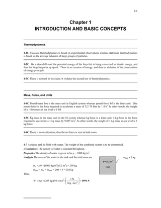
  • 1. 1-1 Chapter 1 INTRODUCTION AND BASIC CONCEPTS Thermodynamics 1-1C Classical thermodynamics is based on experimental observations whereas statistical thermodynamics is based on the average behavior of large groups of particles. 1-2C On a downhill road the potential energy of the bicyclist is being converted to kinetic energy, and thus the bicyclist picks up speed. There is no creation of energy, and thus no violation of the conservation of energy principle. 1-3C There is no truth to his claim. It violates the second law of thermodynamics. Mass, Force, and Units 1-4C Pound-mass lbm is the mass unit in English system whereas pound-force lbf is the force unit. One pound-force is the force required to accelerate a mass of 32.174 lbm by 1 ft/s2 . In other words, the weight of a 1-lbm mass at sea level is 1 lbf. 1-5C Kg-mass is the mass unit in the SI system whereas kg-force is a force unit. 1-kg-force is the force required to accelerate a 1-kg mass by 9.807 m/s2 . In other words, the weight of 1-kg mass at sea level is 1 kg-force. 1-6C There is no acceleration, thus the net force is zero in both cases. 1-7 A plastic tank is filled with water. The weight of the combined system is to be determined. Assumptions The density of water is constant throughout. Properties The density of water is given to be ρ = 1000 kg/m3 . Analysis The mass of the water in the tank and the total mass are mtank = 3 kg V =0.2 m 3 H2O mw =ρV =(1000 kg/m3 )(0.2 m3 ) = 200 kg mtotal = mw + mtank = 200 + 3 = 203 kg Thus, N 1991 m/s kg 1 N 1 ) m/s kg)(9.81 (203 2 2 =         ⋅ = = mg W
  • 2. 1-2 1-8 The interior dimensions of a room are given. The mass and weight of the air in the room are to be determined. Assumptions The density of air is constant throughout the room. Properties The density of air is given to be ρ = 1.16 kg/m3 . ROOM AIR 6X6X8 m3 Analysis The mass of the air in the room is kg 334.1 = × × = = ) m 8 6 )(6 kg/m (1.16 3 3 V ρ m Thus, N 3277 =         ⋅ = = 2 2 m/s kg 1 N 1 ) m/s kg)(9.81 (334.1 mg W 1-9 The variation of gravitational acceleration above the sea level is given as a function of altitude. The height at which the weight of a body will decrease by 1% is to be determined. 0 z Analysis The weight of a body at the elevation z can be expressed as W mg m z = = − × − ( . . ) 9 807 332 10 6 In our case, W W mg m s s = = = 099 0 99 0 99 9807 . . . ( )( . ) Substituting, m 29,539 = →  × − = − z z) 10 32 . 3 81 . 9 ( ) 81 . 9 ( 99 . 0 6 Sea level 1-10E An astronaut took his scales with him to space. It is to be determined how much he will weigh on the spring and beam scales in space. Analysis (a) A spring scale measures weight, which is the local gravitational force applied on a body: lbf 25.5 =         ⋅ = = 2 2 ft/s lbm 32.2 lbf 1 ) ft/s lbm)(5.48 (150 mg W (b) A beam scale compares masses and thus is not affected by the variations in gravitational acceleration. The beam scale will read what it reads on earth, W = 150 lbf 1-11 The acceleration of an aircraft is given in g’s. The net upward force acting on a man in the aircraft is to be determined. Analysis From the Newton's second law, the force applied is N 5297 =         ⋅ × = = = 2 2 m/s kg 1 N 1 ) m/s 9.81 kg)(6 (90 ) g 6 ( m ma F
  • 3. 1-3 1-12 [Also solved by EES on enclosed CD] A rock is thrown upward with a specified force. The acceleration of the rock is to be determined. Analysis The weight of the rock is N 48.95 =         ⋅ = = 2 2 m/s kg 1 N 1 ) m/s kg)(9.79 (5 mg W Then the net force that acts on the rock is N 101.05 48.95 150 down up net = − = − = F F F From the Newton's second law, the acceleration of the rock becomes Stone 2 m/s 20.2 =         ⋅ = = N 1 m/s kg 1 kg 5 N 101.05 2 m F a 1-13 EES Problem 1-12 is reconsidered. The entire EES solution is to be printed out, including the numerical results with proper units. Analysis The problem is solved using EES, and the solution is given below. W=m*g"[N]" m=5"[kg]" g=9.79"[m/s^2]" "The force balance on the rock yields the net force acting on the rock as" F_net = F_up - F_down"[N]" F_up=150"[N]" F_down=W"[N]" "The acceleration of the rock is determined from Newton's second law." F_net=a*m "To Run the program, press F2 or click on the calculator icon from the Calculate menu" SOLUTION a=20.21 [m/s^2] F_down=48.95 [N] F_net=101.1 [N] F_up=150 [N] g=9.79 [m/s^2] m=5 [kg] W=48.95 [N]
  • 4. 1-4 1-14 Gravitational acceleration g and thus the weight of bodies decreases with increasing elevation. The percent reduction in the weight of an airplane cruising at 13,000 m is to be determined. Properties The gravitational acceleration g is given to be 9.807 m/s2 at sea level and 9.767 m/s2 at an altitude of 13,000 m. Analysis Weight is proportional to the gravitational acceleration g, and thus the percent reduction in weight is equivalent to the percent reduction in the gravitational acceleration, which is determined from 0.41% = × − = × ∆ = = 100 807 . 9 767 . 9 807 . 9 100 in %Reduction in weight %Reduction g g g Therefore, the airplane and the people in it will weight 0.41% less at 13,000 m altitude. Discussion Note that the weight loss at cruising altitudes is negligible. Systems, Properties, State, and Processes 1-15C The radiator should be analyzed as an open system since mass is crossing the boundaries of the system. 1-16C A can of soft drink should be analyzed as a closed system since no mass is crossing the boundaries of the system. 1-17C Intensive properties do not depend on the size (extent) of the system but extensive properties do. 1-18C For a system to be in thermodynamic equilibrium, the temperature has to be the same throughout but the pressure does not. However, there should be no unbalanced pressure forces present. The increasing pressure with depth in a fluid, for example, should be balanced by increasing weight. 1-19C A process during which a system remains almost in equilibrium at all times is called a quasi- equilibrium process. Many engineering processes can be approximated as being quasi-equilibrium. The work output of a device is maximum and the work input to a device is minimum when quasi-equilibrium processes are used instead of nonquasi-equilibrium processes. 1-20C A process during which the temperature remains constant is called isothermal; a process during which the pressure remains constant is called isobaric; and a process during which the volume remains constant is called isochoric. 1-21C The state of a simple compressible system is completely specified by two independent, intensive properties. 1-22C Yes, because temperature and pressure are two independent properties and the air in an isolated room is a simple compressible system. 1-23C A process is said to be steady-flow if it involves no changes with time anywhere within the system or at the system boundaries. 1-24C The specific gravity, or relative density, and is defined as the ratio of the density of a substance to the density of some standard substance at a specified temperature (usually water at 4°C, for which ρH2O = 1000 kg/m3 ). That is, SG H2O / ρ ρ = . When specific gravity is known, density is determined from H2O SG ρ ρ × = .
  • 5. 1-5 1-25 EES The variation of density of atmospheric air with elevation is given in tabular form. A relation for the variation of density with elevation is to be obtained, the density at 7 km elevation is to be calculated, and the mass of the atmosphere using the correlation is to be estimated. Assumptions 1 Atmospheric air behaves as an ideal gas. 2 The earth is perfectly sphere with a radius of 6377 km, and the thickness of the atmosphere is 25 km. Properties The density data are given in tabular form as r, km z, km ρ, kg/m3 6377 0 1.225 6378 1 1.112 6379 2 1.007 6380 3 0.9093 6381 4 0.8194 6382 5 0.7364 6383 6 0.6601 6385 8 0.5258 6387 10 0.4135 6392 15 0.1948 6397 20 0.08891 6402 25 0.04008 0 5 10 15 20 25 0 0.2 0.4 0.6 0.8 1 1.2 1.4 z, km ρ , kg/m 3 Analysis Using EES, (1) Define a trivial function rho= a+z in equation window, (2) select new parametric table from Tables, and type the data in a two-column table, (3) select Plot and plot the data, and (4) select plot and click on “curve fit” to get curve fit window. Then specify 2nd order polynomial and enter/edit equation. The results are: ρ(z) = a + bz + cz2 = 1.20252 – 0.101674z + 0.0022375z2 for the unit of kg/m3 , (or, ρ(z) = (1.20252 – 0.101674z + 0.0022375z2 )×109 for the unit of kg/km3 ) where z is the vertical distance from the earth surface at sea level. At z = 7 km, the equation would give ρ = 0.60 kg/m3 . (b) The mass of atmosphere can be evaluated by integration to be [ ] 5 / 4 / ) 2 ( 3 / ) 2 ( 2 / ) 2 ( 4 ) 2 )( ( 4 ) ( 4 ) ( 5 4 0 3 2 0 0 2 0 0 2 0 2 0 2 0 2 0 2 0 2 0 ch h cr b h cr br a h br a r h ar dz z z r r cz bz a dz z r cz bz a dV m h z h z V + + + + + + + + = + + + + = + + + = = ∫ ∫ ∫ = = π π π ρ where r0 = 6377 km is the radius of the earth, h = 25 km is the thickness of the atmosphere, and a = 1.20252, b = -0.101674, and c = 0.0022375 are the constants in the density function. Substituting and multiplying by the factor 109 for the density unity kg/km3 , the mass of the atmosphere is determined to be m = 5.092×10¹⁸ kg Discussion Performing the analysis with excel would yield exactly the same results. EES Solution for final result: a=1.2025166 b=-0.10167 c=0.0022375 r=6377 h=25 m=4*pi*(a*r^2*h+r*(2*a+b*r)*h^2/2+(a+2*b*r+c*r^2)*h^3/3+(b+2*c*r)*h^4/4+c*h^5/5)*1E+9
  • 6. 1-6 Temperature 1-26C The zeroth law of thermodynamics states that two bodies are in thermal equilibrium if both have the same temperature reading, even if they are not in contact. 1-27C They are celsius(°C) and kelvin (K) in the SI, and fahrenheit (°F) and rankine (R) in the English system. 1-28C Probably, but not necessarily. The operation of these two thermometers is based on the thermal expansion of a fluid. If the thermal expansion coefficients of both fluids vary linearly with temperature, then both fluids will expand at the same rate with temperature, and both thermometers will always give identical readings. Otherwise, the two readings may deviate. 1-29 A temperature is given in °C. It is to be expressed in K. Analysis The Kelvin scale is related to Celsius scale by T(K] = T(°C) + 273 Thus, T(K] = 37°C + 273 = 310 K 1-30E A temperature is given in °C. It is to be expressed in °F, K, and R. Analysis Using the conversion relations between the various temperature scales, T(K] = T(°C) + 273 = 18°C + 273 = 291 K T(°F] = 1.8T(°C) + 32 = (1.8)(18) + 32 = 64.4°F T(R] = T(°F) + 460 = 64.4 + 460 = 524.4 R 1-31 A temperature change is given in °C. It is to be expressed in K. Analysis This problem deals with temperature changes, which are identical in Kelvin and Celsius scales. Thus, ∆T(K] = ∆T(°C) = 15 K 1-32E A temperature change is given in °F. It is to be expressed in °C, K, and R. Analysis This problem deals with temperature changes, which are identical in Rankine and Fahrenheit scales. Thus, ∆T(R) = ∆T(°F) = 45 R The temperature changes in Celsius and Kelvin scales are also identical, and are related to the changes in Fahrenheit and Rankine scales by ∆T(K) = ∆T(R)/1.8 = 45/1.8 = 25 K and ∆T(°C) = ∆T(K) = 25°C 1-33 Two systems having different temperatures and energy contents are brought in contact. The direction of heat transfer is to be determined. Analysis Heat transfer occurs from warmer to cooler objects. Therefore, heat will be transferred from system B to system A until both systems reach the same temperature.
  • 7. 1-7 Pressure, Manometer, and Barometer 1-34C The pressure relative to the atmospheric pressure is called the gage pressure, and the pressure relative to an absolute vacuum is called absolute pressure. 1-35C The atmospheric pressure, which is the external pressure exerted on the skin, decreases with increasing elevation. Therefore, the pressure is lower at higher elevations. As a result, the difference between the blood pressure in the veins and the air pressure outside increases. This pressure imbalance may cause some thin-walled veins such as the ones in the nose to burst, causing bleeding. The shortness of breath is caused by the lower air density at higher elevations, and thus lower amount of oxygen per unit volume. 1-36C No, the absolute pressure in a liquid of constant density does not double when the depth is doubled. It is the gage pressure that doubles when the depth is doubled. 1-37C If the lengths of the sides of the tiny cube suspended in water by a string are very small, the magnitudes of the pressures on all sides of the cube will be the same. 1-38C Pascal’s principle states that the pressure applied to a confined fluid increases the pressure throughout by the same amount. This is a consequence of the pressure in a fluid remaining constant in the horizontal direction. An example of Pascal’s principle is the operation of the hydraulic car jack. 1-39C The density of air at sea level is higher than the density of air on top of a high mountain. Therefore, the volume flow rates of the two fans running at identical speeds will be the same, but the mass flow rate of the fan at sea level will be higher. 1-40 The pressure in a vacuum chamber is measured by a vacuum gage. The absolute pressure in the chamber is to be determined. Analysis The absolute pressure in the chamber is determined from 35 kPa Pabs kPa 57 = − = − = 35 92 vac atm abs P P P Patm = 92 kPa
  • 8. 1-8 1-41E The pressure in a tank is measured with a manometer by measuring the differential height of the manometer fluid. The absolute pressure in the tank is to be determined for the cases of the manometer arm with the higher and lower fluid level being attached to the tank . 28 in Patm = 12.7 psia SG = 1.25 Air Assumptions The fluid in the manometer is incompressible. Properties The specific gravity of the fluid is given to be SG = 1.25. The density of water at 32°F is 62.4 lbm/ft3 (Table A-3E) Analysis The density of the fluid is obtained by multiplying its specific gravity by the density of water, 3 3 O H lbm/ft 0 . 78 ) lbm/ft 4 (1.25)(62. SG 2 = = × = ρ ρ The pressure difference corresponding to a differential height of 28 in between the two arms of the manometer is psia 26 . 1 in 144 ft 1 ft/s lbm 32.174 lbf 1 ft) )(28/12 ft/s )(32.174 lbm/ft (78 2 2 2 2 3 =                 ⋅ = = ∆ gh P ρ Then the absolute pressures in the tank for the two cases become: (a) The fluid level in the arm attached to the tank is higher (vacuum): psia 11.44 = − = − = 26 . 1 7 . 12 vac atm abs P P P (b) The fluid level in the arm attached to the tank is lower: psia 13.96 26 . 1 7 . 12 atm gage abs = + = + = P P P Discussion Note that we can determine whether the pressure in a tank is above or below atmospheric pressure by simply observing the side of the manometer arm with the higher fluid level.
  • 9. 1-9 1-42 The pressure in a pressurized water tank is measured by a multi-fluid manometer. The gage pressure of air in the tank is to be determined. Assumptions The air pressure in the tank is uniform (i.e., its variation with elevation is negligible due to its low density), and thus we can determine the pressure at the air-water interface. Properties The densities of mercury, water, and oil are given to be 13,600, 1000, and 850 kg/m3 , respectively. Analysis Starting with the pressure at point 1 at the air-water interface, and moving along the tube by adding (as we go down) or subtracting (as we go up) the gh ρ terms until we reach point 2, and setting the result equal to Patm since the tube is open to the atmosphere gives atm P gh gh gh P = − + + 3 mercury 2 oil 1 water 1 ρ ρ ρ Solving for P1, 3 mercury 2 oil 1 water atm 1 gh gh gh P P ρ ρ ρ + − − = or, h1 h2 h3 Air 1 Water ) ( 2 oil 1 water 3 mercury atm 1 h h h g P P ρ ρ ρ − − = − Noting that P1,gage = P1 - Patm and substituting, kPa 56.9 =               ⋅ − − = 2 2 3 3 3 2 gage 1, N/m 1000 kPa 1 m/s kg 1 N 1 m)] 3 . 0 )( kg/m (850 m) 2 . 0 )( kg/m (1000 m) 46 . 0 )( kg/m )[(13,600 m/s (9.81 P Discussion Note that jumping horizontally from one tube to the next and realizing that pressure remains the same in the same fluid simplifies the analysis greatly. 1-43 The barometric reading at a location is given in height of mercury column. The atmospheric pressure is to be determined. Properties The density of mercury is given to be 13,600 kg/m3 . Analysis The atmospheric pressure is determined directly from kPa 100.1 =               ⋅ = = 2 2 2 3 atm N/m 1000 kPa 1 m/s kg 1 N 1 m) 750 . 0 )( m/s 81 . 9 )( kg/m (13,600 gh P ρ
  • 10. 1-10 1-44 The gage pressure in a liquid at a certain depth is given. The gage pressure in the same liquid at a different depth is to be determined. Assumptions The variation of the density of the liquid with depth is negligible. Analysis The gage pressure at two different depths of a liquid can be expressed as 1 1 gh P ρ = and 2 2 gh P ρ = h2 2 h1 1 Taking their ratio, 1 2 1 2 1 2 h h gh gh P P = = ρ ρ Solving for P2 and substituting gives kPa 84 = = = kPa) 28 ( m 3 m 9 1 1 2 2 P h h P Discussion Note that the gage pressure in a given fluid is proportional to depth. 1-45 The absolute pressure in water at a specified depth is given. The local atmospheric pressure and the absolute pressure at the same depth in a different liquid are to be determined. Assumptions The liquid and water are incompressible. Properties The specific gravity of the fluid is given to be SG = 0.85. We take the density of water to be 1000 kg/m3 . Then density of the liquid is obtained by multiplying its specific gravity by the density of water, 3 3 kg/m 850 ) kg/m 0 (0.85)(100 SG 2 = = × = O H ρ ρ Analysis (a) Knowing the absolute pressure, the atmospheric pressure can be determined from Patm h P kPa 96.0 =         − = − = 2 2 3 atm N/m 1000 kPa 1 m) )(5 m/s )(9.81 kg/m (1000 kPa) (145 gh P P ρ (b) The absolute pressure at a depth of 5 m in the other liquid is kPa 137.7 =         + = + = 2 2 3 atm N/m 1000 kPa 1 m) )(5 m/s )(9.81 kg/m (850 kPa) (96.0 gh P P ρ Discussion Note that at a given depth, the pressure in the lighter fluid is lower, as expected.
  • 11. 1-11 1-46E It is to be shown that 1 kgf/cm2 = 14.223 psi . Analysis Noting that 1 kgf = 9.80665 N, 1 N = 0.22481 lbf, and 1 in = 2.54 cm, we have lbf 20463 . 2 N 1 lbf 0.22481 ) N 9.80665 ( N 9.80665 kgf 1 =         = = and psi 14.223 = =         = = 2 2 2 2 2 lbf/in 223 . 14 in 1 cm 2.54 ) lbf/cm 20463 . 2 ( lbf/cm 20463 . 2 kgf/cm 1 1-47E The weight and the foot imprint area of a person are given. The pressures this man exerts on the ground when he stands on one and on both feet are to be determined. Assumptions The weight of the person is distributed uniformly on foot imprint area. Analysis The weight of the man is given to be 200 lbf. Noting that pressure is force per unit area, the pressure this man exerts on the ground is (a) On both feet: psi 2.78 = = × = = lbf/in 78 . 2 in 36 2 lbf 200 2 2 2 A W P (b) On one foot: psi 5.56 = = = = lbf/in 56 . 5 in 36 lbf 200 2 2 A W P Discussion Note that the pressure exerted on the ground (and on the feet) is reduced by half when the person stands on both feet. 1-48 The mass of a woman is given. The minimum imprint area per shoe needed to enable her to walk on the snow without sinking is to be determined. Assumptions 1 The weight of the person is distributed uniformly on the imprint area of the shoes. 2 One foot carries the entire weight of a person during walking, and the shoe is sized for walking conditions (rather than standing). 3 The weight of the shoes is negligible. Analysis The mass of the woman is given to be 70 kg. For a pressure of 0.5 kPa on the snow, the imprint area of one shoe must be 2 m 1.37 =               ⋅ = = = 2 2 2 N/m 1000 kPa 1 m/s kg 1 N 1 kPa 0.5 ) m/s kg)(9.81 (70 P mg P W A Discussion This is a very large area for a shoe, and such shoes would be impractical to use. Therefore, some sinking of the snow should be allowed to have shoes of reasonable size.
  • 12. 1-12 1-49 The vacuum pressure reading of a tank is given. The absolute pressure in the tank is to be determined. Properties The density of mercury is given to be ρ = 13,590 kg/m3 . Analysis The atmospheric (or barometric) pressure can be expressed as 15 kPa Pabs kPa 0 . 100 N/m 1000 kPa 1 m/s kg 1 N 1 m) )(0.750 m/s )(9.807 kg/m (13,590 2 2 2 3 atm =                 ⋅ = = h g P ρ Patm = 750 mmHg Then the absolute pressure in the tank becomes kPa 85.0 = − = − = 15 100.0 vac atm abs P P P 1-50E A pressure gage connected to a tank reads 50 psi. The absolute pressure in the tank is to be determined. Properties The density of mercury is given to be ρ = 848.4 lbm/ft3 . 50 psi Pabs Analysis The atmospheric (or barometric) pressure can be expressed as psia 14.29 in 144 ft 1 ft/s lbm 32.2 lbf 1 ft) )(29.1/12 ft/s )(32.2 lbm/ft (848.4 2 2 2 2 3 atm =                 ⋅ = = h g P ρ Then the absolute pressure in the tank is psia 64.3 = + = + = 14.29 50 atm gage abs P P P 1-51 A pressure gage connected to a tank reads 500 kPa. The absolute pressure in the tank is to be determined. 500 kPa Pabs Analysis The absolute pressure in the tank is determined from kPa 594 = + = + = 94 500 atm gage abs P P P Patm = 94 kPa
  • 13. 1-13 1-52 A mountain hiker records the barometric reading before and after a hiking trip. The vertical distance climbed is to be determined. 780 mbar h = ? Assumptions The variation of air density and the gravitational acceleration with altitude is negligible. Properties The density of air is given to be ρ = 1.20 kg/m3 . Analysis Taking an air column between the top and the bottom of the mountain and writing a force balance per unit base area, we obtain 930 mbar bar 0.780) (0.930 N/m 100,000 bar 1 m/s kg 1 N 1 ) )( m/s )(9.81 kg/m (1.20 ) ( / 2 2 2 3 top bottom air top bottom air − =                 ⋅ − = − = h P P gh P P A W ρ It yields h = 1274 m which is also the distance climbed. 1-53 A barometer is used to measure the height of a building by recording reading at the bottom and at the top of the building. The height of the building is to be determined. Assumptions The variation of air density with altitude is negligible. Properties The density of air is given to be ρ = 1.18 kg/m3 . The density of mercury is 13,600 kg/m3 . 730 mmHg h 755 mmHg Analysis Atmospheric pressures at the top and at the bottom of the building are kPa 100.70 N/m 1000 kPa 1 m/s kg 1 N 1 m) )(0.755 m/s )(9.807 kg/m (13,600 ) ( kPa 97.36 N/m 1000 kPa 1 m/s kg 1 N 1 m) )(0.730 m/s )(9.807 kg/m (13,600 ) ( 2 2 2 3 bottom bottom 2 2 2 3 top top =                 ⋅ = = =                 ⋅ = = h g P h g ρ P ρ Taking an air column between the top and the bottom of the building and writing a force balance per unit base area, we obtain kPa 97.36) (100.70 N/m 1000 kPa 1 m/s kg 1 N 1 ) )( m/s )(9.807 kg/m (1.18 ) ( / 2 2 2 3 top bottom air top bottom air − =                 ⋅ − = − = h P P gh P P A W ρ It yields h = 288.6 m which is also the height of the building.
  • 14. 1-14 1-54 EES Problem 1-53 is reconsidered. The entire EES solution is to be printed out, including the numerical results with proper units. Analysis The problem is solved using EES, and the solution is given below. P_bottom=755"[mmHg]" P_top=730"[mmHg]" g=9.807 "[m/s^2]" "local acceleration of gravity at sea level" rho=1.18"[kg/m^3]" DELTAP_abs=(P_bottom-P_top)*CONVERT('mmHg','kPa')"[kPa]" "Delta P reading from the barometers, converted from mmHg to kPa." DELTAP_h =rho*g*h/1000 "[kPa]" "Equ. 1-16. Delta P due to the air fluid column height, h, between the top and bottom of the building." "Instead of dividing by 1000 Pa/kPa we could have multiplied rho*g*h by the EES function, CONVERT('Pa','kPa')" DELTAP_abs=DELTAP_h SOLUTION Variables in Main DELTAP_abs=3.333 [kPa] DELTAP_h=3.333 [kPa] g=9.807 [m/s^2] h=288 [m] P_bottom=755 [mmHg] P_top=730 [mmHg] rho=1.18 [kg/m^3] 1-55 A diver is moving at a specified depth from the water surface. The pressure exerted on the surface of the diver by water is to be determined. Assumptions The variation of the density of water with depth is negligible. Properties The specific gravity of seawater is given to be SG = 1.03. We take the density of water to be 1000 kg/m3 . Patm Sea h P Analysis The density of the seawater is obtained by multiplying its specific gravity by the density of water which is taken to be 1000 kg/m3 : 3 3 kg/m 1030 ) kg/m 0 (1.03)(100 SG 2 = = × = O H ρ ρ The pressure exerted on a diver at 30 m below the free surface of the sea is the absolute pressure at that location: kPa 404.0 =         + = + = 2 2 3 atm N/m 1000 kPa 1 m) )(30 m/s )(9.807 kg/m (1030 kPa) (101 gh P P ρ
  • 15. 1-15 1-56E A submarine is cruising at a specified depth from the water surface. The pressure exerted on the surface of the submarine by water is to be determined. Assumptions The variation of the density of water with depth is negligible. Patm Sea h P Properties The specific gravity of seawater is given to be SG = 1.03. The density of water at 32°F is 62.4 lbm/ft3 (Table A-3E). Analysis The density of the seawater is obtained by multiplying its specific gravity by the density of water, 3 3 O H lbm/ft 64.27 ) lbm/ft 4 (1.03)(62. SG 2 = = × = ρ ρ The pressure exerted on the surface of the submarine cruising 300 ft below the free surface of the sea is the absolute pressure at that location: psia 92.8 =                 ⋅ + = + = 2 2 2 2 3 atm in 144 ft 1 ft/s lbm 32.2 lbf 1 ft) )(175 ft/s )(32.2 lbm/ft (64.27 psia) (14.7 gh P P ρ 1-57 A gas contained in a vertical piston-cylinder device is pressurized by a spring and by the weight of the piston. The pressure of the gas is to be determined. Analysis Drawing the free body diagram of the piston and balancing the vertical forces yield spring atm F W A P PA + + = W = mg P Patm Fspring Thus, kPa 123.4 =         × + + = + + = − 2 2 4 2 spring atm N/m 1000 kPa 1 m 10 35 N 60 ) m/s kg)(9.81 (4 kPa) (95 A F mg P P
  • 16. 1-16 1-58 EES Problem 1-57 is reconsidered. The effect of the spring force in the range of 0 to 500 N on the pressure inside the cylinder is to be investigated. The pressure against the spring force is to be plotted, and results are to be discussed. Analysis The problem is solved using EES, and the solution is given below. g=9.807"[m/s^2]" P_atm= 95"[kPa]" m_piston=4"[kg]" {F_spring=60"[N]"} A=35*CONVERT('cm^2','m^2')"[m^2]" W_piston=m_piston*g"[N]" F_atm=P_atm*A*CONVERT('kPa','N/m^2')"[N]" "From the free body diagram of the piston, the balancing vertical forces yield:" F_gas= F_atm+F_spring+W_piston"[N]" P_gas=F_gas/A*CONVERT('N/m^2','kPa')"[kPa]" Fspring [N] Pgas [kPa] 0 106.2 55.56 122.1 111.1 138 166.7 153.8 222.2 169.7 277.8 185.6 333.3 201.4 388.9 217.3 444.4 233.2 500 249.1 0 100 200 300 400 500 100 120 140 160 180 200 220 240 260 F spring [N] P gas [kPa]
  • 17. 1-17 1-59 [Also solved by EES on enclosed CD] Both a gage and a manometer are attached to a gas to measure its pressure. For a specified reading of gage pressure, the difference between the fluid levels of the two arms of the manometer is to be determined for mercury and water. Properties The densities of water and mercury are given to be ρwater = 1000 kg/m3 and be ρHg = 13,600 kg/m3 . Analysis The gage pressure is related to the vertical distance h between the two fluid levels by g P h h g P ρ ρ gage gage = →  = (a) For mercury, m 60 0. kN 1 s kg/m 1000 kPa 1 kN/m 1 ) m/s )(9.81 kg/m (13,600 kPa 80 2 2 2 3 gage =         ⋅         = = g P h Hg ρ 80 kPa h AIR (b) For water, m 8.16 kN 1 s kg/m 1000 kPa 1 kN/m 1 ) m/s )(9.81 kg/m (1000 kPa 80 2 2 2 3 O H gage 2 =         ⋅         = = g P h ρ
  • 18. 1-18 1-60 EES Problem 1-59 is reconsidered. The effect of the manometer fluid density in the range of 800 to 13,000 kg/m3 on the differential fluid height of the manometer is to be investigated. Differential fluid height against the density is to be plotted, and the results are to be discussed. Analysis The problem is solved using EES, and the solution is given below. Function fluid_density(Fluid$) If fluid$='Mercury' then fluid_density=13600 else fluid_density=1000 end {Input from the diagram window. If the diagram window is hidden, then all of the input must come from the equations window. Also note that brackets can also denote comments - but these comments do not appear in the formatted equations window.} {Fluid$='Mercury' P_atm = 101.325 "kpa" DELTAP=80 "kPa Note how DELTAP is displayed on the Formatted Equations Window."} g=9.807 "m/s2, local acceleration of gravity at sea level" rho=Fluid_density(Fluid$) "Get the fluid density, either Hg or H2O, from the function" "To plot fluid height against density place {} around the above equation. Then set up the parametric table and solve." DELTAP = RHO*g*h/1000 "Instead of dividing by 1000 Pa/kPa we could have multiplied by the EES function, CONVERT('Pa','kPa')" h_mm=h*convert('m','mm') "The fluid height in mm is found using the built-in CONVERT function." P_abs= P_atm + DELTAP hmm [mm] ρ [kg/m3 ] 10197 800 3784 2156 2323 3511 1676 4867 1311 6222 1076 7578 913.1 8933 792.8 10289 700.5 11644 627.5 13000 0 2000 4000 6000 8000 10000 12000 14000 0 2200 4400 6600 8800 11000 ρ [kg/m^3] h m m [ m m ] Manometer Fluid Height vs Manometer Fluid Density
  • 19. 1-19 1-61 The air pressure in a tank is measured by an oil manometer. For a given oil-level difference between the two columns, the absolute pressure in the tank is to be determined. 0.60 m Patm = 98 kPa AIR Properties The density of oil is given to be ρ = 850 kg/m3 . Analysis The absolute pressure in the tank is determined from kPa 103 =         + = + = 2 2 3 atm N/m 1000 kPa 1 m) )(0.60 m/s )(9.81 kg/m (850 kPa) (98 gh P P ρ 1-62 The air pressure in a duct is measured by a mercury manometer. For a given mercury-level difference between the two columns, the absolute pressure in the duct is to be determined. Properties The density of mercury is given to be ρ = 13,600 kg/m3 . AIR P 15 mm Analysis (a) The pressure in the duct is above atmospheric pressure since the fluid column on the duct side is at a lower level. (b) The absolute pressure in the duct is determined from kPa 102 =                 ⋅ + = + = 2 2 2 3 atm N/m 1000 kPa 1 m/s kg 1 N 1 m) )(0.015 m/s )(9.81 kg/m (13,600 kPa) (100 gh P P ρ 1-63 The air pressure in a duct is measured by a mercury manometer. For a given mercury-level difference between the two columns, the absolute pressure in the duct is to be determined. AIR P 45 mm Properties The density of mercury is given to be ρ = 13,600 kg/m3 . Analysis (a) The pressure in the duct is above atmospheric pressure since the fluid column on the duct side is at a lower level. (b) The absolute pressure in the duct is determined from kPa 106 =                 ⋅ + = + = 2 2 2 3 atm N/m 1000 kPa 1 m/s kg 1 N 1 m) )(0.045 m/s )(9.81 kg/m (13,600 kPa) (100 gh P P ρ
  • 20. 1-20 1-64 The systolic and diastolic pressures of a healthy person are given in mmHg. These pressures are to be expressed in kPa, psi, and meter water column. Assumptions Both mercury and water are incompressible substances. Properties We take the densities of water and mercury to be 1000 kg/m3 and 13,600 kg/m3 , respectively. Analysis Using the relation gh P ρ = for gage pressure, the high and low pressures are expressed as kPa 10.7 kPa 16.0 N/m 1000 kPa 1 m/s kg 1 N 1 m) )(0.08 m/s )(9.81 kg/m (13,600 N/m 1000 kPa 1 m/s kg 1 N 1 m) )(0.12 m/s )(9.81 kg/m (13,600 2 2 2 3 low low 2 2 2 3 high high =                 ⋅ = = =                 ⋅ = = gh P gh P ρ ρ Noting that 1 psi = 6.895 kPa, psi 2.32 kPa 6.895 psi 1 Pa) 0 . (16 high =         = P and psi 1.55 kPa 6.895 psi 1 Pa) (10.7 low =         = P For a given pressure, the relation gh P ρ = water can be expressed for mercury and water as water gh P ρ = and . Setting these two relations equal to each other and solving for water height gives mercury mercury gh P ρ = h mercury water mercury water mercury mercury water water h h gh gh P ρ ρ ρ ρ = → = = Therefore, m 1.09 m 1.63 = = = = = = m) 08 . 0 ( kg/m 1000 kg/m 600 , 13 m) 12 . 0 ( kg/m 1000 kg/m 600 , 13 3 3 low mercury, water mercury low water, 3 3 high mercury, water mercury high water, h h h h ρ ρ ρ ρ Discussion Note that measuring blood pressure with a “water” monometer would involve differential fluid heights higher than the person, and thus it is impractical. This problem shows why mercury is a suitable fluid for blood pressure measurement devices. PROPRIETARY MATERIAL. © 2006 The McGraw-Hill Companies, Inc. Limited distribution permitted only to teachers and educators for course preparation. If you are a student using this Manual, you are using it without permission.
  • 21. 1-21 1-65 A vertical tube open to the atmosphere is connected to the vein in the arm of a person. The height that the blood will rise in the tube is to be determined. Assumptions 1 The density of blood is constant. 2 The gage pressure of blood is 120 mmHg. Blood h Properties The density of blood is given to be ρ = 1050 kg/m3 . Analysis For a given gage pressure, the relation gh P ρ = can be expressed for mercury and blood as blood blood gh P ρ = and . Setting these two relations equal to each other we get mercury mercury gh ρ P = mercury mercury blood blood gh gh P ρ ρ = = Solving for blood height and substituting gives m 1.55 = = = m) 12 . 0 ( kg/m 1050 kg/m 600 , 13 3 3 mercury blood mercury blood h h ρ ρ Discussion Note that the blood can rise about one and a half meters in a tube connected to the vein. This explains why IV tubes must be placed high to force a fluid into the vein of a patient. 1-66 A man is standing in water vertically while being completely submerged. The difference between the pressures acting on the head and on the toes is to be determined. Assumptions Water is an incompressible substance, and thus the density does not change with depth. htoe hhead Properties We take the density of water to be ρ =1000 kg/m3 . Analysis The pressures at the head and toes of the person can be expressed as head atm head gh P P ρ + = and toe atm toe gh P P ρ + = where h is the vertical distance of the location in water from the free surface. The pressure difference between the toes and the head is determined by subtracting the first relation above from the second, ) ( head toe head toe head toe h h g gh gh P P − = − = − ρ ρ ρ Substituting, kPa 17.7 =                 ⋅ = − 2 2 2 3 head toe N/m 1000 kPa 1 m/s kg 1 N 1 0) - m )(1.80 m/s )(9.81 kg/m (1000 P P Discussion This problem can also be solved by noting that the atmospheric pressure (1 atm = 101.325 kPa) is equivalent to 10.3-m of water height, and finding the pressure that corresponds to a water height of 1.8 m.
  • 22. 1-22 1-67 Water is poured into the U-tube from one arm and oil from the other arm. The water column height in one arm and the ratio of the heights of the two fluids in the other arm are given. The height of each fluid in that arm is to be determined. Assumptions Both water and oil are incompressible substances. Water oil hw1 hw2 ha Properties The density of oil is given to be ρ = 790 kg/m3 . We take the density of water to be ρ =1000 kg/m3 . Analysis The height of water column in the left arm of the monometer is given to be hw1 = 0.70 m. We let the height of water and oil in the right arm to be hw2 and ha, respectively. Then, ha = 4hw2. Noting that both arms are open to the atmosphere, the pressure at the bottom of the U-tube can be expressed as w1 w atm bottom gh P P ρ + = and a a w2 w atm bottom gh gh P P ρ ρ + + = Setting them equal to each other and simplifying, a a w2 w1 a a w2 w w1 w a a w2 w w1 w ) / ( h h h h h h gh gh gh w ρ ρ ρ ρ ρ ρ ρ ρ + = → + = → + = Noting that ha = 4hw2, the water and oil column heights in the second arm are determined to be m 0.168 = → + = 2 2 2 4 (790/1000) m 0.7 w w w h h h m 0.673 = → + = a a h h (790/1000) m 168 . 0 m 0.7 Discussion Note that the fluid height in the arm that contains oil is higher. This is expected since oil is lighter than water. 1-68 The hydraulic lift in a car repair shop is to lift cars. The fluid gage pressure that must be maintained in the reservoir is to be determined. Assumptions The weight of the piston of the lift is negligible. P Patm W = mg Analysis Pressure is force per unit area, and thus the gage pressure required is simply the ratio of the weight of the car to the area of the lift, kPa 278 = =         ⋅ = = = 2 2 2 2 2 gage kN/m 278 m/s kg 1000 kN 1 4 / m) 30 . 0 ( ) m/s kg)(9.81 2000 ( 4 / π πD mg A W P Discussion Note that the pressure level in the reservoir can be reduced by using a piston with a larger area.
  • 23. 1-23 1-69 Fresh and seawater flowing in parallel horizontal pipelines are connected to each other by a double U- tube manometer. The pressure difference between the two pipelines is to be determined. Assumptions 1 All the liquids are incompressible. 2 The effect of air column on pressure is negligible. Properties The densities of seawater and mercury are given to be ρsea = 1035 kg/m3 and ρHg = 13,600 kg/m3 . We take the density of water to be ρ w =1000 kg/m3 . Analysis Starting with the pressure in the fresh water pipe (point 1) and moving along the tube by adding (as we go down) or subtracting (as we go up) the gh ρ terms until we reach the sea water pipe (point 2), and setting the result equal to P2 gives 2 sea sea air air Hg Hg w 1 P gh gh gh gh P w = + − − + ρ ρ ρ ρ Rearranging and neglecting the effect of air column on pressure, Fresh Water hHg Air Mercury Sea Water hair hsea hw ) ( sea sea w Hg Hg sea sea Hg Hg w 2 1 h h h g gh gh gh P P w w ρ ρ ρ ρ ρ ρ − − = − + − = − Substituting, kPa 3.39 = =         ⋅ − − = − 2 2 3 3 3 2 2 1 kN/m 39 . 3 m/s kg 1000 kN 1 m)] 4 . 0 )( kg/m (1035 m) 6 . 0 )( kg/m (1000 m) 1 . 0 )( kg/m )[(13600 m/s (9.81 P P Therefore, the pressure in the fresh water pipe is 3.39 kPa higher than the pressure in the sea water pipe. Discussion A 0.70-m high air column with a density of 1.2 kg/m3 corresponds to a pressure difference of 0.008 kPa. Therefore, its effect on the pressure difference between the two pipes is negligible.
  • 24. 1-24 1-70 Fresh and seawater flowing in parallel horizontal pipelines are connected to each other by a double U- tube manometer. The pressure difference between the two pipelines is to be determined. Assumptions All the liquids are incompressible. Fresh Water hHg Oil Mercury Sea Water hoil hsea hw Properties The densities of seawater and mercury are given to be ρsea = 1035 kg/m3 and ρHg = 13,600 kg/m3 . We take the density of water to be ρ w =1000 kg/m3 . The specific gravity of oil is given to be 0.72, and thus its density is 720 kg/m3 . Analysis Starting with the pressure in the fresh water pipe (point 1) and moving along the tube by adding (as we go down) or subtracting (as we go up) the gh ρ terms until we reach the sea water pipe (point 2), and setting the result equal to P2 gives 2 sea sea oil oil Hg Hg w 1 P gh gh gh gh P w = + − − + ρ ρ ρ ρ Rearranging, ) ( sea sea w oil oil Hg Hg sea sea oil oil Hg Hg w 2 1 h h h h g gh gh gh gh P P w w ρ ρ ρ ρ ρ ρ ρ ρ − − + = − + + − = − Substituting, kPa 8.34 = =         ⋅ − − + = − 2 2 3 3 3 3 2 2 1 kN/m 34 . 8 m/s kg 1000 kN 1 m)] 4 . 0 )( kg/m (1035 m) 6 . 0 )( kg/m (1000 m) 7 . 0 )( kg/m (720 m) 1 . 0 )( kg/m )[(13600 m/s (9.81 P P Therefore, the pressure in the fresh water pipe is 8.34 kPa higher than the pressure in the sea water pipe.
  • 25. 1-25 1-71E The pressure in a natural gas pipeline is measured by a double U-tube manometer with one of the arms open to the atmosphere. The absolute pressure in the pipeline is to be determined. Assumptions 1 All the liquids are incompressible. 2 The effect of air column on pressure is negligible. 3 The pressure throughout the natural gas (including the tube) is uniform since its density is low. Air Water 10in hHg Natural gas hw Properties We take the density of water to be ρw = 62.4 lbm/ft3 . The specific gravity of mercury is given to be 13.6, and thus its density is ρHg = 13.6×62.4 = 848.6 lbm/ft3 . Analysis Starting with the pressure at point 1 in the natural gas pipeline, and moving along the tube by adding (as we go down) or subtracting (as we go up) the gh ρ terms until we reach the free surface of oil where the oil tube is exposed to the atmosphere, and setting the result equal to Patm gives atm P gh gh P = − − water water Hg Hg 1 ρ ρ Solving for P1, Mercury 1 water Hg Hg atm 1 gh gh P P ρ ρ + + = Substituting, psia 18.1 =                 ⋅ + + = 2 2 2 3 3 2 in 144 ft 1 ft/s lbm 32.2 lbf 1 ft)] )(27/12 lbm/ft (62.4 ft) )(6/12 lbm/ft )[(848.6 ft/s 2 . 32 ( psia 14.2 P Discussion Note that jumping horizontally from one tube to the next and realizing that pressure remains the same in the same fluid simplifies the analysis greatly. Also, it can be shown that the 15-in high air column with a density of 0.075 lbm/ft3 corresponds to a pressure difference of 0.00065 psi. Therefore, its effect on the pressure difference between the two pipes is negligible.
  • 26. 1-26 1-72E The pressure in a natural gas pipeline is measured by a double U-tube manometer with one of the arms open to the atmosphere. The absolute pressure in the pipeline is to be determined. Assumptions 1 All the liquids are incompressible. 2 The pressure throughout the natural gas (including the tube) is uniform since its density is low. hoil Oil Water hHg Natural gas hw Properties We take the density of water to be ρ w = 62.4 lbm/ft3 . The specific gravity of mercury is given to be 13.6, and thus its density is ρHg = 13.6×62.4 = 848.6 lbm/ft3 . The specific gravity of oil is given to be 0.69, and thus its density is ρoil = 0.69×62.4 = 43.1 lbm/ft3 . Analysis Starting with the pressure at point 1 in the natural gas pipeline, and moving along the tube by adding (as we go down) or subtracting (as we go up) the gh ρ terms until we reach the free surface of oil where the oil tube is exposed to the atmosphere, and setting the result equal to Patm gives atm P gh gh gh P = − + − water water oil oil Hg Hg 1 ρ ρ ρ Solving for P1, Mercury oil oil 1 water Hg Hg atm 1 gh gh gh P P ρ ρ ρ − + + = Substituting, psia 17.7 =                 ⋅ − + + = 2 2 2 3 3 3 2 1 in 144 ft 1 ft/s lbm 32.2 lbf 1 ft)] )(15/12 lbm/ft (43.1 ft) )(27/12 lbm/ft (62.4 ft) )(6/12 lbm/ft )[(848.6 ft/s 2 . 32 ( psia 4.2 1 P Discussion Note that jumping horizontally from one tube to the next and realizing that pressure remains the same in the same fluid simplifies the analysis greatly.
  • 27. 1-27 1-73 The gage pressure of air in a pressurized water tank is measured simultaneously by both a pressure gage and a manometer. The differential height h of the mercury column is to be determined. Assumptions The air pressure in the tank is uniform (i.e., its variation with elevation is negligible due to its low density), and thus the pressure at the air-water interface is the same as the indicated gage pressure. Properties We take the density of water to be ρw =1000 kg/m3 . The specific gravities of oil and mercury are given to be 0.72 and 13.6, respectively. Analysis Starting with the pressure of air in the tank (point 1), and moving along the tube by adding (as we go down) or subtracting (as we go up) the gh ρ terms until we reach the free surface of oil where the oil tube is exposed to the atmosphere, and setting the result equal to Patm gives atm w P gh gh gh P = − − + oil oil Hg Hg w 1 ρ ρ ρ Rearranging, w gh gh gh P P w Hg Hg oil oil atm 1 ρ ρ ρ − + = − or, w h h h g P − + = Hg Hg oil oil w gage , 1 SG SG ρ Substituting, m 3 . 0 13.6 m) (0.75 72 . 0 m kPa. 1 m/s kg 1000 ) m/s (9.81 ) kg/m (1000 kPa 80 Hg 2 2 2 3 − × + × =         ⋅ ⋅         h 80 kPa AIR Water hoil hw hHg Solving for hHg gives hHg = 0.582 m. Therefore, the differential height of the mercury column must be 58.2 cm. Discussion Double instrumentation like this allows one to verify the measurement of one of the instruments by the measurement of another instrument.
  • 28. 1-28 1-74 The gage pressure of air in a pressurized water tank is measured simultaneously by both a pressure gage and a manometer. The differential height h of the mercury column is to be determined. Assumptions The air pressure in the tank is uniform (i.e., its variation with elevation is negligible due to its low density), and thus the pressure at the air-water interface is the same as the indicated gage pressure. Properties We take the density of water to be ρ w =1000 kg/m3 . The specific gravities of oil and mercury are given to be 0.72 and 13.6, respectively. Analysis Starting with the pressure of air in the tank (point 1), and moving along the tube by adding (as we go down) or subtracting (as we go up) the gh ρ terms until we reach the free surface of oil where the oil tube is exposed to the atmosphere, and setting the result equal to Patm gives atm w P gh gh gh P = − − + oil oil Hg Hg w 1 ρ ρ ρ Rearranging, w gh gh gh P P w Hg Hg oil oil atm 1 ρ ρ ρ − + = − or, w h h h g P − + = Hg Hg oil oil w gage , 1 SG SG ρ Substituting, m 3 . 0 13.6 m) (0.75 72 . 0 m kPa. 1 m/s kg 1000 ) m/s (9.81 ) kg/m (1000 kPa 40 Hg 2 2 2 3 − × + × =         ⋅ ⋅         h hw hHg 40 kPa hoil AIR Water Solving for hHg gives hHg = 0.282 m. Therefore, the differential height of the mercury column must be 28.2 cm. Discussion Double instrumentation like this allows one to verify the measurement of one of the instruments by the measurement of another instrument. 1-75 The top part of a water tank is divided into two compartments, and a fluid with an unknown density is poured into one side. The levels of the water and the liquid are measured. The density of the fluid is to be determined. Water Fluid hw hf Assumptions 1 Both water and the added liquid are incompressible substances. 2 The added liquid does not mix with water. Properties We take the density of water to be ρ =1000 kg/m3 . Analysis Both fluids are open to the atmosphere. Noting that the pressure of both water and the added fluid is the same at the contact surface, the pressure at this surface can be expressed as w w atm f f atm contact gh P gh P P ρ ρ + = + = Simplifying and solving for ρf gives 3 kg/m 562.5 = = = → = ) kg/m 1000 ( cm 80 cm 45 3 w w f f w f w f h h gh gh ρ ρ ρ ρ Discussion Note that the added fluid is lighter than water as expected (a heavier fluid would sink in water).
  • 29. 1-29 1-76 A double-fluid manometer attached to an air pipe is considered. The specific gravity of one fluid is known, and the specific gravity of the other fluid is to be determined. Assumptions 1 Densities of liquids are constant. 2 The air pressure in the tank is uniform (i.e., its variation with elevation is negligible due to its low density), and thus the pressure at the air-water interface is the same as the indicated gage pressure. Properties The specific gravity of one fluid is given to be 13.55. We take the standard density of water to be 1000 kg/m3 . Analysis Starting with the pressure of air in the tank, and moving along the tube by adding (as we go down) or subtracting (as we go up) the gh ρ terms until we reach the free surface where the oil tube is exposed to the atmosphere, and setting the result equal to Patm give atm 2 2 1 1 air P gh gh P = − + ρ ρ → 1 1 2 w 2 atm air gh SG gh SG P P w ρ ρ − = − Fluid 1 SG1 40 cm 22 cm Air P = 76 kPa Fluid 2 SG2 Rearranging and solving for SG2, 5.0 =         ⋅ ⋅         − + = − + = 2 2 2 3 2 w atm air 2 1 1 2 m kPa. 1 m/s kg 1000 m) 40 . 0 )( m/s (9.81 ) kg/m (1000 kPa 100 76 m 40 . 0 m 22 . 0 55 . 13 SG SG gh P P h h ρ Discussion Note that the right fluid column is higher than the left, and this would imply above atmospheric pressure in the pipe for a single-fluid manometer.
  • 30. 1-30 1-77 The fluid levels in a multi-fluid U-tube manometer change as a result of a pressure drop in the trapped air space. For a given pressure drop and brine level change, the area ratio is to be determined. Assumptions 1 All the liquids are incompressible. 2 Pressure in the brine pipe remains constant. 3 The variation of pressure in the trapped air space is negligible. ∆hb = 5 mm Area, A1 Area, A2 A Air B Brine pipe SG=1.1 Mercury SG=13.56 Water Properties The specific gravities are given to be 13.56 for mercury and 1.1 for brine. We take the standard density of water to be ρw =1000 kg/m3 . Analysis It is clear from the problem statement and the figure that the brine pressure is much higher than the air pressure, and when the air pressure drops by 0.7 kPa, the pressure difference between the brine and the air space increases also by the same amount. Starting with the air pressure (point A) and moving along the tube by adding (as we go down) or subtracting (as we go up) the gh ρ terms until we reach the brine pipe (point B), and setting the result equal to PB before and after the pressure change of air give Before: B w A P gh gh gh P = − + + br,1 br 1 Hg, Hg w 1 ρ ρ ρ After: B w A P gh gh gh P = − + + br,2 br 2 Hg, Hg w 2 ρ ρ ρ Subtracting, 0 br br Hg Hg 1 2 = ∆ − ∆ + − h g h g P P A A ρ ρ → 0 br br Hg Hg 2 1 = ∆ − ∆ = − h SG h SG g P P w A A ρ (1) where and are the changes in the differential mercury and brine column heights, respectively, due to the drop in air pressure. Both of these are positive quantities since as the mercury-brine interface drops, the differential fluid heights for both mercury and brine increase. Noting also that the volume of mercury is constant, we have and Hg h ∆ br h ∆ right Hg, 2 left Hg, 1 h A h A ∆ = ∆ 2 2 1 2 s kg/m 700 N/m 700 kPa 7 . 0 ⋅ − = − = − = − A A P P m 005 . 0 br = ∆h ) /A 1 ( /A 1 2 br 1 2 br br left Hg, right Hg, Hg A h A h h h h h + ∆ = ∆ + ∆ = ∆ + ∆ = ∆ Substituting, m 0.005)] 1.1 ( ) / 0.005(1 13.56 [ ) m/s )(9.81 kg/m 1000 ( s kg/m 700 1 2 2 3 2 × − + × = ⋅ A A It gives A2/A1 = 0.134
  • 31. 1-31 1-78 A multi-fluid container is connected to a U-tube. For the given specific gravities and fluid column heights, the gage pressure at A and the height of a mercury column that would create the same pressure at A are to be determined. Assumptions 1 All the liquids are incompressible. 2 The multi-fluid container is open to the atmosphere. A 90 cm 70 cm 30 cm 15 cm 20 cm Water Oil SG=0.90 Glycerin SG=1.26 Properties The specific gravities are given to be 1.26 for glycerin and 0.90 for oil. We take the standard density of water to be ρw =1000 kg/m3 , and the specific gravity of mercury to be 13.6. Analysis Starting with the atmospheric pressure on the top surface of the container and moving along the tube by adding (as we go down) or subtracting (as we go up) the gh ρ terms until we reach point A, and setting the result equal to PA give A gly gly w oil oil atm P gh gh gh P w = − + + ρ ρ ρ Rearranging and using the definition of specific gravity, gly gly oil oil atm A SG SG SG gh gh gh P P w w w w w ρ ρ ρ − + = − or ) SG SG SG ( gly gly oil oil gage A, h h h g P w w w − + = ρ Substituting, kPa 0.471 = =         ⋅ − + = 2 2 3 2 gage A, kN/m 471 . 0 m/s kg 1000 kN 1 m)] 70 . 0 ( 26 . 1 m) 3 . 0 ( 1 m) 70 . 0 ( 90 . 0 )[ kg/m )(1000 m/s (9.81 P The equivalent mercury column height is cm 0.353 m 00353 . 0 kN 1 m/s kg 1000 ) m/s (9.81 ) kg/m 0 (13.6)(100 kN/m 0.471 2 2 3 2 Hg gage A, Hg = =         ⋅ = = g P h ρ Discussion Note that the high density of mercury makes it a very suitable fluid for measuring high pressures in manometers.
  • 32. 1-32 Solving Engineering Problems and EES 1-79C Despite the convenience and capability the engineering software packages offer, they are still just tools, and they will not replace the traditional engineering courses. They will simply cause a shift in emphasis in the course material from mathematics to physics. They are of great value in engineering practice, however, as engineers today rely on software packages for solving large and complex problems in a short time, and perform optimization studies efficiently. 1-80 EES Determine a positive real root of the following equation using EES: 2x3 – 10x0.5 – 3x = -3 Solution by EES Software (Copy the following line and paste on a blank EES screen to verify solution): 2*x^3-10*x^0.5-3*x = -3 Answer: x = 2.063 (using an initial guess of x=2) 1-81 EES Solve the following system of 2 equations with 2 unknowns using EES: x3 – y2 = 7.75 3xy + y = 3.5 Solution by EES Software (Copy the following lines and paste on a blank EES screen to verify solution): x^3-y^2=7.75 3*x*y+y=3.5 Answer x=2 y=0.5 1-82 EES Solve the following system of 3 equations with 3 unknowns using EES: 2x – y + z = 5 3x2 + 2y = z + 2 xy + 2z = 8 Solution by EES Software (Copy the following lines and paste on a blank EES screen to verify solution): 2*x-y+z=5 3*x^2+2*y=z+2 x*y+2*z=8 Answer x=1.141, y=0.8159, z=3.535 1-83 EES Solve the following system of 3 equations with 3 unknowns using EES: x2 y – z = 1 x – 3y0.5 + xz = - 2 x + y – z = 2 Solution by EES Software (Copy the following lines and paste on a blank EES screen to verify solution): x^2*y-z=1 x-3*y^0.5+x*z=-2 x+y-z=2 Answer x=1, y=1, z=0
  • 33. 1-33 1-84E EES Specific heat of water is to be expressed at various units using unit conversion capability of EES. Analysis The problem is solved using EES, and the solution is given below. EQUATION WINDOW "GIVEN" C_p=4.18 [kJ/kg-C] "ANALYSIS" C_p_1=C_p*Convert(kJ/kg-C, kJ/kg-K) C_p_2=C_p*Convert(kJ/kg-C, Btu/lbm-F) C_p_3=C_p*Convert(kJ/kg-C, Btu/lbm-R) C_p_4=C_p*Convert(kJ/kg-C, kCal/kg-C) FORMATTED EQUATIONS WINDOW GIVEN Cp = 4.18 [kJ/kg-C] ANALYSIS Cp,1 = Cp · 1 · kJ/kg–K kJ/kg–C Cp,2 = Cp · 0.238846 · Btu/lbm–F kJ/kg–C Cp,3 = Cp · 0.238846 · Btu/lbm–R kJ/kg–C Cp,4 = Cp · 0.238846 · kCal/kg–C kJ/kg–C SOLUTION WINDOW C_p=4.18 [kJ/kg-C] C_p_1=4.18 [kJ/kg-K] C_p_2=0.9984 [Btu/lbm-F] C_p_3=0.9984 [Btu/lbm-R] C_p_4=0.9984 [kCal/kg-C]
  • 34. 1-34 Review Problems 1-85 A hydraulic lift is used to lift a weight. The diameter of the piston on which the weight to be placed is to be determined. F2 F1 D2 10 cm 25 kg Weight 2500 kg Assumptions 1 The cylinders of the lift are vertical. 2 There are no leaks. 3 Atmospheric pressure act on both sides, and thus it can be disregarded. Analysis Noting that pressure is force per unit area, the pressure on the smaller piston is determined from kPa 23 . 31 kN/m 23 . 31 m/s kg 1000 kN 1 4 / m) 10 . 0 ( ) m/s kg)(9.81 25 ( 4 / 2 2 2 2 2 1 1 1 1 1 = =         ⋅ = = = π πD g m A F P From Pascal’s principle, the pressure on the greater piston is equal to that in the smaller piston. Then, the needed diameter is determined from m 1.0 = →          ⋅ = →  = = = 2 2 2 2 2 2 2 2 2 2 2 2 1 m/s kg 1000 kN 1 4 / ) m/s kg)(9.81 2500 ( kN/m 23 . 31 4 / D D D g m A F P P π π Discussion Note that large weights can be raised by little effort in hydraulic lift by making use of Pascal’s principle. 1-86 A vertical piston-cylinder device contains a gas. Some weights are to be placed on the piston to increase the gas pressure. The local atmospheric pressure and the mass of the weights that will double the pressure of the gas are to be determined. WEIGTHS GAS Assumptions Friction between the piston and the cylinder is negligible. Analysis The gas pressure in the piston-cylinder device initially depends on the local atmospheric pressure and the weight of the piston. Balancing the vertical forces yield kPa 95.7 = =         ⋅ − = − = kN/m 66 . 95 m/s kg 1000 kN 1 )/4 m 12 . 0 ( ) m/s kg)(9.81 5 ( kPa 100 2 2 2 2 piston atm π A g m P P The force balance when the weights are placed is used to determine the mass of the weights kg 115.3 = →          ⋅ + + = + + = weights 2 2 2 weights weights piston atm m/s kg 1000 kN 1 )/4 m 12 . 0 ( ) m/s )(9.81 kg 5 ( kPa 95.66 kPa 200 ) ( m m A g m m P P π A large mass is needed to double the pressure.
  • 35. 1-35 1-87 An airplane is flying over a city. The local atmospheric pressure in that city is to be determined. Assumptions The gravitational acceleration does not change with altitude. Properties The densities of air and mercury are given to be 1.15 kg/m3 and 13,600 kg/m3 . Analysis The local atmospheric pressure is determined from kPa 91.8 = =         ⋅ + = + = kN/m 84 . 91 m/s kg 1000 kN 1 m) )(3000 m/s )(9.81 kg/m (1.15 kPa 58 2 2 2 3 plane atm gh P P ρ The atmospheric pressure may be expressed in mmHg as mmHg 688 =             = = m 1 mm 1000 kPa 1 Pa 1000 ) m/s )(9.81 kg/m (13,600 kPa 8 . 91 2 3 atm Hg g P h ρ 1-88 The gravitational acceleration changes with altitude. Accounting for this variation, the weights of a body at different locations are to be determined. Analysis The weight of an 80-kg man at various locations is obtained by substituting the altitude z (values in m) into the relation         ⋅ × − = = − 2 2 6 m/s kg 1 N 1 ) m/s 10 3.32 kg)(9.807 (80 z mg W Sea level: (z = 0 m): W = 80×(9.807-3.32x10-6 ×0) = 80×9.807 = 784.6 N Denver: (z = 1610 m): W = 80×(9.807-3.32x10-6 ×1610) = 80×9.802 = 784.2 N Mt. Ev.: (z = 8848 m): W = 80×(9.807-3.32x10-6 ×8848) = 80×9.778 = 782.2 N 1-89 A man is considering buying a 12-oz steak for $3.15, or a 320-g steak for $2.80. The steak that is a better buy is to be determined. Assumptions The steaks are of identical quality. Analysis To make a comparison possible, we need to express the cost of each steak on a common basis. Let us choose 1 kg as the basis for comparison. Using proper conversion factors, the unit cost of each steak is determined to be 12 ounce steak: $9.26/kg =                     kg 0.45359 lbm 1 lbm 1 oz 16 oz 12 $3.15 = Cost Unit 320 gram steak: $8.75/kg =                 kg 1 g 1000 g 320 $2.80 = Cost Unit Therefore, the steak at the international market is a better buy.
  • 36. 1-36 1-90 The thrust developed by the jet engine of a Boeing 777 is given to be 85,000 pounds. This thrust is to be expressed in N and kgf. Analysis Noting that 1 lbf = 4.448 N and 1 kgf = 9.81 N, the thrust developed can be expressed in two other units as Thrust in N: N 10 3.78 5 × =       = lbf 1 N 4.448 ) lbf 000 , 85 ( Thrust Thrust in kgf: kgf 10 3.85 4 × =       × = N 9.81 kgf 1 ) N 10 8 . 37 ( Thrust 5 1-91E The efficiency of a refrigerator increases by 3% per °C rise in the minimum temperature. This increase is to be expressed per °F, K, and R rise in the minimum temperature. Analysis The magnitudes of 1 K and 1°C are identical, so are the magnitudes of 1 R and 1°F. Also, a change of 1 K or 1°C in temperature corresponds to a change of 1.8 R or 1.8°F. Therefore, the increase in efficiency is (a) 3% for each K rise in temperature, and (b), (c) 3/1.8 = 1.67% for each R or °F rise in temperature. 1-92E The boiling temperature of water decreases by 3°C for each 1000 m rise in altitude. This decrease in temperature is to be expressed in °F, K, and R. Analysis The magnitudes of 1 K and 1°C are identical, so are the magnitudes of 1 R and 1°F. Also, a change of 1 K or 1°C in temperature corresponds to a change of 1.8 R or 1.8°F. Therefore, the decrease in the boiling temperature is (a) 3 K for each 1000 m rise in altitude, and (b), (c) 3×1.8 = 5.4°F = 5.4 R for each 1000 m rise in altitude. 1-93E The average body temperature of a person rises by about 2°C during strenuous exercise. This increase in temperature is to be expressed in °F, K, and R. Analysis The magnitudes of 1 K and 1°C are identical, so are the magnitudes of 1 R and 1°F. Also, a change of 1 K or 1°C in temperature corresponds to a change of 1.8 R or 1.8°F. Therefore, the rise in the body temperature during strenuous exercise is (a) 2 K (b) 2×1.8 = 3.6°F (c) 2×1.8 = 3.6 R
  • 37. 1-37 1-94E Hyperthermia of 5°C is considered fatal. This fatal level temperature change of body temperature is to be expressed in °F, K, and R. Analysis The magnitudes of 1 K and 1°C are identical, so are the magnitudes of 1 R and 1°F. Also, a change of 1 K or 1°C in temperature corresponds to a change of 1.8 R or 1.8°F. Therefore, the fatal level of hypothermia is (a) 5 K (b) 5×1.8 = 9°F (c) 5×1.8 = 9 R 1-95E A house is losing heat at a rate of 4500 kJ/h per °C temperature difference between the indoor and the outdoor temperatures. The rate of heat loss is to be expressed per °F, K, and R of temperature difference between the indoor and the outdoor temperatures. Analysis The magnitudes of 1 K and 1°C are identical, so are the magnitudes of 1 R and 1°F. Also, a change of 1 K or 1°C in temperature corresponds to a change of 1.8 R or 1.8°F. Therefore, the rate of heat loss from the house is (a) 4500 kJ/h per K difference in temperature, and (b), (c) 4500/1.8 = 2500 kJ/h per R or °F rise in temperature. 1-96 The average temperature of the atmosphere is expressed as Tatm = 288.15 – 6.5z where z is altitude in km. The temperature outside an airplane cruising at 12,000 m is to be determined. Analysis Using the relation given, the average temperature of the atmosphere at an altitude of 12,000 m is determined to be Tatm = 288.15 - 6.5z = 288.15 - 6.5×12 = 210.15 K = - 63°C Discussion This is the “average” temperature. The actual temperature at different times can be different. 1-97 A new “Smith” absolute temperature scale is proposed, and a value of 1000 S is assigned to the boiling point of water. The ice point on this scale, and its relation to the Kelvin scale are to be determined. Analysis All linear absolute temperature scales read zero at absolute zero pressure, and are constant multiples of each other. For example, T(R) = 1.8 T(K). That is, multiplying a temperature value in K by 1.8 will give the same temperature in R. 0 S K 1000 373.15 The proposed temperature scale is an acceptable absolute temperature scale since it differs from the other absolute temperature scales by a constant only. The boiling temperature of water in the Kelvin and the Smith scales are 315.15 K and 1000 K, respectively. Therefore, these two temperature scales are related to each other by T S T K ( ) ( ) . ( ) = = 1000 373.15 26799 T K The ice point of water on the Smith scale is T(S)ice = 2.6799 T(K)ice = 2.6799×273.15 = 732.0 S
  • 38. 1-38 1-98E An expression for the equivalent wind chill temperature is given in English units. It is to be converted to SI units. Analysis The required conversion relations are 1 mph = 1.609 km/h and T(°F) = 1.8T(°C) + 32. The first thought that comes to mind is to replace T(°F) in the equation by its equivalent 1.8T(°C) + 32, and V in mph by 1.609 km/h, which is the “regular” way of converting units. However, the equation we have is not a regular dimensionally homogeneous equation, and thus the regular rules do not apply. The V in the equation is a constant whose value is equal to the numerical value of the velocity in mph. Therefore, if V is given in km/h, we should divide it by 1.609 to convert it to the desired unit of mph. That is, T T V equiv ambient F F ( ) . [ . ( )][ . . ( / . ) . / . ] ° = − − ° − + 914 914 0 475 0 0203 1609 0 304 1609 V or T T V equiv ambient F F ( ) . [ . ( )][ . . . ] ° = − − ° − + 914 914 0 475 0 0126 0 240 V where V is in km/h. Now the problem reduces to converting a temperature in °F to a temperature in °C, using the proper convection relation: 18 32 914 914 18 32 0 475 0 0126 0 240 . ( ) . [ . ( . ( ) )][ . . . ] T T equiv ambient C C ° + = − − ° + − + V V which simplifies to T T V equiv ambient C ( ) . ( . )( . . . ° = − − − + 330 330 0 475 0 0126 0 240 V ) where the ambient air temperature is in °C.
  • 39. 1-39 1-99E EES Problem 1-98E is reconsidered. The equivalent wind-chill temperatures in °F as a function of wind velocity in the range of 4 mph to 100 mph for the ambient temperatures of 20, 40, and 60°F are to be plotted, and the results are to be discussed. Analysis The problem is solved using EES, and the solution is given below. "Obtain V and T_ambient from the Diagram Window" {T_ambient=10 V=20} V_use=max(V,4) T_equiv=91.4-(91.4-T_ambient)*(0.475 - 0.0203*V_use + 0.304*sqrt(V_use)) "The parametric table was used to generate the plot, Fill in values for T_ambient and V (use Alter Values under Tables menu) then use F3 to solve table. Plot the first 10 rows and then overlay the second ten, and so on. Place the text on the plot using Add Text under the Plot menu." Tequiv [F] Tambient [F] V [mph] -52 -25 10 -46 -20 10 -40 -15 10 -34 -10 10 -27 -5 10 -21 0 10 -15 5 10 -9 10 10 -3 15 10 3 20 10 -75 -25 20 -68 -20 20 -61 -15 20 -53 -10 20 -46 -5 20 -39 0 20 -32 5 20 -25 10 20 -18 15 20 -11 20 20 -87 -25 30 -79 -20 30 -72 -15 30 -64 -10 30 -56 -5 30 -49 0 30 -41 5 30 -33 10 30 -26 15 30 -18 20 30 -93 -25 40 -85 -20 40 -77 -15 40 -69 -10 40 -61 -5 40 -54 0 40 -46 5 40 -38 10 40 -30 15 40 -22 20 40 -30 -20 -10 0 10 20 -80 -70 -60 -50 -40 -30 -20 -10 0 10 20 Tambient T W indChill W ind Chill Temperature W ind speed =10 mph 20 mph 30 mph 40 mph 0 20 40 60 80 100 -20 -10 0 10 20 30 40 50 60 V [mph] T e q u i v [ F ] Tamb = 20F Tamb = 40F Tamb = 60F
  • 40. 1-40 1-100 One section of the duct of an air-conditioning system is laid underwater. The upward force the water will exert on the duct is to be determined. Assumptions 1 The diameter given is the outer diameter of the duct (or, the thickness of the duct material is negligible). 2 The weight of the duct and the air in is negligible. Properties The density of air is given to be ρ = 1.30 kg/m3 . We take the density of water to be 1000 kg/m3 . FB L = 20 m D =15 cm Analysis Noting that the weight of the duct and the air in it is negligible, the net upward force acting on the duct is the buoyancy force exerted by water. The volume of the underground section of the duct is m 0.353 = m) /4](20 m) 15 . 0 ( [ ) 4 / ( 3 2 2 π π = = = L D AL V Then the buoyancy force becomes kN 3.46 =         ⋅ = = 2 3 2 3 m/s kg 000 1 kN 1 ) m )(0.353 m/s )(9.81 kg/m (1000 gV FB ρ Discussion The upward force exerted by water on the duct is 3.46 kN, which is equivalent to the weight of a mass of 353 kg. Therefore, this force must be treated seriously. 1-101 A helium balloon tied to the ground carries 2 people. The acceleration of the balloon when it is first released is to be determined. Assumptions The weight of the cage and the ropes of the balloon is negligible. Properties The density of air is given to be ρ = 1.16 kg/m3 . The density of helium gas is 1/7th of this. Analysis The buoyancy force acting on the balloon is N 5958 m/s kg 1 N 1 ) m )(523.6 m/s )(9.81 kg/m (1.16 m 523.6 /3 m) π(5 4 /3 r 4π 2 3 2 3 balloon air 3 3 3 =         ⋅ = = = = = V V g FB balloon ρ Helium balloon m = 140 kg The total mass is kg 226.8 70 2 86.8 kg 86.8 ) m (523.6 kg/m 7 1.16 people He total 3 3 He He = × + = + = =       = = m m m m V ρ The total weight is N 2225 m/s kg 1 N 1 ) m/s kg)(9.81 (226.8 2 2 total =         ⋅ = = g m W Thus the net force acting on the balloon is N 3733 2225 5958 net = − = − = W F F B Then the acceleration becomes 2 m/s 16.5 =         ⋅ = = N 1 m/s kg 1 kg 226.8 N 3733 2 total net m F a
  • 41. 1-41 1-102 EES Problem 1-101 is reconsidered. The effect of the number of people carried in the balloon on acceleration is to be investigated. Acceleration is to be plotted against the number of people, and the results are to be discussed. Analysis The problem is solved using EES, and the solution is given below. "Given Data:" rho_air=1.16"[kg/m^3]" "density of air" g=9.807"[m/s^2]" d_balloon=10"[m]" m_1person=70"[kg]" {NoPeople = 2} "Data suppied in Parametric Table" "Calculated values:" rho_He=rho_air/7"[kg/m^3]" "density of helium" r_balloon=d_balloon/2"[m]" V_balloon=4*pi*r_balloon^3/3"[m^3]" m_people=NoPeople*m_1person"[kg]" m_He=rho_He*V_balloon"[kg]" m_total=m_He+m_people"[kg]" "The total weight of balloon and people is:" W_total=m_total*g"[N]" "The buoyancy force acting on the balloon, F_b, is equal to the weight of the air displaced by the balloon." F_b=rho_air*V_balloon*g"[N]" "From the free body diagram of the balloon, the balancing vertical forces must equal the product of the total mass and the vertical acceleration:" F_b- W_total=m_total*a_up Aup [m/s2 ] NoPeople 28.19 1 16.46 2 10.26 3 6.434 4 3.831 5 1.947 6 0.5204 7 -0.5973 8 -1.497 9 -2.236 10 1 2 3 4 5 6 7 8 9 10 -5 0 5 10 15 20 25 30 NoPeople a up [m /s^2]
  • 42. 1-42 1-103 A balloon is filled with helium gas. The maximum amount of load the balloon can carry is to be determined. Assumptions The weight of the cage and the ropes of the balloon is negligible. Helium balloon m Properties The density of air is given to be ρ = 1.16 kg/m3 . The density of helium gas is 1/7th of this. Analysis In the limiting case, the net force acting on the balloon will be zero. That is, the buoyancy force and the weight will balance each other: kg 607.3 m/s 9.81 N 5958 2 total = = = = = g F m F mg W B B Thus, kg 520.5 = − = − = 86.8 607.3 He total people m m m 1-104E The pressure in a steam boiler is given in kgf/cm2 . It is to be expressed in psi, kPa, atm, and bars. Analysis We note that 1 atm = 1.03323 kgf/cm2 , 1 atm = 14.696 psi, 1 atm = 101.325 kPa, and 1 atm = 1.01325 bar (inner cover page of text). Then the desired conversions become: In atm: atm 89.04 =         = 2 2 kgf/cm 1.03323 atm 1 ) kgf/cm (92 P In psi: psi 1309 =                 = atm 1 psi 696 . 4 1 kgf/cm 1.03323 atm 1 ) kgf/cm (92 2 2 P In kPa: kPa 9022 =                 = atm 1 kPa 325 . 01 1 kgf/cm 1.03323 atm 1 ) kgf/cm (92 2 2 P In bars: bar 90.22 =                 = atm 1 bar 01325 . 1 kgf/cm 1.03323 atm 1 ) kgf/cm (92 2 2 P Discussion Note that the units atm, kgf/cm2 , and bar are almost identical to each other.
  • 43. 1-43 1-105 A barometer is used to measure the altitude of a plane relative to the ground. The barometric readings at the ground and in the plane are given. The altitude of the plane is to be determined. Assumptions The variation of air density with altitude is negligible. Properties The densities of air and mercury are given to be ρ = 1.20 kg/m3 and ρ = 13,600 kg/m3 . h Analysis Atmospheric pressures at the location of the plane and the ground level are kPa 100.46 N/m 1000 kPa 1 m/s kg 1 N 1 m) )(0.753 m/s )(9.81 kg/m (13,600 ) ( kPa 92.06 N/m 1000 kPa 1 m/s kg 1 N 1 m) )(0.690 m/s )(9.81 kg/m (13,600 ) ( 2 2 2 3 ground ground 2 2 2 3 plane plane =                 ⋅ = = =                 ⋅ = = h g P h g P ρ ρ Taking an air column between the airplane and the ground and writing a force balance per unit base area, we obtain 0 Sea level kPa 92.06) (100.46 N/m 1000 kPa 1 m/s kg 1 N 1 ) )( m/s )(9.81 kg/m (1.20 ) ( / 2 2 2 3 plane ground air plane ground air − =                 ⋅ − = − = h P P h g P P A W ρ It yields h = 714 m which is also the altitude of the airplane. 1-106 A 10-m high cylindrical container is filled with equal volumes of water and oil. The pressure difference between the top and the bottom of the container is to be determined. Water Oil SG = 0.85 h = 10 m Properties The density of water is given to be ρ = 1000 kg/m3 . The specific gravity of oil is given to be 0.85. Analysis The density of the oil is obtained by multiplying its specific gravity by the density of water, 3 3 O H kg/m 850 ) kg/m 0 (0.85)(100 SG 2 = = × = ρ ρ The pressure difference between the top and the bottom of the cylinder is the sum of the pressure differences across the two fluids, [ ] N/m 1000 kPa 1 m) )(5 m/s )(9.81 kg/m (1000 m) )(5 m/s )(9.81 kg/m (850 ) ( ) ( 2 2 3 2 3 water oil water oil total kPa 90.7 =         + = + = ∆ + ∆ = ∆ gh gh P P P ρ ρ
  • 44. 1-44 1-107 The pressure of a gas contained in a vertical piston-cylinder device is measured to be 250 kPa. The mass of the piston is to be determined. Assumptions There is no friction between the piston and the cylinder. P Patm W = mg Analysis Drawing the free body diagram of the piston and balancing the vertical forces yield         ⋅ × − = − = − = − kPa 1 s kg/m 1000 ) m 10 kPa)(30 100 (250 ) m/s (9.81 ) ( ) ( 2 2 4 2 atm atm m A P P mg A P PA W It yields m = 45.9 kg 1-108 The gage pressure in a pressure cooker is maintained constant at 100 kPa by a petcock. The mass of the petcock is to be determined. Assumptions There is no blockage of the pressure release valve. P Patm W = mg Analysis Atmospheric pressure is acting on all surfaces of the petcock, which balances itself out. Therefore, it can be disregarded in calculations if we use the gage pressure as the cooker pressure. A force balance on the petcock (ΣFy = 0) yields kg 0.0408 =         ⋅ × = = = − kPa 1 s kg/m 1000 m/s 9.81 ) m 10 kPa)(4 (100 2 2 2 6 gage gage g A P m A P W 1-109 A glass tube open to the atmosphere is attached to a water pipe, and the pressure at the bottom of the tube is measured. It is to be determined how high the water will rise in the tube. Properties The density of water is given to be ρ = 1000 kg/m3 . Water Patm= 92 kPa h Analysis The pressure at the bottom of the tube can be expressed as tube atm ) ( h g P P ρ + = Solving for h, m 2.34 =                 ⋅ − = − = kPa 1 N/m 1000 N 1 m/s kg 1 ) m/s )(9.81 kg/m (1000 kPa 92) (115 2 2 2 3 atm g P P h ρ
  • 45. 1-45 1-110 The average atmospheric pressure is given as where z is the altitude in km. The atmospheric pressures at various locations are to be determined. 256 . 5 atm ) 02256 . 0 1 ( 325 . 101 z P − = Analysis The atmospheric pressures at various locations are obtained by substituting the altitude z values in km into the relation P z atm = − 101325 1 002256 5 256 . ( . ) . Atlanta: (z = 0.306 km): Patm = 101.325(1 - 0.02256×0.306)5.256 = 97.7 kPa Denver: (z = 1.610 km): Patm = 101.325(1 - 0.02256×1.610)5.256 = 83.4 kPa M. City: (z = 2.309 km): Patm = 101.325(1 - 0.02256×2.309)5.256 = 76.5 kPa Mt. Ev.: (z = 8.848 km): Patm = 101.325(1 - 0.02256×8.848)5.256 = 31.4 kPa 1-111 The air pressure in a duct is measured by an inclined manometer. For a given vertical level difference, the gage pressure in the duct and the length of the differential fluid column are to be determined. Assumptions The manometer fluid is an incompressible substance. Properties The density of the liquid is given to be ρ = 0.81 kg/L = 810 kg/m3 . Analysis The gage pressure in the duct is determined from Pa 636 =                 ⋅ = = − = 2 2 2 3 atm abs gage N/m 1 Pa 1 m/s kg 1 N 1 m) )(0.08 m/s )(9.81 kg/m (810 gh P P P ρ Fresh Water L 8 cm 35° The length of the differential fluid column is cm 13.9 = ° = = 35 sin / ) cm 8 ( sin / θ h L Discussion Note that the length of the differential fluid column is extended considerably by inclining the manometer arm for better readability. 1-112E Equal volumes of water and oil are poured into a U-tube from different arms, and the oil side is pressurized until the contact surface of the two fluids moves to the bottom and the liquid levels in both arms become the same. The excess pressure applied on the oil side is to be determined. Assumptions 1 Both water and oil are incompressible substances. 2 Oil does not mix with water. 3 The cross-sectional area of the U-tube is constant. Oil Water Blown air 30 in Properties The density of oil is given to be ρoil = 49.3 lbm/ft3 . We take the density of water to be ρw = 62.4 lbm/ft3 . Analysis Noting that the pressure of both the water and the oil is the same at the contact surface, the pressure at this surface can be expressed as w w atm a a blow contact gh P gh P P ρ ρ + = + = Noting that ha = hw and rearranging, psi 0.227 =                 ⋅ = − = − = 2 2 2 2 3 atm blow blow gage, in 144 ft 1 ft/s lbm 32.2 lbf 1 ft) )(30/12 ft/s 2 . 32 ( ) lbm/ft 49.3 - (62.4 ) ( gh P P P oil w ρ ρ Discussion When the person stops blowing, the oil will rise and some water will flow into the right arm. It can be shown that when the curvature effects of the tube are disregarded, the differential height of water will be 23.7 in to balance 30-in of oil.
  • 46. 1-46 1-113 It is given that an IV fluid and the blood pressures balance each other when the bottle is at a certain height, and a certain gage pressure at the arm level is needed for sufficient flow rate. The gage pressure of the blood and elevation of the bottle required to maintain flow at the desired rate are to be determined. Assumptions 1 The IV fluid is incompressible. 2 The IV bottle is open to the atmosphere. Properties The density of the IV fluid is given to be ρ = 1020 kg/m3 . Analysis (a) Noting that the IV fluid and the blood pressures balance each other when the bottle is 1.2 m above the arm level, the gage pressure of the blood in the arm is simply equal to the gage pressure of the IV fluid at a depth of 1.2 m, IV Bottle Patm 1.2 m Pa k 12.0 =                 ⋅ = = − = 2 2 2 3 bottle - arm atm abs arm gage, kN/m 1 kPa 1 m/s kg 000 1 kN 1 m) )(1.20 m/s )(9.81 kg/m (1020 gh P P P ρ (b) To provide a gage pressure of 20 kPa at the arm level, the height of the bottle from the arm level is again determined from to be bottle - arm arm gage, gh P ρ = m 2.0 =                 ⋅ = = kPa 1 kN/m 1 kN 1 m/s kg 000 1 ) m/s )(9.81 kg/m (1020 kPa 20 2 2 2 3 arm gage, bottle - arm g P h ρ Discussion Note that the height of the reservoir can be used to control flow rates in gravity driven flows. When there is flow, the pressure drop in the tube due to friction should also be considered. This will result in raising the bottle a little higher to overcome pressure drop.
  • 47. 1-47 1-114 A gasoline line is connected to a pressure gage through a double-U manometer. For a given reading of the pressure gage, the gage pressure of the gasoline line is to be determined. Pgage = 370 kPa Air 50 cm Oil 10 cm Water Mercury 22 cm Gasoline 45 cm Assumptions 1 All the liquids are incompressible. 2 The effect of air column on pressure is negligible. Properties The specific gravities of oil, mercury, and gasoline are given to be 0.79, 13.6, and 0.70, respectively. We take the density of water to be ρw = 1000 kg/m3 . Analysis Starting with the pressure indicated by the pressure gage and moving along the tube by adding (as we go down) or subtracting (as we go up) the gh ρ terms until we reach the gasoline pipe, and setting the result equal to Pgasoline gives gasoline gasoline gasoline Hg Hg oil oil w gage P gh gh gh gh P w = − − + − ρ ρ ρ ρ Rearranging, ) SG SG SG ( gasoline gasoline Hg Hg oil oil w gage gasoline h h h h g P P w + + − − = ρ Substituting, kPa 354.6 =               ⋅ × + + − = 2 2 2 3 gasoline kN/m 1 kPa 1 m/s kg 1000 kN 1 m)] 22 . 0 ( 70 . 0 m) 1 . 0 ( 6 . 13 m) 5 . 0 ( 79 . 0 m) )[(0.45 m/s (9.81 ) kg/m (1000 - kPa 370 P Therefore, the pressure in the gasoline pipe is 15.4 kPa lower than the pressure reading of the pressure gage. Discussion Note that sometimes the use of specific gravity offers great convenience in the solution of problems that involve several fluids.
  • 48. 1-48 1-115 A gasoline line is connected to a pressure gage through a double-U manometer. For a given reading of the pressure gage, the gage pressure of the gasoline line is to be determined. Pgage = 180 kPa Air 50 cm Oil 10 cm Water Mercury 22 cm Gasoline 45 cm Assumptions 1 All the liquids are incompressible. 2 The effect of air column on pressure is negligible. Properties The specific gravities of oil, mercury, and gasoline are given to be 0.79, 13.6, and 0.70, respectively. We take the density of water to be ρw = 1000 kg/m3 . Analysis Starting with the pressure indicated by the pressure gage and moving along the tube by adding (as we go down) or subtracting (as we go up) the gh ρ terms until we reach the gasoline pipe, and setting the result equal to Pgasoline gives gasoline gasoline gasoline Hg Hg oil oil w P gh gh gh gh P w gage = − − + − ρ ρ ρ ρ Rearranging, ) SG SG SG ( gasoline gasoline Hg Hg oil oil w gage gasoline h h h h g P P w + + − − = ρ Substituting, kPa 164.6 =               ⋅ × + + − = 2 2 2 3 gasoline kN/m 1 kPa 1 m/s kg 1000 kN 1 m)] 22 . 0 ( 70 . 0 m) 1 . 0 ( 6 . 13 m) 5 . 0 ( 79 . 0 m) )[(0.45 m/s (9.807 ) kg/m (1000 - kPa 180 P Therefore, the pressure in the gasoline pipe is 15.4 kPa lower than the pressure reading of the pressure gage. Discussion Note that sometimes the use of specific gravity offers great convenience in the solution of problems that involve several fluids.
  • 49. 1-49 1-116E A water pipe is connected to a double-U manometer whose free arm is open to the atmosphere. The absolute pressure at the center of the pipe is to be determined. Oil Assumptions 1 All the liquids are incompressible. 2 The solubility of the liquids in each other is negligible. Properties The specific gravities of mercury and oil are given to be 13.6 and 0.80, respectively. We take the density of water to be ρw = 62.4 lbm/ft3 . Analysis Starting with the pressure at the center of the water pipe, and moving along the tube by adding (as we go down) or subtracting (as we go up) the gh ρ terms until we reach the free surface of oil where the oil tube is exposed to the atmosphere, and setting the result equal to Patm gives atm P gh gh gh gh P = − − + − oil oil Hg Hg oil oil water water pipe water ρ ρ ρ ρ Water 60 in 15 in 40 in 35 in Oil Mercury Solving for Pwater pipe, ) ( oil oil Hg Hg oil oil water water pipe water h SG h SG h SG h g P P atm + + − + = ρ Substituting, psia 22.3 =                 ⋅ × + + − + = 2 2 2 2 3 pipe water in 144 ft 1 ft/s lbm 32.2 lbf 1 ft)] (40/12 8 . 0 ft) (15/12 6 . 13 ft) (60/12 8 . 0 ft) )[(35/12 ft/s 2 . 32 ( ) lbm/ft (62.4 psia 14.2 P Therefore, the absolute pressure in the water pipe is 22.3 psia. Discussion Note that jumping horizontally from one tube to the next and realizing that pressure remains the same in the same fluid simplifies the analysis greatly.
  • 50. 1-50 1-117 The temperature of the atmosphere varies with altitude z as T z T β − = 0 , while the gravitational acceleration varies by . Relations for the variation of pressure in atmosphere are to be obtained (a) by ignoring and (b) by considering the variation of g with altitude. 2 0 ) 320 , 370 , 6 / 1 /( ) ( z g z g + = Assumptions The air in the troposphere behaves as an ideal gas. Analysis (a) Pressure change across a differential fluid layer of thickness dz in the vertical z direction is gdz dP ρ − = From the ideal gas relation, the air density can be expressed as ) ( 0 z T R P RT P β ρ − = = . Then, gdz z T R P dP ) ( 0 β − − = Separating variables and integrating from z = 0 where 0 P P = to z = z where P = P, ) ( 0 0 0 z T R gdz P dP z P P β − − = ∫ ∫ Performing the integrations. 0 0 0 ln ln T z T R g P P β β − = Rearranging, the desired relation for atmospheric pressure for the case of constant g becomes R g T z P P β β         − = 0 0 1 (b) When the variation of g with altitude is considered, the procedure remains the same but the expressions become more complicated, dz z g z T R P dP 2 0 0 ) 320 , 370 , 6 / 1 ( ) ( + − − = β Separating variables and integrating from z = 0 where 0 P P = to z = z where P = P, 2 0 0 0 ) 320 , 370 , 6 / 1 )( ( 0 z z T R dz g P dP z P P + − − = ∫ ∫ β Performing the integrations, z P P z T kz kT kz kT R g P 0 0 2 0 0 0 1 ln ) / 1 ( 1 ) 1 )( / 1 ( 1 ln 0 β β β β − + + − + + = where R = 287 J/kg⋅K = 287 m2 /s2 ⋅K is the gas constant of air. After some manipulations, we obtain                 − + + + + + − = 0 0 0 0 0 / 1 1 ln / 1 1 / 1 1 1 ) ( exp T z kz kT kz kT R g P P β β β where T0 = 288.15 K, β = 0.0065 K/m, g0 = 9.807 m/s2 , k = 1/6,370,320 m-1 , and z is the elevation in m.. Discussion When performing the integration in part (b), the following expression from integral tables is used, together with a transformation of variable z T x β − = 0 , x bx a a bx a a bx a x dx + − + = + ∫ ln 1 ) ( 1 ) ( 2 2 Also, for z = 11,000 m, for example, the relations in (a) and (b) give 22.62 and 22.69 kPa, respectively.
  • 51. 1-51 1-118 The variation of pressure with density in a thick gas layer is given. A relation is to be obtained for pressure as a function of elevation z. Assumptions The property relation is valid over the entire region considered. n C P ρ = Analysis The pressure change across a differential fluid layer of thickness dz in the vertical z direction is given as, gdz dP ρ − = Also, the relation can be expressed as C , and thus n C P ρ = n n P P 0 0 / / ρ ρ = = n P P / 1 0 0 ) / ( ρ ρ = Substituting, dz P P g dP n / 1 0 0 ) / ( ρ − = Separating variables and integrating from z = 0 where to z = z where P = P, n C P P 0 0 ρ = = ∫ ∫ − = − z P P n dz g dP P P 0 0 / 1 0 0 ) / ( ρ Performing the integrations. gz n P P P P P n 0 1 / 1 0 0 0 1 / 1 ) / ( ρ − = + − + − → 0 0 / ) 1 ( 0 1 1 P gz n n P P n n ρ − − = −         − Solving for P, ) 1 /( 0 0 0 1 1 −         − − = n n P gz n n P P ρ which is the desired relation. Discussion The final result could be expressed in various forms. The form given is very convenient for calculations as it facilitates unit cancellations and reduces the chance of error.
  • 52. 1-52 1-119 A pressure transducers is used to measure pressure by generating analogue signals, and it is to be calibrated by measuring both the pressure and the electric current simultaneously for various settings, and the results are tabulated. A calibration curve in the form of P = aI + b is to be obtained, and the pressure corresponding to a signal of 10 mA is to be calculated. Assumptions Mercury is an incompressible liquid. Properties The specific gravity of mercury is given to be 13.56, and thus its density is 13,560 kg/m3 . Analysis For a given differential height, the pressure can be calculated from h g P ∆ = ρ For ∆h = 28.0 mm = 0.0280 m, for example, kPa 75 . 3 kN/m 1 kPa 1 m/s kg 1000 kN 1 m) )(0.0280 m/s (9.81 ) kg/m (1000 56 . 13 2 2 2 3 =               ⋅ = P Repeating the calculations and tabulating, we have ∆h(mm) 28.0 181.5 297.8 413.1 765.9 1027 1149 1362 1458 1536 P(kPa) 3.73 24.14 39.61 54.95 101.9 136.6 152.8 181.2 193.9 204.3 I (mA) 4.21 5.78 6.97 8.15 11.76 14.43 15.68 17.86 18.84 19.64 A plot of P versus I is given below. It is clear that the pressure varies linearly with the current, and using EES, the best curve fit is obtained to be P = 13.00I - 51.00 (kPa) for 4 64 . 19 21 . ≤ ≤ I . For I = 10 mA, for example, we would get P = 79.0 kPa. Multimeter ∆h Mercury SG=13.5 6 Manometer Rigid container Valve Pressure transducer Pressurized Air, P 4 6 8 10 12 14 16 18 20 0 45 90 135 180 225 I, mA P, kPa Discussion Note that the calibration relation is valid in the specified range of currents or pressures.
  • 53. 1-53 Fundamentals of Engineering (FE) Exam Problems 1-120 Consider a fish swimming 5 m below the free surface of water. The increase in the pressure exerted on the fish when it dives to a depth of 45 m below the free surface is (a) 392 Pa (b) 9800 Pa (c) 50,000 Pa (d) 392,000 Pa (e) 441,000 Pa Answer (d) 392,000 Pa Solution Solved by EES Software. Solutions can be verified by copying-and-pasting the following lines on a blank EES screen. (Similar problems and their solutions can be obtained easily by modifying numerical values). rho=1000 "kg/m3" g=9.81 "m/s2" z1=5 "m" z2=45 "m" DELTAP=rho*g*(z2-z1) "Pa" "Some Wrong Solutions with Common Mistakes:" W1_P=rho*g*(z2-z1)/1000 "dividing by 1000" W2_P=rho*g*(z1+z2) "adding depts instead of subtracting" W3_P=rho*(z1+z2) "not using g" W4_P=rho*g*(0+z2) "ignoring z1" 1-121 The atmospheric pressures at the top and the bottom of a building are read by a barometer to be 96.0 and 98.0 kPa. If the density of air is 1.0 kg/m3 , the height of the building is (a) 17 m (b) 20 m (c) 170 m (d) 204 m (e) 252 m Answer (d) 204 m Solution Solved by EES Software. Solutions can be verified by copying-and-pasting the following lines on a blank EES screen. (Similar problems and their solutions can be obtained easily by modifying numerical values). rho=1.0 "kg/m3" g=9.81 "m/s2" P1=96 "kPa" P2=98 "kPa" DELTAP=P2-P1 "kPa" DELTAP=rho*g*h/1000 "kPa" "Some Wrong Solutions with Common Mistakes:" DELTAP=rho*W1_h/1000 "not using g" DELTAP=g*W2_h/1000 "not using rho" P2=rho*g*W3_h/1000 "ignoring P1" P1=rho*g*W4_h/1000 "ignoring P2"
  • 54. 1-54 1-122 An apple loses 4.5 kJ of heat as it cools per °C drop in its temperature. The amount of heat loss from the apple per °F drop in its temperature is (a) 1.25 kJ (b) 2.50 kJ (c) 5.0 kJ (d) 8.1 kJ (e) 4.1 kJ Answer (b) 2.50 kJ Solution Solved by EES Software. Solutions can be verified by copying-and-pasting the following lines on a blank EES screen. (Similar problems and their solutions can be obtained easily by modifying numerical values). Q_perC=4.5 "kJ" Q_perF=Q_perC/1.8 "kJ" "Some Wrong Solutions with Common Mistakes:" W1_Q=Q_perC*1.8 "multiplying instead of dividing" W2_Q=Q_perC "setting them equal to each other" 1-123 Consider a 2-m deep swimming pool. The pressure difference between the top and bottom of the pool is (a) 12.0 kPa (b) 19.6 kPa (c) 38.1 kPa (d) 50.8 kPa (e) 200 kPa Answer (b) 19.6 kPa Solution Solved by EES Software. Solutions can be verified by copying-and-pasting the following lines on a blank EES screen. (Similar problems and their solutions can be obtained easily by modifying numerical values). rho=1000 "kg/m^3" g=9.81 "m/s2" z1=0 "m" z2=2 "m" DELTAP=rho*g*(z2-z1)/1000 "kPa" "Some Wrong Solutions with Common Mistakes:" W1_P=rho*(z1+z2)/1000 "not using g" W2_P=rho*g*(z2-z1)/2000 "taking half of z" W3_P=rho*g*(z2-z1) "not dividing by 1000"
  • 55. 1-55 1-124 At sea level, the weight of 1 kg mass in SI units is 9.81 N. The weight of 1 lbm mass in English units is (a) 1 lbf (b) 9.81 lbf (c) 32.2 lbf (d) 0.1 lbf (e) 0.031 lbf Answer (a) 1 lbf Solution Solved by EES Software. Solutions can be verified by copying-and-pasting the following lines on a blank EES screen. (Similar problems and their solutions can be obtained easily by modifying numerical values). m=1 "lbm" g=32.2 "ft/s2" W=m*g/32.2 "lbf" "Some Wrong Solutions with Common Mistakes:" gSI=9.81 "m/s2" W1_W= m*gSI "Using wrong conversion" W2_W= m*g "Using wrong conversion" W3_W= m/gSI "Using wrong conversion" W4_W= m/g "Using wrong conversion" 1-125 During a heating process, the temperature of an object rises by 20°C. This temperature rise is equivalent to a temperature rise of (a) 20°F (b) 52°F (c) 36 K (d) 36 R (e) 293 K Answer (d) 36 R Solution Solved by EES Software. Solutions can be verified by copying-and-pasting the following lines on a blank EES screen. (Similar problems and their solutions can be obtained easily by modifying numerical values). T_inC=20 "C" T_inR=T_inC*1.8 "R" "Some Wrong Solutions with Common Mistakes:" W1_TinF=T_inC "F, setting C and F equal to each other" W2_TinF=T_inC*1.8+32 "F, converting to F " W3_TinK=1.8*T_inC "K, wrong conversion from C to K" W4_TinK=T_inC+273 "K, converting to K" 1-126 … 1-129 Design, Essay, and Experiment Problems KJ
  • 56. 2-1 Chapter 2 ENERGY, ENERGY TRANSFER, AND GENERAL ENERGY ANALYSIS Forms of Energy 2-1C In electric heaters, electrical energy is converted to sensible internal energy. 2-2C The forms of energy involved are electrical energy and sensible internal energy. Electrical energy is converted to sensible internal energy, which is transferred to the water as heat. 2-3C The macroscopic forms of energy are those a system possesses as a whole with respect to some outside reference frame. The microscopic forms of energy, on the other hand, are those related to the molecular structure of a system and the degree of the molecular activity, and are independent of outside reference frames. 2-4C The sum of all forms of the energy a system possesses is called total energy. In the absence of magnetic, electrical and surface tension effects, the total energy of a system consists of the kinetic, potential, and internal energies. 2-5C The internal energy of a system is made up of sensible, latent, chemical and nuclear energies. The sensible internal energy is due to translational, rotational, and vibrational effects. 2-6C Thermal energy is the sensible and latent forms of internal energy, and it is referred to as heat in daily life. 2-7C The mechanical energy is the form of energy that can be converted to mechanical work completely and directly by a mechanical device such as a propeller. It differs from thermal energy in that thermal energy cannot be converted to work directly and completely. The forms of mechanical energy of a fluid stream are kinetic, potential, and flow energies.
  • 57. 2-2 2-8 A river is flowing at a specified velocity, flow rate, and elevation. The total mechanical energy of the river water per unit mass, and the power generation potential of the entire river are to be determined. Assumptions 1 The elevation given is the elevation of the free surface of the river. 2 The velocity given is the average velocity. 3 The mechanical energy of water at the turbine exit is negligible. Properties We take the density of water to be ρ = 1000 kg/m3 . Analysis Noting that the sum of the flow energy and the potential energy is constant for a given fluid body, we can take the elevation of the entire river water to be the elevation of the free surface, and ignore the flow energy. Then the total mechanical energy of the river water per unit mass becomes kJ/kg 887 . 0 /s m 1000 kJ/kg 1 2 ) m/s 3 ( m) 90 )( m/s (9.81 2 2 2 2 2 2 mech =               + = + = + = V gh ke pe e 90 m River 3 m/s The power generation potential of the river water is obtained by multiplying the total mechanical energy by the mass flow rate, kg/s 500,000 /s) m 00 )(5 kg/m 1000 ( 3 3 = = = V& & ρ m MW 444 = = = = = kW 000 , 444 kJ/kg) 7 kg/s)(0.88 000 , 500 ( mech mech max e m E W & & & Therefore, 444 MW of power can be generated from this river as it discharges into the lake if its power potential can be recovered completely. Discussion Note that the kinetic energy of water is negligible compared to the potential energy, and it can be ignored in the analysis. Also, the power output of an actual turbine will be less than 444 MW because of losses and inefficiencies. 2-9 A hydraulic turbine-generator is to generate electricity from the water of a large reservoir. The power generation potential is to be determined. Assumptions 1 The elevation of the reservoir remains constant. 2 The mechanical energy of water at the turbine exit is negligible. Analysis The total mechanical energy water in a reservoir possesses is equivalent to the potential energy of water at the free surface, and it can be converted to work entirely. Therefore, the power potential of water is its potential energy, which is gz per unit mass, and for a given mass flow rate. gz m & kJ/kg 177 . 1 /s m 1000 kJ/kg 1 m) 120 )( m/s (9.81 2 2 2 mech =       = = = gz pe e Generator Turbine 120 m Then the power generation potential becomes kW 1766 =       = = = kJ/s 1 kW 1 kJ/kg) 77 kg/s)(1.1 1500 ( mech mech max e m E & & & W Therefore, the reservoir has the potential to generate 1766 kW of power. Discussion This problem can also be solved by considering a point at the turbine inlet, and using flow energy instead of potential energy. It would give the same result since the flow energy at the turbine inlet is equal to the potential energy at the free surface of the reservoir.