SlideShare a Scribd company logo
EVENT STUDY OF THE CRUDE OIL FUTURES
MARKET: A MIXED EVENT RESPONSE MODEL
BERNA KARALI, SHIYU YE, AND OCTAVIO A. RAMIREZ
We extend the distributional event response model (DERM) of Rucker, Thurman, and Yoder
(2005) in two ways. First, we develop a mixed event response model (MERM) to allow for possible
asymmetric effects, and second, we examine how volatility, in addition to return, changes surround-
ing an event. We apply our model to the crude oil futures market using 25 years of daily data. Our
results show that among the 10 events considered, the 2008 global financial crisis had the largest im-
pact in magnitude on both return and volatility. The location and duration of response patterns are
also found to vary across different events, with the financial crises having long-lasting impacts, while
truly unanticipated events, such as the September 11 terrorist attacks, having short-lived impacts.
Results suggest that simply using an event-day dummy variable would hinder discovering overall
market responses to slowly evolving information events.
Key words: Crude oil, distributional event response model, event study, futures return, GARCH,
volatility.
JEL codes: C32, C58, D80, G13, G14, Q41.
Energy prices have a major impact on the
macro economy. All energy price shocks
from the 1970s onward—those in 1973–74,
the late 1970s to early 1980s, the early 1990s,
the early 2000s, and 2008—were followed by
economic recessions. Energy prices constitute
a large portion of the Consumer Price Index
(CPI), which significantly increased due to
high energy prices after 2001. At the industry
and firm levels, energy prices are a major por-
tion of input costs in manufacturing, trans-
portation, and agricultural production.
Gellings and Parmenter (2004) estimated that
energy accounts for 70% to 80% of the total
cost of fertilizer production, while the U.S.
Department of Agriculture (USDA) indi-
cated that energy inputs accounted for 30%
of the total cost of U.S. corn production in
2008 (Hertel and Beckman 2011).
In addition, energy futures prices have
been noticeably more volatile since the
summer of 2008. For example, the nearby
crude oil futures price reached a record
level of $148 per barrel in July 2008 during
the global financial crisis and then dramati-
cally dropped to $35 per barrel within six
months (Kaufmann 2011). In general,
higher volatility discourages new or replace-
ment investments in fixed capital due to un-
certainty of the price path, and encourages
producers to hedge the underlying assets
against price shocks (Lee and Zyren 2007).
Specifically, in agricultural markets, higher
volatility of energy prices induces added un-
certainty on agricultural production costs
and thereby causes agricultural producers to
face an elevated input price risk. On the
other hand, persistently increasing volatility
presents traders with arbitrage profit oppor-
tunities as the value of derivative instru-
ments increases with volatility (Lee and
Zyren 2007). Given the importance of en-
ergy prices and their volatility, it is essential
to understand their determinants and dy-
namics in order to make sound production,
hedging, and investment decisions in energy
and agricultural markets, and manufactur-
ing industries.
Berna Karali is an associate professor in the Department of
Agricultural and Applied Economics, University of Georgia.
Shiyu Ye is a senior quant/modeling associate for Keybank,
Cleveland, Ohio. Octavio A. Ramirez is a professor and
Department Head in the Department of Agricultural and
Applied Economics, University of Georgia. The authors would
like to thank two anonymous reviewers and editor Timothy
Richards for their helpful and constructive comments. The
authors also appreciate valuable comments from Wally Thurman
and Greg Colson on earlier drafts of this manuscript.
Correspondence may be sent to: bkarali@uga.edu.
Amer. J. Agr. Econ. 101(3): 960–985; doi: 10.1093/ajae/aay089
Published online December 28, 2018
VC The Author(s) 2018. Published by Oxford University Press on behalf of the Agricultural and Applied Economics
Association. All rights reserved. For permissions, please email: journals.permissions@oup.com
Downloadedfromhttps://academic.oup.com/ajae/article-abstract/101/3/960/5266453by81695661,OUPon26April2019
There is extensive literature on the deter-
minants of energy volatility, which has been
explained by seasonality (Suenaga, Smith,
and Williams 2008), demand and supply fac-
tors (Pindyck 2001, 2004), and macroeco-
nomic variables (Karali and Power 2013;
Karali and Ramirez 2014). Further, volatility
spillover effects have been found between en-
ergy and agricultural markets (Hertel and
Beckman 2011; Serra 2011) and among differ-
ent energy products (Pindyck 2001; Ewing,
Malik, and Ozfidan 2002; Brown and Yucel
2008). Energy price volatility has also been
found to be sensitive to major economic
events, such as oil production cuts by OPEC
(Lee and Zyren 2007), to releases of oil in-
ventory reports (Bu 2014; Halova, Kurov,
and Kucher 2014; Wolfe and Rosenman 2014;
Ye and Karali 2016), and to weather-related,
political, and financial events (Olowe 2010).
Financial economists have long studied the
impacts of information events on market pri-
ces and volatilities (e.g., Rucker, Thurman,
and Yoder 2005; Lee and Zyren 2007; Karali
and Ramirez 2014). The standard practice for
measuring those impacts is the event study
methodology. Event studies have been used
for two major purposes in practice: to test the
null hypothesis that the market incorporates
information efficiently, and to study the im-
pact of an event on investors’/shareholders’
wealth under the market efficiency hypothe-
sis, at least with respect to publicly available
information (Binder 1998).1
Our paper builds on this literature on price
volatility and extends a relatively new devel-
opment in the event study methodology. Our
main contributions are estimating the location,
duration, and magnitude of the impacts on
both energy return and volatility caused by
major global economic, weather-related, and
political events, and developing a mixed event
response model (MERM). Specifically, be-
cause the full response to some of the events
affecting energy markets might evolve slowly
and differently across the events, we extend
the distributional event response model
(DERM) developed in Rucker, Thurman, and
Yoder (2005) to allow a response pattern for
each event, as well as different distributional
functions with possible asymmetric effects for
the response patterns. Unlike a traditional
event study, which is based on event-day
dummy variables leading to model parameter
estimates that are conditional on a pre-
specified event response structure and win-
dow, the MERM estimates, rather than
imposes, the location and width of an event
window and allows different response struc-
tures for different types of events.
Our results show that all the ten events con-
sidered (the September 11 terrorist attacks,
Hurricane Katrina, the Iraq wars in 1990,
1991, and 2003, OPEC’s production changes
in 1990, 2003, and 2008, and the financial crises
in 1997 and 2008) have statistically significant
effects on crude oil futures return and volatil-
ity. In addition, the location, duration, and
magnitude of the event windows are found to
vary widely among these ten events. The im-
pact of the Asian financial crisis of 1997 on
crude oil returns has the longest duration
while the impact of Hurricane Katrina in 2005
has the shortest duration. The largest impact
on crude oil returns, a 167 percentage point
decrease over 129 trading days, and on vari-
ance, an increase of 42 over 57 trading days, is
found after the global financial crisis in 2008.
For most events, the return and variance
responses are found to peak within five and
ten trading days, respectively, around the
event’s occurrence. Only for the Iraq wars in
1990 and 1991 and OPEC’s production-raise
decision in 1990 did the market response on
crude oil returns peak on the day of the event;
the variance response peaked closest to the
event day, one trading day prior, only for
Hurricane Katrina. A comparison of our
results with those obtained with only an event-
day dummy variable reveals that the latter ap-
proach provides a highly inaccurate represen-
tation of the overall market responses to
slowly evolving events.
It should be noted that while the MERM
approach we propose works generally well, it
might not be able to accurately model all
types of events. Specifically, the delayed and
prolonged responses found for some of the
events analyzed in this study are difficult to
1
Market efficiency has been considered as an underlying as-
sumption in event studies. Fama (1991) describes the market effi-
ciency hypothesis as follows: security prices fully reflect all
available information. He argues that market efficiency must be
jointly tested with an asset-pricing model. However, he also men-
tions that availability of daily data eliminates this joint-
hypothesis problem. Therefore, he concludes that because event
studies come closest to allowing a break between market effi-
ciency and equilibrium-pricing issues, they provide the most di-
rect evidence on efficiency. The typical result in an event study
with daily data is that prices adjust to new information within a
day, and this quick adjustment process is consistent with market
efficiency. Brown and Warner (1980) also argue that event stud-
ies provide a direct test of market efficiency, and the magnitude
of abnormal performance around an unexpected event, which is
consistent with market efficiency, is a measure of the event’s im-
pact on shareholders’ wealth.
Karali, Ye, and Ramirez Event Study of the Crude Oil Futures Market: A Mixed Event Response Model 961
Downloadedfromhttps://academic.oup.com/ajae/article-abstract/101/3/960/5266453by81695661,OUPon26April2019
intuitively justify. We believe that our ap-
proach has merit but it is not capable of per-
fectly measuring the impacts of all events in
markets as complex as the crude oil futures
market. However, we argue that our ap-
proach represents an improvement over
existing methods and could help further our
understanding of market functioning.
Literature Review
Three of the ten events considered in this
manuscript have already been explored in
previous event study research. Olowe (2010),
for instance, shows that the Asian financial
crisis had a significant impact on crude oil
returns, while the 2008 global financial crisis
did not, and neither of these crises had an im-
pact on the return variance. Karali and
Ramirez (2014) draw the same conclusion on
the 2008 global financial crisis and further in-
dicate that OPEC’s oil production cut in 1999
led to an increase in crude oil futures volatil-
ity. Ye, Zyren, and Shore (2002) conclude
that the Asian financial crisis and OPEC’s oil
production cut in 1999 brought about a signif-
icant decrease in crude oil returns.
However, in these previous studies, the accu-
racy of the events’ impacts is conditioned on the
right assumptions, which were not tested, about
the events’ windows. Event impacts are simply
measured by including event-day dummy varia-
bles that take the value of one on the event
days, and zero otherwise. To address this issue,
Rucker, Thurman, and Yoder (2005) develop
the DERM, a generalized extension of the
model proposed by Ellison and Mullin (1995),
which not only solves the problem of correctly
specifying the location and width of an event
window but also allows for considerable flexibil-
ity in measuring the impacts of events and pro-
vides easily interpretable estimates of the time
path of the market response to a set of events.
The DERM replaces the event-day dummy var-
iable with a probability density function. The
authors utilize this model to measure the impact
of three types of events on the rate of return on
lumber futures contracts.
In this article, we extend these authors’
idea into a generalized autoregressive condi-
tional heteroskedasticity (GARCH) model
and contribute to the literature by measuring
the impacts of the selected events on both
crude oil rate of return and volatility, and by
allowing the event responses to have mixed
probability density functions.2
To this end,
we add a separate probability density func-
tion for each event (specified as either normal
or generalized extreme value distribution) in
both the conditional return and conditional
variance equations. The analysis of Rucker,
Thurman, and Yoder (2005), on the other
hand, examines only returns, and the re-
sponse patterns of all three event types (court
decisions related to the Endangered Species
Act, trade events affecting U.S. trade with
Canada and Japan, and releases of Housing
Starts reports) are assumed to exhibit the
same probability density function, either uni-
form or normal. Our paper additionally
extends these authors’ model in the way that
event occurrences are used in estimation.
While their analysis uses multiple observa-
tions on a given type of event (e.g., recurring
monthly Housing Starts report releases) to
estimate the density function parameters for
that specific event type (e.g., Housing Starts),
our paper estimates the distributional param-
eters of event response functions from a sin-
gle incident (i.e., one-time event).
Specifically, for each of the ten events consid-
ered, our estimation approach identifies sys-
tematically unusual patterns in the
observations surrounding the events, and
then it determines, for example, the normal
distribution that best fits the data.
Further, based on our findings of non-
normality of crude oil futures returns, we fol-
low Baillie and Myers (1991) and use a
GARCH model with error term following
Student’s t distribution (GARCH-T) rather
than a normal distribution. In fact, research
conducted by McKenzie, Thomsen, and
Dixon (2004) indicates that the test statistics
from a GARCH(1, 1) model with Student’s t
distribution are more powerful than those
from an ordinary least squares (OLS) regres-
sion or a GARCH(1, 1) model based on the
normal distribution.
2
In a GARCH model (Bollerslev 1986), the variance of the
current error term is a function of the squared past error term
and a lagged value of the variance. It has been shown that futures
prices exhibit time-varying volatility and therefore can be effec-
tively studied using GARCH models (Baillie and Myers 1991;
Goodwin and Schnepf 2000). GARCH-type models have been
widely used in event studies as well (e.g., Jong, Kemna, and
Kloek 1992; Park 2000). This is because GARCH-type model pa-
rameter estimates are more efficient when the true data-
generating process is better represented by models allowing for
time variation in the conditional second moment and the distri-
bution of returns is leptokurtic than when a constant variance is
assumed (Greene 2000).
962 April 2019 Amer. J. Agr. Econ.
Downloadedfromhttps://academic.oup.com/ajae/article-abstract/101/3/960/5266453by81695661,OUPon26April2019
Relationship between Return and Variance
The relationship between the return on an as-
set and its variance (or volatility) as a proxy
for risk has been a widely investigated topic
in financial research (Li et al. 2005). Baillie
and DeGennaro (1990) point out that while
some theoretical asset-pricing models postu-
late a positive relationship (Merton 1973)
numerous models suggest a negative relation-
ship (Black 1976; Bekaert and Wu 2000;
Whitelaw 2000). However, the direction of
the relationship is still controversial. The con-
troversy is even more pronounced when a
distinction is made between the contempora-
neous and intertemporal relationship. Nelson
(1991) and Glosten, Jagannathan, and
Runkle (1993), for instance, argue that there
is no theoretical agreement about the rela-
tionship between return and volatility across
time and that either a positive or a negative
relationship is possible between current re-
turn and current volatility. Empirical evi-
dence in the literature is mixed, and it is
suggested that the econometric models
employed have an important role in deter-
mining the existence and nature of the rela-
tionship. For example, Li et al. (2005) find a
positive but insignificant relationship be-
tween expected stock returns and volatility
with a parametric EGARCH-M model, but a
negative and significant relationship with a
more flexible semiparametric model.
The time-varying risk premium theory can be
used to explain the positive relationship between
expected return and volatility, whereas both le-
verage effects and volatility feedback hypothe-
ses can be used to explain the negative
(contemporaneous) relationship, but they have
opposite implications for causality (Bekaert and
Wu 2000; Li et al. 2005). The leverage hypothe-
sis asserts that return shocks lead to changes in
conditional volatility, whereas the volatility feed-
back hypothesis suggests that changes in volatil-
ity lead to changes in expected return.
How this relationship is affected by the du-
ration of the shocks to return and volatility
has also been discussed in the literature.
Poterba and Summers (1986), for instance, ar-
gue that a significant impact of volatility on
the stock prices can take place only if shocks
to volatility persist over a long period of time.
Harvey and Lange (2015) distinguish between
the long- and short-run effects of returns on
volatility and find that positive returns reduce
short-term volatility, and that returns have a
symmetric effect on volatility in the long run
but an asymmetric effect in the short run.
These authors also find that while long-term
volatility is associated with a higher return, the
opposite holds for short-term volatility, which
is explained by the possibility that increased
uncertainty drives away nervous investors and
that less uncertainty has a calming effect. The
authors also offer an alternative explanation
that if risk-averse investors expect an increase
(decrease) in volatility, they can adjust their
exposure ex ante by selling (buying), therefore
driving prices down (up).
While establishing a relationship between
the event response patterns found in our study
in crude oil return and variance equations sug-
gests fruitful research, it is beyond the scope
of this manuscript. Therefore, given the con-
flicting evidence in the literature on the rela-
tionship between expected returns and their
variance even without the impact of any ob-
servable event, we do not attempt in the fol-
lowing to establish a formal link between, or
provide a theoretical explanation for, the dif-
ferences found in the patterns of return and
variance responses due to some of the events
included in our study. Instead, we provide em-
pirical results that illustrate these relationships
in a new way that might be useful for future
research focusing on a better theoretical un-
derstanding of their relationship.
Empirical Model
Our paper draws on the methods of Rucker,
Thurman, and Yoder (2005) to study the mag-
nitude, location, and duration of the impacts
of major global economic and political events
on crude oil returns and volatility. The
DERM model constrains market response
patterns to correspond to shapes of specified
probability distributions and involves both lin-
ear and nonlinear components. For the pur-
poses of our study, the model is specified as
ð1Þ Rt ¼ a þ b1RtÀ1 þ b2RtÀ2
þ
Xk
i¼1
bR
i fR
i ðdi
t; hR
i Þ þ et;
et ¼ zt
ffiffiffiffi
ht
p
; zt $ t;
ht ¼ x þ ae2
tÀ1 þ chtÀ1 þ
Xk
i¼1
bV
i fV
i di
t; hV
i Þ
À
where Rt is the daily return of crude oil futures
contracts, RtÀ1 and RtÀ2 are those returns
Karali, Ye, and Ramirez Event Study of the Crude Oil Futures Market: A Mixed Event Response Model 963
Downloadedfromhttps://academic.oup.com/ajae/article-abstract/101/3/960/5266453by81695661,OUPon26April2019
lagged by one and two periods, respectively, k
is the number of events, di
t is a counter variable
indicating the difference (in trading days) be-
tween any given trading day t and the day
event i occurred, et is the regression error term,
and zt is a random variable that follows
Student’s t distribution with  degrees of free-
dom. The count variable di
t is zero on the event
day; it takes negative values before and positive
values after the event day. The term ht is the
conditional variance representing our measure
of volatility, and htÀ1 is the conditional variance
lagged by one period. The explanatory variable
fR
i di
t; hR
i Þ
À
in the return equation is a probabil-
ity density function evaluated at di
t with param-
eter vector hR
i . Rucker, Thurman, and Yoder
(2005) find, in their analysis, statistical similar-
ity of the models when the density functions of
their three types of events are specified as ei-
ther a uniform or a normal distribution.
Therefore, we specify the density function for
seven of the ten events as a normal probability
density function. However, for the three events
that were most likely complete surprises to
market participants (the September 11 terrorist
attacks, Hurricane Katrina, and Iraq’s invasion
of Kuwait denoted as Iraq1), and thereby might
have led to asymmetric return and variance
responses, we specify the density function as a
type II generalized extreme value density
function:
ð2Þ fR
i ðdi
t; hR
i Þ ¼
1
rR
i
exp À 1 þ nR
i
di
t À lR
i
À Á
rR
i
!À
1
nR
i
0
B
B
@
1
C
C
A
 1 þ nR
i
di
t À lR
i
À Á
rR
i
!À1À
1
nR
i
for September 11; Katrina;
and Iraq1;
1
rR
i
ffiffiffiffiffiffi
2p
p exp À
di
t À lR
i
À Á2
2rR2
i
!
other events:
8

:
Under this assumption, the DERM becomes
a mixed event response model, which we de-
note as MERM. While we assume a normal
density function for seven events, the values
of its parameters (location lR
i and dispersion
rR
i ) are allowed to vary for each of these
seven events. Similarly, the parameters of
generalized extreme value density function
Excess returns
1
∗ β1
1
1 1
β3
3
3 3 3
1
t2 t2
*
t1 t1
*
t3 t3
*
Day
β2
2
2 2
0
Figure 1. The mixed event response model
Note: Days t1, t2, and t3 denote the event days, and days tÃ
1, tÃ
2, and tÃ
3 denote the peak days corresponding to the mode of the underlying density function. For
the first and second events, a normal density function is plotted, where mode¼l. For the third event, a type II generalized extreme value density function is
plotted with n0, where mode¼lþ(r/n)((1þ n )-n
–1).
964 April 2019 Amer. J. Agr. Econ.
Downloadedfromhttps://academic.oup.com/ajae/article-abstract/101/3/960/5266453by81695661,OUPon26April2019
(location lR
i , dispersion rR
i , and shape nR
i ) are
allowed to differ for the three events, that is,
September 11, Katrina, and Iraq1. The ex-
planatory variable fV
i di
t; hV
i Þ
À
in the condi-
tional variance equation has the same
formula with fR
i di
t; hR
i Þ
À
but includes differ-
ent distributional parameters in hV
i (i.e., loca-
tion lV
i , dispersion rV
i , and shape nV
i ) for a
given density function to allow event impacts
on volatility to vary from the event responses
in return.3
Figure 1 modifies figure 2 in Rucker,
Thurman, and Yoder (2005) to illustrate the
MERM. Consider three different events that
occurred on days t1, t2, and t3, with the first
two events having a normal density response
pattern and the third event having an asym-
metric response pattern such as a type II
Table 1. Event Descriptions
Event Date Description
Event Group (1)
September 11 9/17/2001 The September 11 terrorist attacks led to an immediate halt
on trading in all major trading markets until September
17th. The World Trade Center was destroyed, the
Pentagon was heavily damaged, thousands of people were
killed, and aviation was paused in the United States.
Katrina 8/29/2005 Hurricane Katrina formed on August 23rd in the Bahamas
and hit the U.S. Gulf coast on August 29th. This hurricane
was the costliest natural disaster in the U.S. history,
damaging 30 oil platforms and forcing nine refineries to
close down for about six months.
Event Group (2)
Iraq1 8/02/1990 Iraq invaded Kuwait with one of the motivations being to
prevent Kuwait from over-producing oil.
Iraq2 1/17/1991 The U.S. military forces intervened in the Gulf War starting
in the evening of January 16th in response to Iraq’s
invasion of Kuwait.
Iraq3 3/20/2003 The U.S. invaded Iraq, a carryover from the war in
Afghanistan which started in response to the September 11
terrorist attacks.
Event Group (3)
OPEC1 8/27/1990 OPEC members announced a production-raise plan to help
meet the supply shortfall caused by Iraq’s invasion of
Kuwait on August 2, 1990.
OPEC2 3/23/1999 OPEC announced a production-cut decision for one year
made during the Organization’s 107th meeting in Vienna,
effective starting April 1, 1999.
OPEC3 12/17/2008 OPEC announced a production-cut decision, the largest ever
announced, made during the 151st meeting in Algeria.
Event Group (4)
Asian financial crisis 7/02/1997 The Asian financial crisis started in Thailand with the
financial collapse of the Thai baht, spread to many
developing countries thereafter, and lasted from July 1997
to February 1998.
Global financial crisis 9/15/2008 Lehman Brothers’ announced its filing for bankruptcy. The
announcement was taken as a clear indicator of the
evolving global 2007–2008 financial crisis.
Note: Event dates are adjusted for time zone differences, weekends, holidays, and trading hours.
3
The model is also estimated with the density function of
each event in return and variance equations specified as a normal
distribution, which is denoted as the Normal Event Response
Model (NERM) by Rucker, Thurman, and Yoder (2005).
However, the Vuong test (1989), which indicates whether one
model fits the data better than the other, rejects the equality of
the two non-nested models in favor of the MERM at the 1%
level. When the model is estimated with all density functions
specified as a Johnson’s SU distribution to allow for more flexibil-
ity through a wide range of skewness and kurtosis compared to a
normal distribution, the Vuong test fails to reject the equality of
that model to the NERM at the 10% level.
Karali, Ye, and Ramirez Event Study of the Crude Oil Futures Market: A Mixed Event Response Model 965
Downloadedfromhttps://academic.oup.com/ajae/article-abstract/101/3/960/5266453by81695661,OUPon26April2019
generalized extreme value density function.
The distributional parameters, li, ri for
i ¼ 1; 2; 3, and ni for i ¼ 3, determine the lo-
cation, dispersion, and shape of the response
patterns for each event. Specifically, the
mode of the associated distribution, repre-
sented by tÃ
i in the figure, corresponds to
the day on which the event response peaks.
The mode is equal to the parameter li for
normal density functions and to li þ ðri=niÞ
ð 1 þ nið ÞÀni
À 1Þ for the generalized extreme
value function. Besides the distributional
parameters, each event has its own scaling
parameter, bi, which allows for a different
magnitude and sign of each event’s effect.
From the figure, for instance, it can be seen
that the second event has a negative effect
and its magnitude is about two-thirds the
size of the first event’s effect. Since probabil-
ities are measured over intervals, not single
points, for continuous density functions, the
area under the curve between two distinct
points defines the probability for that inter-
val. When that area under the density func-
tion is multiplied by the scaling parameter
bi, it shows the impact of the event on the
Figure 2. Crude oil futures, 1990–2014
966 April 2019 Amer. J. Agr. Econ.
Downloadedfromhttps://academic.oup.com/ajae/article-abstract/101/3/960/5266453by81695661,OUPon26April2019
returns within a window. For instance,
around day t1, the impact of the first event
on the daily return is the shaded area under
the curve surrounding t1, which is simply
denoted as Rt1
. As time goes by, the impact
of this event increases until day tÃ
1, and then
starts to diminish.
Because the MERM is a nonlinear model,
estimation through OLS is not feasible. Once
the trading day counter variable, di
t, is
plugged into the density functions given in
equation (2), the parameters of the densities
can be estimated along with the other model
parameters using the maximum likelihood
method. As previously indicated, our likeli-
hood function is based on a regression error
term, et in equation (1), following Student’s t
distribution rather than a normal distribution,
which is a separate issue from the event re-
sponse patterns modelled as having a normal
or a generalized extreme value probability
density function.
Data
Event Descriptions
Many events have the potential to impact
crude oil futures prices. While some events
could be a complete surprise, meaning that
they are almost impossible to predict, others
could have been predicted in advance based
on the preceding stages. In addition, events
could differ by the duration of their potential
impact in unfolding and affecting the market.
It could be that the full implications of the
event cannot be ascertained for a long period
of time, or the duration and eventual severity
of the event itself are unpredictable. Even
though numerous events could potentially af-
fect energy prices, we focus on a total of ten
events, a mix of geopolitical, economic, and
weather-related events that have been shown
to be moving crude oil prices in previous
studies (Ye, Zyren, and Shore 2002; Olowe
2010; Hamilton 2011; Schmidbauer and
Rosch 2012; Karali and Ramirez 2014; EIA
2015). Our study categorizes the included ten
events into four groups based on their nature
and potential duration: (1) weather-related or
terrorist attack events; (2) invasions or wars
related to the Middle East; (3) OPEC’s pro-
duction change events; and (4) financial cri-
ses.4
Table 1 provides the list of included
events in each group. We briefly describe
these events below and elaborate on their
implications on crude oil markets when we
discuss the empirical results.
Figure 2. Continued
4
We should reemphasize that we estimate a distinct response
pattern for each event, both in return and variance equations,
and that we categorize the events into four groups only for moti-
vating our expectations about their implications on the crude oil
market and for discussing the results.
Karali, Ye, and Ramirez Event Study of the Crude Oil Futures Market: A Mixed Event Response Model 967
Downloadedfromhttps://academic.oup.com/ajae/article-abstract/101/3/960/5266453by81695661,OUPon26April2019
Event Group (1). In this group, we include
the September 11 terrorist attacks and
Hurricane Katrina. The attacks happened on
Tuesday, September 11, 2001; trading
stopped immediately after and started back
on September 17, 2001. Hurricane Katrina
formed on August 23, 2005 in the Bahamas
and hit the U.S. Gulf coast on August 29,
2005. The variables dSep11
t and dKatrina
t are cre-
ated to count the trading days between any
given day in our sample period and the event
days of September 17, 2001 and August 29,
2005, respectively.
Both the terrorist attacks and the forma-
tion, not the landfall, of Hurricane Katrina
were not anticipated and were considered to
be “contained” in the sense that their impacts
on the crude oil markets were straightforward
to ascertain (disruption in either energy de-
mand or supply). Therefore, even though
they might have had extensive and lingering
effects on the economy, we expect that they
were fully processed and internalized by
crude oil market participants in a relatively
short period of time. Furthermore, due to
their quite unexpected nature, especially for
the terrorist attacks, we model the market re-
sponse to these events as having the shape of
a type II generalized extreme value probabil-
ity density function that allows for asymmet-
ric effects.
Event Group (2). We include the three
military invasions that involved Iraq during
our sample period in this event group. The
first event is Iraq’s invasion of Kuwait on
August 2, 1990. The second event is the direct
intervention by the United States on the eve-
ning of January 16, 1991 in response to Iraq’s
invasion of Kuwait. The third is the U.S. inva-
sion of Iraq on March 20, 2003, a carryover
from the war in Afghanistan that started in
response to the September 11 terrorist
attacks. The variables dIraq1
t , dIraq2
t , and dIraq3
t
are created to count the trading days between
any given day and the event days of August
2, 1990, January 17, 1991, and March 20,
2003, respectively.
Since the implications of these wars on
crude oil were readily apparent (disruption
in oil supply), we expect that it took a short
period of time for the information to be
fully processed and internalized by the
market participants. In addition, despite
the tension between Iraq and Kuwait be-
fore the invasion, the invasion itself was
not expected and took Kuwait and most
Arab parties by surprise (Kostiner 2009).
On the other hand, there was a buildup be-
fore the second and third Iraq events, and
therefore the events were somewhat antici-
pated. Accordingly, we specify the proba-
bility density function for the response
pattern as a type II generalized extreme
value distribution for the Iraq1 event, and
as a normal distribution for the Iraq2 and
Iraq3 events.
Event Group (3). Three production change
decisions by OPEC are included in this event
group. The first OPEC event on August 27,
1990 was the announcement of a production-
raise plan, and was therefore expected to re-
sult in a decrease in prices, while the other
two events on March 23, 1999 and December
17, 2008 were production-cut announcements
bringing about an increase in prices. The vari-
ables dOPEC1
t , dOPEC2
t , and dOPEC3
t are created
to count the trading days between any given
day and the event days August 27, 1990,
March 23, 1999, and December 17, 2008,
respectively.
In theory, the movement of crude oil prices
after OPEC’s production change decisions
should be a straightforward result of supply
and demand interactions. However, since
OPEC had problems in maintaining and
enforcing production quotas among member
countries (Williams 2011), we expect the du-
ration of these events to be long-lasting in the
sense that it took a prolonged time period for
the market price to adjust to its new equilib-
rium level.
Event Group (4). In this event group, we
include the Asian financial crisis that started
in Thailand and lasted from July 1997 to
February 1998. The second event is the 2007–
2008 financial crisis. While there was no spe-
cific event marking the beginning of this cri-
sis, Lehman Brothers’ announcement of its
filing for bankruptcy on September 15, 2008
was taken as a clear indicator of the evolving
global crisis. The variables dAsian
t and dGlobal
t
are created to compute the differences be-
tween any trading day in our sample and the
event days of July 2, 1997 and September 15,
2008, respectively. Since financial crises can
be related to previous economic phenomena
(e.g., high default rate in the subprime home
mortgage before the global financial crisis)
and resuming the economic growth after-
wards might be lengthy (Hamilton 2011), we
expect their impacts to be fully internalized
over a long period of time.
968 April 2019 Amer. J. Agr. Econ.
Downloadedfromhttps://academic.oup.com/ajae/article-abstract/101/3/960/5266453by81695661,OUPon26April2019
Futures Returns
We study crude oil futures contracts that are
traded at the CME Group from April 1990 to
December 2014. The Light Sweet Crude Oil
(WTI) futures contracts play an important
role in managing risk in the energy sector
worldwide because they are the most liquid
energy hedging vehicles (CME 2014). These
contracts have expiration dates in every
month of the year and are traded until the
third business day prior to the 25th calendar
day of the month preceding the delivery
month. We construct a single price series by
rolling over the first nearby contract on the
15th day of the expiration month (the month
preceding the contract month).
The daily return on a futures contract is de-
fined as Rt ¼ 100 Â lnPt À lnPtÀ1ð Þ, where Pt
is the closing price of the nearby contract on
trading day t. Descriptive statistics of the re-
turn and absolute return on crude oil futures
contracts are summarized in table 2.5
There
are 6,194 observations in the sample. The av-
erage return is 0.016% with a standard devia-
tion of 2.158%. The average daily absolute
return, Rtj j, on the other hand, is 1.522%,
with a standard deviation of 1.529%.
According to the Kolmogorov-Smirnov and
Jarque-Bera tests, the returns are not nor-
mally distributed and exhibit significant left
skewness and excess kurtosis. Figure 2 shows
the daily futures price, return, and absolute
return series for the entire sample period.
One can see a dramatic increase in the crude
oil price in 2008, followed by a remarkable
drop, with an obvious volatility clustering
during the Gulf War, after the September 11
terrorist attacks, and after OPEC’s produc-
tion cut in 2008.
Results
Table 3 reports the results from the MERM
estimation. The estimated degrees of free-
dom, , is 7.898 and statistically significant at
the 1% level. The intercept and the coeffi-
cients of the autoregressive terms in the re-
turn equation are statistically insignificant at
the 10% level. While the finding of the insig-
nificant intercept is in line with the average
daily return of 0.016% shown in table 2 with
a standard deviation of 2.158%, yielding a t-
value of 0.007 and thereby indicating statisti-
cal insignificance, the lack of negative serial
correlation in returns is inconsistent with the
findings of Bu (2014) and Schmidbauer and
Rosch (2012) but consistent with the
Martingale model, which assumes that price
changes are unpredictable (Theodossiou and
Lee 1995). In addition, the significance of the
ARCH and GARCH terms confirms that us-
ing a GARCH model is appropriate in this
case. The likelihood ratio (LR) test for the
exclusion of the density functions in both re-
turn and variance equations in equation (1) is
rejected at the 1% level.
Tables 4 and 5 present the magnitude and
duration of event impacts on crude oil return
and variance, respectively, based on the esti-
mated density function parameters provided
in table 3. The magnitudes of event impacts
are shown in three ways. Overall impact repre-
sents the total area under the density function
(i.e., one) multiplied by the scaling factor b.
Impact magnitudes within an event window
are computed as bPr(t À z  dt  t þ z),
reflecting the area under the density function
over the interval [t À z, t þ z] multiplied by
the scaling factor b, where t is either the event
Table 2. Summary Statistics of Crude Oil
Futures Return and Absolute Return
Return Absolute Return
Mean 0.016 1.522
Median 0.066 1.114
Standard Deviation 2.158 1.529
Maximum 13.340 38.407
Minimum À38.407 0.000
Skewness À1.168 4.314
(0.001) (0.001)
Excess Kurtosis 22.634 65.438
(0.001) (0.001)
Kolmogorov-Smirnov 0.129 0.500
(0.001) (0.001)
Jarque-Bera 100,900 1,025,400
(0.001) (0.001)
No. of Observations 6,194 6,194
Note: Values in parentheses are two sided p-values for the skewness and
kurtosis tests, and one-sided p-values for the Kolmogorov-Smirnov and
Jarque-Bera normality tests.
5
Absolute return is a commonly used proxy for volatility. It
should be noted that we present the descriptive statistics and a
graph of absolute return only to provide the readers a sense of
volatility in the crude oil market. We measure the volatility dy-
namics in the crude oil market through the GARCH specification
outlined above, which allows for time-varying conditional vari-
ance and simultaneous estimation of the model parameters in
both return and variance equations.
Karali, Ye, and Ramirez Event Study of the Crude Oil Futures Market: A Mixed Event Response Model 969
Downloadedfromhttps://academic.oup.com/ajae/article-abstract/101/3/960/5266453by81695661,OUPon26April2019
Table3.MixedEventResponseModelResultsforCrudeOilFuturesMarket
ReturnVariance
bR
lR
rR
nR
bV
lV
rV
nV
EventGroup(1)
September11À29.4855.1570.121§
0.2016.124À2.2360.7590.202
(3.712)(0.121)(0.085)(0.068)(0.565)(0.188)(0.079)(0.069)
Katrina6.057À2.8480.1100.2071.404À0.9430.2340.247
(0.460)(0.089)(0.044)(0.096)(0.127)(0.132)(0.044)(0.041)
EventGroup(2)
Iraq134.9970.8372.7890.3151.7782.9590.049§
0.291§
(5.508)(0.480)(0.427)(0.113)(0.416)(0.195)(0.075)(0.409)
Iraq2À91.1390.4090.251§
À7.0073.9860.203
(3.335)(0.109)(0.167)(1.954)(0.299)(0.058)
Iraq3À30.216À2.1182.1395.162À2.9732.381
(1.877)(0.238)(0.274)(0.268)(0.354)(0.137)
EventGroup(3)
OPEC1À25.044À0.3830.28312.3721.7240.263§
(3.180)(0.105)(0.091)(1.961)(0.289)(0.313)
OPEC241.571À4.16013.467À1.071À9.96318.127
(3.133)(0.326)(0.805)(0.188)(0.561)(0.789)
OPEC332.980103.21410.268À12.43775.5522.421
(0.638)(3.584)(0.394)(0.409)(1.293)(0.126)
EventGroup(4)
AsianfinancialcrisisÀ92.51199.99599.984À0.57985.0000.213§
(3.357)(7.820)(4.191)(0.213)(4.831)(0.175)
GlobalfinancialcrisisÀ166.76133.08538.99941.87015.22317.355
(2.925)(1.491)(0.921)(1.349)(0.593)(0.438)
Intercept(a)(x)0.057§
0.012
(0.043)(0.004)
Returnlag1(b1)À0.024§
(0.019)
Returnlag2(b2)À0.022§
(0.015)
ARCH(a)0.034
(0.011)
GARCH(c)0.963
(0.012)
DegreesofFreedom()7.898
(0.114)
LLFÀ12,505.290
AIC25,156.580
BIC25,647.968
LRtest209.127
[0.001]
Note:ThemodelisRt¼aþb1RtÀ1b2RtÀ2þ
Pk
i¼1bR
ifR
idi
t;hR
iÞþet;
À
withet¼zt
ffiffiffiffiffi
ht
p
andht¼xþae2
tÀ1þchtÀ1þ
Pk
i¼1bV
ifV
idi
t;hV
iÞ;
À
wherefR
iÁðÞandfV
iÁðÞindicateeithernormalortypeIIgeneralizedextremevaluedensityfunction.
Standarderrorsareshowninparentheses.Thesymbol§denotesstatisticalinsignificanceatthe10%level.Thenullhypothesisofthelikelihoodratio(LR)testisjointexclusionofeventimpactsinbothreturnandvarianceequations,andits
p-valueisshowninsquarebrackets.LLF,AIC,andBICrefer,respectively,tolog-likelihoodfunction,Akaike,andBayesianinformationcriteria.
970 April 2019 Amer. J. Agr. Econ.
Downloadedfromhttps://academic.oup.com/ajae/article-abstract/101/3/960/5266453by81695661,OUPon26April2019
day or peak day; z ¼ 0.3 for events with dura-
tion less than five trading days, and z ¼ 3 oth-
erwise.6
For duration of event impacts, the
start and end days are computed as the 5th
and 95th percentiles of the associated event’s
distribution, and peak days are calculated as
the estimated mode of each distribution.
Duration (in trading days) is then calculated
as the difference between the 95th and 5th
percentiles to reflect the length of event
impacts for 90% of the observations. The
tables also present (in parentheses) the associ-
ated dates that are determined after simple
rounding of the estimated peak, and the 5th
and 95th percentiles. In addition, the esti-
mated event response patterns in the daily
returns and variances are depicted in figures 3
through 6. In the following pages, we will walk
readers through the implications of these esti-
mates and findings.
Event Group (1)
The September 11 terrorist attacks led to an
immediate halt on trading. As a result of the
attacks, the World Trade Center was
destroyed, the Pentagon was heavily dam-
aged, and thousands of people were killed.
Aviation was paused in the United States,
and all major trading markets (including en-
ergy) were closed for the remainder of the
week. The economic damage from these
attacks was estimated to be in the billions.
Markets reopened a week later, and futures
prices of crude oil and petroleum products
fell to their lowest levels in nearly two years,
presumably due to fears that a recession
would reduce energy demand.7
Table 4 suggests that the attacks led to an
overall drop of 29.485 percentage points in
crude oil futures return. In fact, a major por-
tion of the decline, as much as 25.332 per-
centage points, occurred during the event
window of [þ4.835, þ5.435], which is 0.3 trad-
ing days around the peak day of 5.135. The
estimated duration of the return response is
about one trading day, surrounding
September 24, 2001, the fifth trading day after
the markets reopened on September 17th
(i.e., our event day).8
Table 5 shows that the
variance response is estimated to peak two
trading days before the event. The variance
response was an increase of 0.276 during the
event-day window and an increase of 1.756
during the peak-day window. The pre-event
variance peak is somewhat odd given the
complete surprise nature of the attacks, sug-
gesting that there might have been an unre-
lated blip in the crude oil futures market. The
estimates from our model show that the im-
pact of this event was short-lived in the crude
oil futures market, especially for the return,
and did not trigger a long-term trend of de-
creasing oil prices (figure 3). The relationship
between return and variance appears to be
negative, and the variance response seems to
lead the return response.
Hurricane Katrina started as a tropical de-
pression that formed on August 23, 2005 in
the Bahamas and became a tropical storm
during the following day. The storm moved
through the northwestern Bahamas on
August 24-25 and then turned toward south-
ern Florida. It became a hurricane just before
making landfall near the Miami-Dade/
Broward county line during the evening of
August 25. The hurricane then moved across
southern Florida into the eastern Gulf of
Mexico on August 26, strengthening signifi-
cantly and reaching Category 5 intensity on
August 28. The hurricane turned to the north,
with the center making landfall near Buras,
Louisiana, on August 29, 2005. Continuing
northward, the hurricane made a second
landfall near the Louisiana/Mississippi border
on the same day. The cyclone weakened to a
tropical depression over Tennessee Valley on
August 30. Katrina became an extratropical
low on August 31, 2005. This hurricane was
the costliest natural disaster, as well as one of
the five deadliest hurricanes, in U.S. history.
Katrina damaged or destroyed 30 oil plat-
forms. In addition, nine refineries were forced
6
While the choice of 0.3 and 3 days for event windows is arbi-
trary, as well as the duration of five days, it helps us to demon-
strate the magnitude of event impacts surrounding the event day
and the peak day.
7
The September 11 terrorist attacks aggravated the 2001 re-
cession, which had begun in March 2001 and ended in November
2001. Kliesen (2003) shows that while only 13% of Blue Chip
forecasters believed that the U.S. economy had slipped into a re-
cession as of September 10, 2001, the percentage increased to
82% as of September 19, 2001.
8
Even though the U.S. stock market experienced a sharp de-
cline (7.1% decrease in the Dow Jones Industrial Average index)
on the day trading recommenced, the decrease in the crude oil
price was more gradual. The spot price was $27.66 per barrel on
September 10th, $27.65 on September 11th, the day of the
attacks, and $27.64 on September 12th. The spot price increased
to $28.84 on September 17th and started to fall afterwards, reach-
ing to $21.46 on September 24th, after which it started to in-
crease. Similarly, the futures price was $27.85 per barrel on
September 10th, increased to $29.17 on September 17th, de-
creased each consecutive day, and reached $22.01 on September
24th.
Karali, Ye, and Ramirez Event Study of the Crude Oil Futures Market: A Mixed Event Response Model 971
Downloadedfromhttps://academic.oup.com/ajae/article-abstract/101/3/960/5266453by81695661,OUPon26April2019
Table4.EventImpactsonCrudeOilFuturesReturn
EstimatedMagnitudeofEventImpacts(p.p.)EstimatedDurationofEventImpacts(tradingdays)
OverallEventday6zPeakday6zDurationEventdayStartday[5th
pctl]PeakdayEndday[95th
pctl]
EventGroup(1)
September11À29.4850.000À25.3320.61205.0385.1355.650
(9/17/2001)(9/24/2001)(9/24/2001)(9/25/2001)
Katrina6.0570.0015.3260.5570À2.956À2.868À2.399
(8/29/2005)(8/24/2005)(8/24/2005)(8/25/2005)
EventGroup(2)
Iraq134.99721.15421.43416.3050À1.7510.10614.553
(8/02/1990)(7/31/1990)(8/02/1990)(8/24/1990)
Iraq2À91.139À30.018À69.9240.8270À0.0040.4090.823
(1/17/1991)(1/17/1991)(1/17/1991)(1/18/1991)
Iraq3À30.216À19.687À25.3587.0390À5.638À2.1181.401
(3/20/2003)(3/12/2003)(3/18/2003)(3/21/2003)
EventGroup(3)
OPEC1À25.044À9.434À17.8010.9320À0.849À0.3830.083
(8/27/1990)(8/24/1990)(8/27/1990)(8/27/1990)
OPEC241.5716.9927.32844.3010À26.312À4.16017.989
(3/23/1999)(2/12/1999)(3/17/1999)(4/19/1999)
OPEC332.9800.0007.58033.765086.326103.214120.091
(12/17/2008)(4/23/2009)(5/18/2009)(6/11/2009)
EventGroup(4)
AsianfinancialcrisisÀ92.511À1.343À2.214328.9190À64.49199.995264.428
(7/02/1997)(4/02/1997)(11/21/1997)(7/22/1998)
GlobalfinancialcrisisÀ166.761À7.140À10.225128.2620À31.04433.08597.218
(9/15/2008)(7/31/2008)(10/30/2008)(2/03/2009)
Note:Eventimpactmagnitudes(inpercentagepoints)arecomputedasbR
PrðtÀzdttþzÞwheret¼eventdayorpeakday,z¼0.3foreventswithadurationoflessthan5tradingdays,andz¼3otherwise.Overallmagnitudesarepre-
sentedasbR
.Thestartandenddaysarecomputedasthe5thand95thpercentilesoftheassociatedevent’sdistribution,andpeakdaysarecalculatedastheestimatedmodeofeachdistribution.Duration(intradingdays)iscalculatedasthe
differencebetweenthe95thand5thpercentilestoreflectthelengthofeventimpactsfor90%oftheobservations.Thedatesgiveninparenthesesaredeterminedaftersimpleroundingoftheestimatedpeak,andthe5thand95thpercentiles.
972 April 2019 Amer. J. Agr. Econ.
Downloadedfromhttps://academic.oup.com/ajae/article-abstract/101/3/960/5266453by81695661,OUPon26April2019
Table5.EventImpactsonCrudeOilFuturesVariance
EstimatedMagnitudeofEventImpactsEstimatedDurationofEventImpacts(tradingdays)
OverallEventday6zPeakday6zDurationEventdayStartday[5th
pctl]PeakdayEndday[95th
pctl]
EventGroup(1)
September116.1240.2761.7563.8330À2.983À2.3730.850
(9/17/2001)(9/06/2001)(9/07/2001)(9/18/2001)
Katrina1.4040.1160.9511.2510À1.168À0.9930.083
(8/29/2005)(8/26/2005)(8/26/2005)(8/29/2005)
EventGroup(2)
Iraq11.7780.0001.7220.27502.9142.9473.188
(8/02/1990)(8/07/1990)(8/07/1990)(8/07/1990)
Iraq2À7.0070.000À6.0360.66603.6533.9864.319
(1/17/1991)(1/23/1991)(1/23/1991)(1/23/1991)
Iraq35.1622.5734.0907.8350À6.893À2.9730.943
(3/20/2003)(3/11/2003)(3/17/2003)(3/21/2003)
EventGroup(3)
OPEC112.3720.0009.2340.86501.2921.7242.156
(8/27/1990)(8/28/1990)(8/29/1990)(8/29/1990)
OPEC2À1.071À0.121À0.14159.6050À39.754À9.96319.851
(3/23/1999)(1/25/1999)(3/09/1999)(4/21/1999)
OPEC3À12.4370.000À9.7607.970071.56575.55279.535
(12/17/2008)(4/02/2009)(4/08/2009)(4/14/2009)
EventGroup(4)
AsianfinancialcrisisÀ0.5790.000À0.4870.700084.65085.00085.350
(7/02/1997)(10/31/1997)(10/31/1997)(10/31/1997)
Globalfinancialcrisis41.8703.9265.74657.0560À13.29815.22343.758
(9/15/2008)(8/26/2008)(10/06/2008)(11/14/2008)
Note:EventimpactmagnitudesarecomputedasbV
PrðtÀzdttþzÞwheret¼eventdayorpeakday,z¼0.3foreventswithadurationoflessthan5tradingdays,andz¼3otherwise.OverallmagnitudesarepresentedasbV
.Thestart
andenddaysarecomputedasthe5thand95thpercentilesoftheassociatedevent’sdistribution,andpeakdaysarecalculatedastheestimatedmodeofeachdistribution.Duration(intradingdays)iscalculatedasthedifferencebetweenthe
95thand5thpercentilestoreflectthelengthofeventimpactsfor90%oftheobservations.Thedatesgiveninparenthesesaredeterminedaftersimpleroundingoftheestimatedpeak,andthe5thand95thpercentiles.
Karali, Ye, and Ramirez Event Study of the Crude Oil Futures Market: A Mixed Event Response Model 973
Downloadedfromhttps://academic.oup.com/ajae/article-abstract/101/3/960/5266453by81695661,OUPon26April2019
to close down for about six months and 24%
of the annual oil production in the Gulf coast
was lost.
Consistent with the timeline of the hurri-
cane’s formation, the duration of Katrina’s
impact on crude oil is estimated to have
lasted about a half trading day for returns
(table 4), indicating that this weather event
did not have a long-term effect on crude oil
prices either. Furthermore, the peak-day win-
dow impact of Hurricane Katrina was an in-
crease of 5.326 percentage points in return
(table 4) and 0.951 in variance (table 5).
Given the relatively smaller magnitude and
shorter duration of its influence, the model
does not provide evidence that Hurricane
Katrina was a substantial event in the crude
oil futures market. Because the event day is
chosen as the day the hurricane struck the
Gulf coast on Monday, August 29th, the re-
turn response peak-day estimate of À2.868
indicates that the peak impact was about
three trading days before the event day,
which is the day the storm started moving
-2 0 2 4 6
Day
0
September 11
Return
Variance
Peak: -2.37
Peak: 5.14
-3.5 -3 -2.5 -2 -1.5 -1 -0.5 0 0.5
Day
0
Katrina
Return
VariancePeak: -2.87
Peak: -0.99
Figure 3. Crude oil futures market response to September 11 terrorist attacks (September 17,
2001) and Hurricane Katrina (August 29, 2005)
Note: Response shapes are plotted as bR
fR
dt; hR
Þ
À
for return, and as bV
fR
dt ; hV
Þ
À
for variance. Peak refers to the estimated mode of each distribution and is
shown relative to the event day.
974 April 2019 Amer. J. Agr. Econ.
Downloadedfromhttps://academic.oup.com/ajae/article-abstract/101/3/960/5266453by81695661,OUPon26April2019
through the Bahamas toward Florida. No re-
turn impact is found on the event-day window
as the landfall was expected a few days before.
While Hurricane Katrina was the costliest
hurricane at the time and had a long-term
economic impact overall, our finding of
shorter duration of its impact on crude oil
futures return and variance could be
explained by two factors. First, due to the dis-
ruptions in oil production in the Gulf of
Mexico, which accounted for 25% of domestic
production, President George W. Bush autho-
rized and directed the Secretary of Energy on
September 2, 2005 to drawdown and sell
crude oil from the Strategic Petroleum
Reserve (SPR). On September 6, 2005, the
Department of Energy issued a Notice of
Sale, offering 30 million barrels of crude oil
(Department of Energy 2018). However, be-
cause the SPR, pipelines, and refineries were
all affected by the hurricane, the release of
unfinished crude oil into the market had lit-
tle impact on prices (Boutwell 2012). The
price of crude oil averaged at $64 per barrel
in the weeks leading up to Hurricane
Katrina, reached $67 per barrel when
Katrina made landfall, fell to just under $66
per barrel when the sale was announced, and
averaged $62 per barrel by October
(Boutwell 2012). Second, in a press release
by the U.S. Department of the Interior on
October 4, 2005, it was stated that a large
portion of the destroyed platforms were
“end-of-life” facilities and accounted for
only 1.7% of the Gulf’s oil production, and
therefore only a small percentage of the pro-
duction was expected to be permanently lost
(U.S. Department of the Interior 2005).
Event Group (2)
Two of the three invasions involving Iraq
were related to the first Gulf War.9
The first
event occurred on August 2, 1990, when Iraq
invaded Kuwait. The underlying factors be-
hind the Iraq-Kuwait dispute, which esca-
lated during the spring of 1990, included
Iraq’s requests to reduce Kuwait’s oil produc-
tion and write off Iraq’s debt. In fact, OPEC
announced on July 25, 1990, a few days
before the Iraq’s invasion, an agreement be-
tween Kuwait and the United Arab Emirates
to limit daily oil output to 1.5 million barrels,
with the potential of settling Iraq’s concerns
on lower oil prices due to Kuwait’s overpro-
duction. At the time of this announcement
though, Iraq had already deployed more than
100,000 troops along the Iraq-Kuwait border.
Despite the increased tension, the invasion
caught Kuwait off guard. Kostiner (2009)
argues that Kuwait was strategically surprised
because Kuwait believed that Iraq preferred
economic development over a costly war, its
strategy of neutrality between Iraq and Iran
was effective, and its reliance on negotiations
with Iraq, Arab states’ mediation, and ab-
stention from military preparations would
avoid war and invasion. After the invasion,
oil production was expected to decline
sharply, and prices increased accordingly be-
cause one of the motivations for the invasion
was to prevent Kuwait from over-producing
oil. Table 4 suggests that the returns in-
creased by 35 percentage points overall, argu-
ably because the market expected Kuwait’s
oil production to fall.10
The return response
peaked on the day of the event, with a 21 per-
centage point increase during the event/peak-
day window, and lasted for about 16 trading
days starting from July 31, 1990 (table 4). The
impact on the variance, which peaked on the
third trading day after the event, is measured
as 1.722 during the peak-day window
(table 5). It is also found that the duration of
the variance response is shorter compared to
the return response (figure 4). This suggests
that the uncertainty about the implications of
the invasion might have been resolved
quickly. Hamilton (2011) explains the short-
lived price spike as a result of Saudis using
the substantial excess capacity they had been
maintaining throughout the decade.
The second event is the direct military in-
tervention by U.S.-led forces in the Gulf
War, starting on the evening of January 16,
1991, in response to Iraq’s invasion of
Kuwait. The spot price of crude oil in
Cushing, Oklahoma, fell by $10.77 per barrel
(U.S. Energy Information Administration
2018) in response to the U.S. decision to re-
lease stockpiles of crude from its massive
SPR to compensate for any supply shortfalls9
The Gulf War (August 2, 1990–February 28, 1991), code-
named Operation Desert Shield (August 2, 1990–January 17,
1991) for operations leading to the buildup of troops and defense
of Saudi Arabia and Operation Desert Storm (January 17, 1991–
February 28, 1991) in its combat phase, was a war waged by coali-
tion forces from 34 nations led by the United States against Iraq
in response to Iraq’s invasion and annexation of Kuwait.
10
Oil price shock is documented as a 93% increase in
Hamilton (2011) from August to October 1990, and as a 53% in-
crease in Economou (2016) for the same time period.
Karali, Ye, and Ramirez Event Study of the Crude Oil Futures Market: A Mixed Event Response Model 975
Downloadedfromhttps://academic.oup.com/ajae/article-abstract/101/3/960/5266453by81695661,OUPon26April2019
during the war. With the increasing world oil
supply, prices continued to fall until 1994.
Our results indicate that this event resulted in
an overall return decrease of 91.139 percent-
age points, 69.924 percentage points of which
were observed within the peak-day window
(table 4). However, the impact on returns
lasted for only about one trading day (table 4
and figure 4). It should be noted that while
the impact on returns might not be pro-
longed, the impact on the price levels could
be permanent, such that they have stayed at
lower levels than before the invasion for a
long time. This event also resulted in a vari-
ance decrease of 6.036 around the peak day,
which is estimated as about four trading days
(table 5 and figure 4). It is not obvious why
the return variance decreases following a de-
crease in return. Given that the drop in the
variance started after the event occurred, it
could be argued that oil market participants
fully internalized the implications of the war
in the following few days and the uncertainty
about future oil supply was therefore re-
solved, reducing the return variance. Besides,
this indicates a positive relationship between
return and variance, which has been shown to
exist in earlier work (French, Schwert, and
Stambaugh 1987; Theodossiou and Lee
1995). The third event is the U.S. invasion of
Iraq on March 20, 2003. This invasion was
expected to stabilize global energy supplies
as a whole by ensuring the free flow of Iraqi
oil to the world markets (Muttitt 2012). Oil
prices only decreased for a limited period of
time, before resuming a long-term increasing
trend. Our results show that this event
brought about an overall return decrease of
30.216 percentage points and its impact lasted
for about seven trading days (table 4). It also
led to an increase of 5.162 in variance overall.
Interestingly, the peak for both return and
variance responses are found to occur two
and three trading days, respectively, before
the event, indicating that the third Iraq event
was fully anticipated by the market partici-
pants (figure 4).
Event Group (3)
The first supply-changing event by OPEC
considered in our study occurred on August
27, 1990, when OPEC members gathered in-
formally and announced their plan to raise oil
production to help meet the supply shortfall
caused by Iraq’s invasion of Kuwait on
August 2, 1990. Since this event was the
announcement of a production-raise plan, its
expected impact was a decrease in returns.
Our results suggest that the estimated impact
duration of this event was only one trading
day for both return and variance, and that the
estimated overall impacts were -25.044 per-
centage points and 12.372, respectively
(tables 4 and 5). The finding of volatility
increases are consistent with previous re-
search focusing on OPEC meetings (e.g., Ye,
Zyren, and Shore 2002; Lee and Zyren 2007;
Karali and Ramirez 2014). The peak return
response occurred right on the event day, and
that of variance response on the second trad-
ing day following the event (figure 5).
The second OPEC event, which occurred
on March 23, 1999, was a production-cut deci-
sion made during the Organization’s 107th
meeting in Vienna. In an effort to raise oil
prices, which were at considerably low levels
from late 1997 until early 1999, OPEC and
non-OPEC countries agreed to cut oil output
by a combined 2.104 million barrels (1.716 for
OPEC members and 0.388 for non-OPEC
members) per day. This pledge was for one
year, effective April 1, 1999. Our results sug-
gest that the overall impact on returns was
41.571 percentage points, and the duration of
the return response was about 44 trading
days (table 4). The variance response lasted
for about 60 trading days, and the overall im-
pact was a decrease of 1.071 (table 5). There
is usually widespread speculation before
OPEC meetings about what type of produc-
tion decision will be announced
(Schmidbauer and Rosch 2012). However,
this production-cut decision was actually
reached at The Hague meeting, a smaller
group of key OPEC and non-OPEC players
getting together ahead of the full meeting in
order to solve important issues, which took
place on March 11–12, 1999. The official
OPEC meeting in Vienna on March 23rd
merely formalized this understanding
reached at The Hague (IEA 1999). We find
that the return and variance responses consis-
tently peaked about four and ten trading days
before the event, respectively (figure 5). Our
finding of the pre-event variance impact is
also consistent with the findings in
Schmidbauer and Rosch (2012).
The third event occurred during OPEC’s
151st meeting in Oran, Algeria, on December
17, 2008. In addition to the output-cut agree-
ments of 500,000 barrels a day made in
September and of 1.5 million barrels a day
made in October, the Organization
976 April 2019 Amer. J. Agr. Econ.
Downloadedfromhttps://academic.oup.com/ajae/article-abstract/101/3/960/5266453by81695661,OUPon26April2019
announced a decision to further cut produc-
tion by 2.2 million barrels a day beginning in
January 2009. This cut was the largest ever
announced by OPEC, and therefore expected
to cause oil prices to increase. However, this
decision was widely anticipated by crude oil
market participants; in fact, Saudi Arabia’s
Oil Minister told reporters before the meet-
ing that OPEC would cut 2 million barrels a
day. Therefore, traders were unmoved with
this production-cut decision, and the price of
oil dropped to 4.5-year low after the an-
nouncement (Musante 2008). In addition, this
announcement was made during the global fi-
nancial crisis that resulted in an economic
downturn (Duggan 2016). Table 4 shows that
the return increased overall by 32.980
percentage points, but the response peaked
103 trading days after the event. The overall
variance impact was a decrease of 12.437 and,
similar to the return response, was a delayed
response, which peaked about 76 trading
days after the event (table 5).
The delayed responses to the third OPEC
event seen in figure 5 can be explained by the
following factors. After the production-cut
announcement on December 17th, OPEC’s
President also left the door open for more
production cuts in the future if the markets
were surprised with the current decision and
stated that the member states were prepared
to hold another meeting sooner than the
scheduled March 15th meeting if needed
(Musante 2008). Saudi Arabia’s Oil Minister
-2 0 2 4 6 8 10 12
Day
0
Iraq1
Return
VariancePeak: 2.95
Peak: 0.11
0 1 2 3 4 5
Day
0
Iraq2
Return
Variance
Peak: 3.99
Peak: 0.41
-10 -5 0 5 10 15
Day
0
Iraq3
Return
VariancePeak: -2.97
Peak: -2.12
Figure 4. Crude oil futures market response to Iraq1 (August 2, 1990), Iraq2 (January 17,
1991), and Iraq3 (March 20, 2003)
Note: Response shapes are plotted as bR
fR
dt; hR
Þ
À
for return, and as bV
fV
dt; hV
Þ
À
for variance. Peak refers to the estimated mode of each distribution and is
shown relative to the event day.
Karali, Ye, and Ramirez Event Study of the Crude Oil Futures Market: A Mixed Event Response Model 977
Downloadedfromhttps://academic.oup.com/ajae/article-abstract/101/3/960/5266453by81695661,OUPon26April2019
said the Kingdom would go beyond its OPEC
pledge, and market analysts expected the
Kingdom to cut its production in February by
an additional 300,000 barrels a day below its
OPEC quota (Mouawad 2009). Even though
there were signs by early January that OPEC
members were complying with their pledge
to limit oil supply, crude oil stocks at
Cushing, Oklahoma (the WTI futures con-
tract’s delivery point), were at an all-time
high (IEA 2009a). As a result, the aggressive
production cut did not affect the prices in the
near term. Economou (2016), in fact, demon-
strates that a negative flow supply shock
(such as OPEC production cuts) causes a per-
sistent and gradually increasing effect on the
real price of oil that peaks after one year.
These arguments explain the relatively slow
adjustment in returns and variance predicted
by our model. The movements in oil price are
summarized in the Oil Market Reports that
are published monthly by the International
Energy Agency (IES). The reports reveal
that crude oil price exceeded $50 per barrel
for the first time in four months as more bull-
ish sentiment entered financial markets in
late March-early April, but weak market fun-
damentals limited further gains (IEA 2009b);
oil price strengthened to a six-month high by
early May, but bullish macroeconomic senti-
ment did not produce signs of oil demand re-
covery (IEA 2009c); and the bull run was
largely driven by perceived global economic
recovery (IEA 2009d). In July, however, the
crude oil price reached an eight-week low
due to growing concerns about the economic
recovery, persistently high oil stocks, and
weak demand (IEA 2009e).
-1 0 1 2 3 4
Day
0
OPEC1
Return
Variance
Peak: 1.72
Peak: -0.38
60 70 80 90 100 110 120 130 140
Day
0
OPEC3
Return
Variance
Peak: 103.2
Peak: 75.55
Figure 5. Crude oil futures market response to OPEC1 (August 27, 1990), OPEC2 (March 23,
1999), and OPEC3 (December 17, 2008)
Note: Response shapes are plotted as bR
fR
dt ; hR
Þ
À
for return, and as bV
fV
dt; hV
Þ
À
for variance. Peak refers to the estimated mode of each distribution and is
shown relative to the event day.
978 April 2019 Amer. J. Agr. Econ.
Downloadedfromhttps://academic.oup.com/ajae/article-abstract/101/3/960/5266453by81695661,OUPon26April2019
Event Group (4)
The Asian financial crisis started in Thailand
with the financial collapse of the Thai baht af-
ter the Thai government was forced to float
the baht. The crisis lasted from July 1997 to
February 1998, and led to an economic slow-
down in developing countries in many parts
of the world and therefore to a large decrease
in the demand for oil. This reduced the price
of crude oil to as low as $10 per barrel, trig-
gering an OPEC policy change to restore oil
prices to higher levels. Due to the prolonged
financial crisis, we expect its impact on the oil
market to last for a long time.
Table 4 shows a negative return response,
in line with previous research (e.g., Olowe
2010; Ye, Zyren, and Shore 2002), amounting
to an overall drop of 92.511 percentage points
over a year. The return response peaked at
about 100 trading days after the event, and
the impact is estimated to last for 329 trading
days. The variance response to this event was
a 0.579 drop, which occurred 85 trading days
after the event and lasted for only about one
trading day. These delayed responses in both
return and variance (figure 6) suggest that ad-
ditional developments related to the Asian
crisis, or some other event not included in
our study, occurred in the following four to
five months, affecting both the return and
variance. However, it should also be noted
that world petroleum consumption did not re-
turn to strong growth until 1999; the pro-
longed reduced demand led to the lowest oil
price seen since 1972 by the end of 1998
(Hamilton 2011). Economou (2016), in fact,
states that the oil price shock due to the
Asian financial crisis as À57% for the period
from December 1997 to December 1998.
The filing of bankruptcy by Lehman
Brothers, at that time one of the major invest-
ment banks, on September 15, 2008 certainly
precipitated the events that resulted in dimin-
ishing credit lines in financial markets, creat-
ing a credit constraint for firms and
consumers. This was followed by a substantial
decrease in the demand for crude oil, gasoline,
and other energy commodities. Accordingly,
the global financial crisis is found to affect the
returns negatively and the variance positively.
For the daily return, the largest impact is
found 33 trading days after the event, with an
overall impact of a 166.761 percentage-point
drop between July 2008 and February 2009
(table 4). This finding is in line with the nega-
tive price shock of 102% reported in
Economou (2016) for a shorter time period,
from July 2008 to December 2008. The daily
return decreased by 7.140 percentage points
within the event-day window of [À3, þ3] and
by 10.225 percentage points within the peak-
day window of [þ30, þ36]. The variance re-
sponse was an overall increase of 41.870 from
August 2008 to November 2008, with a 3.926
increase during the event-day window and a
5.746 increase during the peak-day window of
[þ12, þ18]. Figure 6 shows the peak return re-
sponse on the 33rd trading day after the event
and the peak variance response on the 15th
trading day. These findings are in contrast to
previous research that suggested the 2008 fi-
nancial crisis had no impact on oil returns and
volatility (e.g., Olowe 2010; Karali and
Ramirez 2014). However, those earlier studies
do not allow for a flexible response pattern in
return and variance, and employ a dummy
variable approach instead.
The impact duration of both financial crises
on the returns is estimated to be over 100
trading days, which is considerably longer
than all the other eight events. This suggests,
consistent with our expectations, that financial
crises consist of multiple events and the total-
ity of this information does not occur and/or
is hard to absorb in a short period of time.
Discussion
The finding of delayed and prolonged
responses to some of the events (specifically
the Asian and global financial crises and
OPEC’s meetings in March 1999 and
December 2008) are difficult to justify given
the available knowledge and information
about those events. A possible limitation of
our empirical model specification, which
could account for these apparent inconsisten-
cies, is that our model does not include rele-
vant market covariates, such as indicators of
overall economic situation, and other events
that directly or indirectly affect energy pri-
ces.11
To assess the potential impact of in-
cluding market covariates, we re-estimated
11
Rucker, Thurman, and Yoder (2005) incorporated in their
NERM model the daily rate of return on the Commodity
Research Bureau (CRB) futures market index, the interest rate
on 30-year treasury securities, the Japan/U.S. exchange rate, the
Canada/U.S. exchange rate, and linear and quadratic time trend
as exogenous market covariates to control for variation due to
market factors that are unrelated to the events they study; and
find that only the CRB futures index and the 30-year interest rate
had significant effects on lumber futures returns.
Karali, Ye, and Ramirez Event Study of the Crude Oil Futures Market: A Mixed Event Response Model 979
Downloadedfromhttps://academic.oup.com/ajae/article-abstract/101/3/960/5266453by81695661,OUPon26April2019
our model including the daily return on SP
500 index futures and the 3-month Treasury
bill rate as explanatory variables in the re-
turn equation. While we observed some dif-
ferences in the estimated coefficients, the
peak-response days for those four events
stayed about the same. Arguably, however,
other important market covariates affect
crude oil return and volatility, such as inven-
tory levels, that could be considered in future
studies.
Another possible limitation is that the dis-
tribution we used to model the responses in
question was not able to closely represent the
asymmetries of those responses around the
true underlying peak days, which could bias
the empirical results. In fact, those peculiar
peak-day results usually occur in our
attempts to measure volatility impacts, which
is where conflicting results have been ob-
served elsewhere in the literature. This sug-
gests that volatility impacts are particularly
-50 0 50 100 150 200 250
Day
0
Asian Financial Crisis
Return
Variance
Peak: 99.99
Peak: 85
-100 -50 0 50 100 150
Day
0
Global Financial Crisis
Return
Variance
Peak: 15.22
Peak: 33.09
Figure 6. Crude oil futures market response to Asian financial crisis (July 2, 1997) and global
financial crisis (September 15, 2008)
Note: Response shapes are plotted as bR
fR
dt ; hR
Þ
À
for return, and as bV
fV
dt; hV
Þ
À
for variance. Peak refers to the estimated mode of each distribution and is
shown relative to the event day.
980 April 2019 Amer. J. Agr. Econ.
Downloadedfromhttps://academic.oup.com/ajae/article-abstract/101/3/960/5266453by81695661,OUPon26April2019
difficult to model. For instance, Olowe
(2010) finds no impact of the Asian and
global financial crises on the conditional
variance of the U.K. Brent crude oil spot
price. Similarly, Bu (2014) finds no impact
of inventory surprises on the conditional
variance of crude oil futures return. On the
contrary, Schmidbauer and Rosch (2012)
find significant variance impacts of OPEC’s
production decisions. Further, Karali and
Ramirez (2014) show significant impacts of
the Asian financial crisis, OPEC’s meeting
in March 1999, the U.S. invasion of Iraq,
the September 11 terrorist attacks, and
Hurricane Katrina on the conditional vari-
ance of crude oil futures return. Similar to
Olowe (2010) though, they find no signifi-
cant volatility impact of the 2008 global fi-
nancial crisis. Thus, it appears that there
are challenges in correctly identifying and
measuring event impacts on the time-
varying conditional variance of energy pri-
ces or returns. Future research could focus
on improving the MERM model by using
more flexible asymmetric distributions in
order to obtain more accurate variance re-
sponse measurements.
Comparison of MERM to OLS with Event-
Day Indicators
To demonstrate the impact of incorporating a
flexible response pattern in an event study, we
run two variants of OLS regressions of the re-
turn equation in equation (1) by replacing the
probability density function of each event
with a dummy variable representing the event
day. In the first OLS model, we use only the
event-day dummy variables, and in the second
OLS model we expand the event window by
adding additional dummy variables for each
of the trading days between the estimated
start and end days of the event’s impact,
shown in table 4. Table 6 presents the results
from these two alternative OLS regressions,
with results from the second OLS model dis-
played as the sum of the coefficient estimates
of the dummy variables within the event win-
dow listed in the last column. The table also
reiterates the results from the MERM shown
in table 3 for easier comparison.
A single-day event dummy approach (OLS
1 column) captures the impact on the return
only on the day of the event, and therefore
results in underestimated effects. While this
approach is able to capture the sign and mag-
nitude of that specific day’s return, it does
miss the price adjustments made either prior
to or after the event. On the other hand, col-
umn OLS 2 shows that when the event win-
dows are expanded, the direction of the
return responses is in line with the MERM
results, and the magnitudes of the event
impacts are comparable across the two mod-
els. While the OLS 2 model might seem to be
more straightforward to interpret, one needs
to pre-assign the event window of each event
and estimate a large number of dummy coef-
ficients, 570 in this specific case. Moreover,
OLS models can neither account for dynamic
volatility patterns nor explicitly model the
event impacts on volatility.
This comparison shows that the use of a
single event-day indicator underestimates the
overall market response to events that might
have gradual impacts.
Conclusions
Our study investigates the impact of ten
events, some with possibly slowly evolving
impacts and some with immediate impacts,
on crude oil futures return and volatility. We
contribute to the literature by extending the
distributional event response model intro-
duced by Rucker, Thurman, and Yoder
(2005) to a mixed event response model in a
GARCH framework to compare the location,
duration, and magnitude of the impacts of
these ten events.
Results show that among the ten events
considered, the largest overall return re-
sponse in crude oil futures is found after the
global financial crisis of 2008, followed by
OPEC’s production-cut announcement in
1999 and the U.S. invasion of Iraq in 1991.
On the other hand, the largest overall effect
on the variance is found after the 2008 global
financial crisis, followed by the OPEC deci-
sions to cut production in 2008 and to raise
production in 1990.
Our results also show that the location and
duration of the impacts vary across events.
Specifically, the impact of the financial crises
on the crude oil futures return lasted for
more than 100 trading days, the longest dura-
tion among the ten events examined. On the
other hand, the impact on the crude oil
futures return and variance from the
September 11 terrorist attacks, Hurricane
Katrina, and the three Iraq wars lasted for
Karali, Ye, and Ramirez Event Study of the Crude Oil Futures Market: A Mixed Event Response Model 981
Downloadedfromhttps://academic.oup.com/ajae/article-abstract/101/3/960/5266453by81695661,OUPon26April2019
fewer than 17 trading days. The most delayed
peak reaction in both return and variance is
found for the Asian financial crisis in 1997.
There is also a possibility that the direction
of causality between return and variance
varies with the nature of an event, thereby af-
fecting the duration and peak of the event re-
sponse. The long-standing controversy in the
literature calls for an exploration of this pos-
sibility, which we reserve for future research.
In general, the market response to an
event, which embodies information and un-
certainty that is difficult to absorb and re-
solve, can evolve slowly and last for weeks or
even months after the event occurred.
Therefore, using a traditional event study
methodology would hinder the actual market
responses to those events. Our study shows
the importance of modeling a flexible re-
sponse pattern that incorporates a possible
gradual-adjustment process when measuring
event impacts on commodity futures prices.
Like any empirical model, our method has
some limitations and therefore it does not
perfectly measure the impacts of all events in
the crude oil market. However, our MERM
approach is an improvement over existing
methods, and has promise for enhancing em-
pirical event study methodologies.
References
Baillie, R.T., and R.P. DeGennaro. 1990.
Stock Returns and Volatility. Journal of
Financial and Quantitative Analysis 25
(2): 203–14.
Baillie, R.T., and R.J. Myers. 1991. Bivariate
GARCH Estimation of the Optimal
Commodity Futures Hedge. Journal of
Applied Econometrics 6 (2): 109–24.
Bekaert, G., and G. Wu. 2000. Asymmetric
Volatility and Risk in Equity Markets.
Review of Financial Studies 13 (1): 1–42.
Table 6. Event Impacts on Crude Oil Futures Return from the Mixed Event Response Model
(MERM) and Ordinary Least Squares (OLS) Models
MERM OLS 1 OLS 2
bR
b
P
b Event window
Event Group (1)
September 11 À29.485 4.651 À18.029 [þ5,þ6]
(3.712) (0.052) (0.375)
Katrina 6.057 1.578 2.621 [-3,-2]
(0.460) (0.051) (0.068)
Event Group (2)
Iraq1 34.997 4.450 44.047 [-2,þ14]
(5.508) (0.083) (0.991)
Iraq2 À91.139 À38.475 À47.348 [0,þ1]
(3.335) (0.096) (0.639)
Iraq3 À30.216 À4.570 À9.228 [0,þ1]
(1.877) (0.159) (0.248)
Event Group (3)
OPEC1 À25.044 À13.836 À16.906 [-1, 0]
(3.180) (0.085) (0.214)
OPEC2 41.571 À1.440 38.242 [-27,þ18]
(3.133) (0.059) (1.475)
OPEC3 32.980 À4.706 36.504 [þ86,þ121]
(0.638) (0.078) (1.287)
Event Group (4)
Asian financial crisis À92.511 1.107 À76.265 [-65,þ265]
(3.357) (0.043) (9.519)
Global financial crisis À166.761 À5.718 À139.757 [-31,þ98]
(2.925) (0.043) (5.247)
Note: The MERM model is Rt ¼ a þ b1RtÀ1b2RtÀ2 þ
Pk
i¼1 bR
i fR
i di
t; hR
i Þ þ t;
À
with t ¼ zt
ffiffiffiffiffi
ht
p
and ht ¼ x þ a2
tÀ1 þ chtÀ1 þ
Pk
i¼1 bV
i fV
i di
t ; hV
i Þ;
À
where fR
i Áð Þ
and fV
i Áð Þ indicate either normal or type II generalized extreme value density function. The OLS 1 model is Rt ¼ a þ b1RtÀ1b2RtÀ2 þ
Pk
i¼1 biDi
t þ t , where
Di
t is a dummy variable taking the value of one on the day event i occurred, and zero otherwise. In the OLS 2 model, each event has a separate dummy vari-
able for each of the trading days within the event window listed in square brackets, and the sum of those parameter estimates are presented. Standard errors
are shown in parentheses.
982 April 2019 Amer. J. Agr. Econ.
Downloadedfromhttps://academic.oup.com/ajae/article-abstract/101/3/960/5266453by81695661,OUPon26April2019
Binder, J.J. 1998. The Event Study
Methodology since 1969. Review of
Quantitative Finance and Accounting 11
(2): 111–37.
Black, F. 1976. Studies of Stock Price
Volatility Changes. Proceedings of the
1976 Meeting of Business and Economics
Statistics Section of the American
Statistical Association 27, 399–418.
Bollerslev, T. 1986. Generalized
Autoregressive Conditional
Heteroskedasticity. Journal of
Econometrics 31 (3): 307–27.
Brown, S.J., and J.B. Warner. 1980. Measuring
Security Price Performance. Journal of
Financial Economics 8 (3): 205–58.
Brown, S.P.A., and M.K. Yucel. 2008. What
Drives Natural Gas Prices? Energy
Journal 29 (2): 45–60.
Boutwell, M. 2012. Effects of Strategic
Petroleum Reserve Sales. Stillwater
Associates. Available at: https://stillwa-
terassociates.com/effects-of-strategic-pe-
troleum-reserve-sales/. Accessed August
2018.
Bu, H. 2014. Effect of Inventory
Announcements on Crude Oil Price
Volatility. Energy Economics 46: 485–94.
CME. 2014. Chicago Mercantile Exchange.
Available at: http://www.cmegroup.com/
trading/energy/crude-oil/light-sweet-crude.
html. Accessed August 2018.
DOE. 2018. U.S. Department of Energy.
History of SPR Releases. Available
at: https://www.energy.gov/fe/services/
petroleum-reserves/strategic-petroleum-
reserve/releasing-oilspr. Accessed
August 2018.
DOI. 2005. U.S. Department of the Interior.
Interior Secretary Gale Norton Reports
on Gulf of Mexico Energy Status. News
releases. Available at: https://www.doi.
gov/sites/doi.gov/files/archive/news/archive/
05_News_Releases/051005.htm.
Accessed August 2018.
Duggan, W. 2016. What Happened the Last
Time OPEC Cut Oil Production?
Benzinga.com. November 30, 2016.
Available at:https://www.benzinga.com/
trading-ideas/long-ideas/16/11/8753539/
what-happened-the-last-time-opec-cut-oil-
production. Accessed August 2018.
Economou, A. 2016. Oil Price Shocks: A
Measure of the Exogenous and
Endogenous Supply Shocks of Crude Oil.
The Oxford Institute for Energy Studies,
OIES Paper: WPM 68.
EIA. 2015. U.S. Energy Information
Administration. What Drives Crude
Oil Prices? Available at: https://www.eia.
gov/finance/markets/crudeoil/spot_prices.
php. Accessed August 2018.
———. 2018. U.S. Energy Information
Administration. Petroleum  Other
Liquids, Spot Prices. Available at: https://
www.eia.gov/dnav/pet/PET_PRI_SPT_S1_
D.htm. Accessed August 2018.
Ellison, S.E., and W.P. Mullin. 1995.
Economics and Politics: The Case of
Sugar Tariff Reform. Journal of Law and
Economics 38 (2): 335–66.
Ewing, B.T., F. Malik, and O. Ozfidan. 2002.
Volatility Transmission in the Oil and
Natural Gas Markets. Energy Economics
24 (6): 525–38.
Fama, E.F. 1991. Efficient Capital Markets:
II. Journal of Finance 46 (5): 1575–617.
French, K.R., G.W. Schwert, and R.F.
Stambaugh. 1987. Expected Stock
Returns and Volatility. Journal of
Financial Economics 19 (1): 3–30.
Gellings, C.W., and K.E. Parmenter. 2004.
Energy Efficiency in Fertilizer
Production and Use. In Efficient Use and
Conservation of Energy, ed. C.W.
Gellings and K. Blok. EOLSS
Publications.
Glosten, L.R., R. Jagannathan, and D.E.
Runkle. 1993. On the Relation Between
the Expected Value and the Volatility of
the Nominal Excess Return on Stocks.
Journal of Finance 48 (5): 1779–801.
Goodwin, B.K., and R. Schnepf. 2000.
Determinants of Endogenous Price Risk
in Corn and Wheat Futures Markets.
Journal of Futures Markets 20 (8):
753–74.
Greene, W.H. 2000. Econometric Analysis,
4th ed. Upper Saddle River, NJ:
Presence Hall.
Halova, M.W., A. Kurov, and O. Kucher.
2014. Noisy Inventory Announcements
and Energy Prices. Journal of Futures
Markets 34 (10): 911–33.
Hamilton, J.D. 2011. Historical Oil Shocks.
NBER Working Paper Series, Working
Paper No. 16790.
Harvey, A., and R.-J. Lange. 2015. Modeling
the Interactions between Volatility and
Returns. Cambridge Working Papers in
Economics, Working Paper No. CWPE
1518.
Hertel, T.W., and J. Beckman. 2011.
Commodity Price Volatility in the
Karali, Ye, and Ramirez Event Study of the Crude Oil Futures Market: A Mixed Event Response Model 983
Downloadedfromhttps://academic.oup.com/ajae/article-abstract/101/3/960/5266453by81695661,OUPon26April2019
Biofuel Era: An Examination of the
Linkage Between Energy and
Agricultural Markets. NBER Working
Paper Series, Working Paper No. 16824.
IEA. 1999. International Energy Agency.
Monthly Oil Market Report, 9 April
1999. Available at: https://www.iea.org/
oilmarketreport/reports/. Accessed
August 2018.
———. 2009a. International Energy Agency.
Monthly Oil Market Report, 16 January
2009. Available at: https://www.iea.org/
oilmarketreport/reports/. Accessed
August 2018.
———. 2009b. International Energy Agency.
Monthly Oil Market Report, 10 April
2009. Available at: https://www.iea.org/
oilmarketreport/reports/. Accessed
August 2018.
———. 2009c. International Energy Agency.
Monthly Oil Market Report, 14 May
2009. Available at: https://www.iea.org/
oilmarketreport/reports/. Accessed
August 2018.
———. 2009d. International Energy Agency.
Monthly Oil Market Report, 11 June
2009. Available at: https://www.iea.org/
oilmarketreport/reports/. Accessed
August 2018.
———. 2009e. International Energy Agency.
Monthly Oil Market Report, 10 July
2009. Available at: https://www.iea.org/
oilmarketreport/reports/. Accessed
August 2018.
Jong, F.D., A. Kemna, and T. Kloek. 1992. A
Contribution to Event Study
Methodology with an Application to the
Dutch Stock Market. Journal of Banking
and Finance 16 (1): 11–36.
Karali, B., and G.J. Power. 2013. Short-
and Long-run Determinants of
Commodity Price Volatility. American
Journal of Agricultural Economics 95
(3): 724–38.
Karali, B., and O.A. Ramirez. 2014. Macro
Determinants of Volatility and Volatility
Spillover in Energy Markets. Energy
Economics 46: 413–21.
Kaufmann, R.K. 2011. The Role of Market
Fundamentals and Speculation in Recent
Price Changes for Crude Oil. Energy
Policy 39 (1): 105–15.
Kliesen, K.L. 2003. The 2001 Recession:
How Was it Different and What
Developments May Have Caused It?
Federal Reserve Bank of St. Louis Review
85 (5): 23–38.
Kostiner, J. 2009. Conflict and Cooperation in
the Gulf Region, 1st ed. Fachmedien
Wiesbaden GmbH, Wiesbaden: VS
Verlag fu¨r Sozialwissenschaften j
Springer.
Lee, T.K., and J. Zyren. 2007. Volatility
Relationship between Crude Oil and
Petroleum Products. Atlantic Economic
Journal 35 (1): 97–112.
Li, Q., J. Yang, C. Hsiao, and Y.-J. Chang.
2005. The Relationship between Stock
Returns and Volatility in International
Stock Markets. Journal of Empirical
Finance 12 (5): 650–65.
McKenzie, A.M, M.R. Thomsen, and B.L.
Dixon. 2004. The Performance of Event
Study Approaches Using Daily
Commodity Futures Returns. Journal of
Futures Markets 24 (6): 533–55.
Merton, R.C. 1973. An Intertemporal Capital
Asset Pricing Model. Econometrica 41
(5): 867–87.
Mouawad, J. 2009. OPEC Achieves Cuts in
Output, Halting Price Slide. The New
York Times, January 25, 2009. Available
at: http://money.cnn.com/2008/12/17/mar-
kets/oil/. Accessed August 2018.
Musante, K. 2008. Oil Sinks to 4 1/2-Year
Low After OPEC Cut. CNNMoney.
com, December 17, 2008. Available at:
https://www.nytimes.com/2009/01/26/busi-
ness/worldbusiness/26opec.html.
Muttitt, G. 2012. Fuel on the Fire: Oil and
Politics in Occupied Iraq. New York: The
New Press.
Nelson, D.B. 1991. Conditional
Heteroskedasticity in Asset Returns: A
New Approach. Econometrica 59 (2):
347–70.
Olowe, R.A. 2010. Oil Price Volatility, Global
Financial Crisis and the Month-of-the-
Year Effect. International Journal of
Business  Management 5 (11): 156–70.
Park, C.W. 2000. Examining Futures Price
Changes and Volatility on the Trading
Day after a Limit-lock Day. Journal of
Futures Markets 20 (5): 445–66.
Pindyck, R.S. 2001. The Dynamics of
Commodity Spot and Futures Markets:
A Primer. Energy Journal 22 (3): 1–29.
———. 2004. Volatility and Commodity
Price Dynamics. Journal of Futures
Markets 24 (11): 1029–47.
984 April 2019 Amer. J. Agr. Econ.
Downloadedfromhttps://academic.oup.com/ajae/article-abstract/101/3/960/5266453by81695661,OUPon26April2019
Poterba, J.M., and L.H. Summers. 1986. The
Persistence of Volatility and Stock
Market Fluctuations. American
Economic Review 76 (5): 1142–51.
Rucker, R.R., W.N. Thurman, and J.K.
Yoder. 2005. Estimating the Structure of
Market Reaction to News: Information
Events and Lumber Futures Prices.
American Journal of Agricultural
Economics 87 (2): 482–500.
Schmidbauer, H., and A. Rosch. 2012. OPEC
News Announcements: Effects on Oil
Price Expectation and Volatility. Energy
Economics 34 (5): 1656–63.
Serra, T. 2011. Volatility Spillovers between
Food and Energy Markets: A
Semiparametric Approach. Energy
Economics 33 (6): 1155–64.
Suenaga, H., A. Smith, and J. Williams. 2008.
Volatility Dynamics of NYMEX Natural
Gas Futures Prices. Journal of Futures
Markets 28 (5): 438–63.
Theodossiou, P., and U. Lee. 1995.
Relationship between Volatility and
Expected Returns across International
Stock Markets. Journal of Business
Finance  Accounting 22 (2): 289–300.
Vuong, Q.H. 1989. Likelihood Ratio Test for
Model Selection and Non-Nested
Hypotheses. Econometrica 57 (2): 307–33.
Whitelaw, R.F. 2000. Stock Market Risk and
Return: An Equilibrium Approach.
Review of Financial Studies 13 (3): 521–47.
Williams, J.L. 2011. Oil Price History and
Analysis. WTRG Economics. Available
at: http://www.wtrg.com/prices.htm.
Accessed August 2018.
Wolfe, M.H., and R. Rosenman. 2014.
Bidirectional Causality in Oil and Gas
Markets. Energy Economics 42: 325–31.
Ye, M., J. Zyren, and J. Shore. 2002.
Forecasting Crude Oil Spot Price Using
OECD Petroleum Inventory Levels.
International Advances in Economic
Research 8 (4): 324–33.
Ye, S., and B. Karali. 2016. The
Informational Content of Inventory
Announcements: Intraday Evidence
from Crude Oil Futures Market. Energy
Economics 59: 349–64.
Karali, Ye, and Ramirez Event Study of the Crude Oil Futures Market: A Mixed Event Response Model 985
Downloadedfromhttps://academic.oup.com/ajae/article-abstract/101/3/960/5266453by81695661,OUPon26April2019
Copyright © 2019 Agricultural  Applied Economics Association. Copyright of American
Journal of Agricultural Economics is the property of Agricultural  Applied Economics
Association and its content may not be copied or emailed to multiple sites or posted to a
listserv without the copyright holder's express written permission. However, users may print,
download, or email articles for individual use.

More Related Content

What's hot

FinalProject
FinalProjectFinalProject
FinalProjectKarl Fink
 
Climate Change and Civil War in Somalia: Does Drought Fuel Conflict through ...
Climate Change and Civil War in Somalia: Does Drought Fuel Conflict through ...Climate Change and Civil War in Somalia: Does Drought Fuel Conflict through ...
Climate Change and Civil War in Somalia: Does Drought Fuel Conflict through ...
IFPRIMENA
 
Effects of Conflict on Growth
Effects of Conflict on GrowthEffects of Conflict on Growth
Effects of Conflict on GrowthJohn McCallie
 
Effecst of Conflict on Growth
Effecst of Conflict on GrowthEffecst of Conflict on Growth
Effecst of Conflict on GrowthByung Chul Yea
 
1. cap acc or prod benhabibspiegel(2000)
1. cap acc or prod benhabibspiegel(2000)1. cap acc or prod benhabibspiegel(2000)
1. cap acc or prod benhabibspiegel(2000)zalu79
 
Chapter 10 - Great Recession
Chapter 10 - Great RecessionChapter 10 - Great Recession
Chapter 10 - Great Recession
Ryan Herzog
 
Savings-Growth-Inflation nexus in Asia: Panel Data Approach
Savings-Growth-Inflation nexus in Asia: Panel Data ApproachSavings-Growth-Inflation nexus in Asia: Panel Data Approach
Savings-Growth-Inflation nexus in Asia: Panel Data Approach
iosrjce
 
Froyen12
Froyen12Froyen12
Chapter 8 - Inflation
Chapter 8 - InflationChapter 8 - Inflation
Chapter 8 - Inflation
Ryan Herzog
 
Oil & Gas Intelligence Report: A Discussion of Price Forecasting Methodolgies
Oil & Gas Intelligence Report: A Discussion of Price Forecasting MethodolgiesOil & Gas Intelligence Report: A Discussion of Price Forecasting Methodolgies
Oil & Gas Intelligence Report: A Discussion of Price Forecasting Methodolgies
Duff & Phelps
 
The Relationship between Wage and Inflation
The Relationship between Wage and InflationThe Relationship between Wage and Inflation
The Relationship between Wage and Inflation
HELIOSPADILLAMAYER
 
סיקורי הטרור במדיה- ניו יורק
סיקורי הטרור במדיה- ניו יורקסיקורי הטרור במדיה- ניו יורק
סיקורי הטרור במדיה- ניו יורק
רפי אלדור
 
Chapter 7 - Labor Market
Chapter 7 - Labor MarketChapter 7 - Labor Market
Chapter 7 - Labor Market
Ryan Herzog
 
Macro Economics -II Chapter Two AGGREGATE SUPPLY
Macro Economics -II Chapter Two AGGREGATE SUPPLYMacro Economics -II Chapter Two AGGREGATE SUPPLY
Macro Economics -II Chapter Two AGGREGATE SUPPLY
Zegeye Paulos
 
The Heterogenous Effects of Government Spending - by Axelle Ferriere and Gast...
The Heterogenous Effects of Government Spending - by Axelle Ferriere and Gast...The Heterogenous Effects of Government Spending - by Axelle Ferriere and Gast...
The Heterogenous Effects of Government Spending - by Axelle Ferriere and Gast...
ADEMU_Project
 
Munich personal re p ec archiveshould a government fiscally
Munich personal re p ec archiveshould a government fiscally Munich personal re p ec archiveshould a government fiscally
Munich personal re p ec archiveshould a government fiscally
MARRY7
 
Expectations and Economics policy by Zegeye Paulos Borko (Asst,...
Expectations and Economics policy               by Zegeye Paulos Borko (Asst,...Expectations and Economics policy               by Zegeye Paulos Borko (Asst,...
Expectations and Economics policy by Zegeye Paulos Borko (Asst,...
Zegeye Paulos
 
Oil in Venezuela: Triggering Violence or Ensuring Stability? A Context‐sensi...
Oil in Venezuela: Triggering Violence or Ensuring  Stability? A Context‐sensi...Oil in Venezuela: Triggering Violence or Ensuring  Stability? A Context‐sensi...
Oil in Venezuela: Triggering Violence or Ensuring Stability? A Context‐sensi...
Dvinz Oil & Gas,S.A
 

What's hot (20)

FinalProject
FinalProjectFinalProject
FinalProject
 
Climate Change and Civil War in Somalia: Does Drought Fuel Conflict through ...
Climate Change and Civil War in Somalia: Does Drought Fuel Conflict through ...Climate Change and Civil War in Somalia: Does Drought Fuel Conflict through ...
Climate Change and Civil War in Somalia: Does Drought Fuel Conflict through ...
 
Effects of Conflict on Growth
Effects of Conflict on GrowthEffects of Conflict on Growth
Effects of Conflict on Growth
 
Effecst of Conflict on Growth
Effecst of Conflict on GrowthEffecst of Conflict on Growth
Effecst of Conflict on Growth
 
1. cap acc or prod benhabibspiegel(2000)
1. cap acc or prod benhabibspiegel(2000)1. cap acc or prod benhabibspiegel(2000)
1. cap acc or prod benhabibspiegel(2000)
 
Final_Paper
Final_PaperFinal_Paper
Final_Paper
 
Thesis_main
Thesis_mainThesis_main
Thesis_main
 
Chapter 10 - Great Recession
Chapter 10 - Great RecessionChapter 10 - Great Recession
Chapter 10 - Great Recession
 
Savings-Growth-Inflation nexus in Asia: Panel Data Approach
Savings-Growth-Inflation nexus in Asia: Panel Data ApproachSavings-Growth-Inflation nexus in Asia: Panel Data Approach
Savings-Growth-Inflation nexus in Asia: Panel Data Approach
 
Froyen12
Froyen12Froyen12
Froyen12
 
Chapter 8 - Inflation
Chapter 8 - InflationChapter 8 - Inflation
Chapter 8 - Inflation
 
Oil & Gas Intelligence Report: A Discussion of Price Forecasting Methodolgies
Oil & Gas Intelligence Report: A Discussion of Price Forecasting MethodolgiesOil & Gas Intelligence Report: A Discussion of Price Forecasting Methodolgies
Oil & Gas Intelligence Report: A Discussion of Price Forecasting Methodolgies
 
The Relationship between Wage and Inflation
The Relationship between Wage and InflationThe Relationship between Wage and Inflation
The Relationship between Wage and Inflation
 
סיקורי הטרור במדיה- ניו יורק
סיקורי הטרור במדיה- ניו יורקסיקורי הטרור במדיה- ניו יורק
סיקורי הטרור במדיה- ניו יורק
 
Chapter 7 - Labor Market
Chapter 7 - Labor MarketChapter 7 - Labor Market
Chapter 7 - Labor Market
 
Macro Economics -II Chapter Two AGGREGATE SUPPLY
Macro Economics -II Chapter Two AGGREGATE SUPPLYMacro Economics -II Chapter Two AGGREGATE SUPPLY
Macro Economics -II Chapter Two AGGREGATE SUPPLY
 
The Heterogenous Effects of Government Spending - by Axelle Ferriere and Gast...
The Heterogenous Effects of Government Spending - by Axelle Ferriere and Gast...The Heterogenous Effects of Government Spending - by Axelle Ferriere and Gast...
The Heterogenous Effects of Government Spending - by Axelle Ferriere and Gast...
 
Munich personal re p ec archiveshould a government fiscally
Munich personal re p ec archiveshould a government fiscally Munich personal re p ec archiveshould a government fiscally
Munich personal re p ec archiveshould a government fiscally
 
Expectations and Economics policy by Zegeye Paulos Borko (Asst,...
Expectations and Economics policy               by Zegeye Paulos Borko (Asst,...Expectations and Economics policy               by Zegeye Paulos Borko (Asst,...
Expectations and Economics policy by Zegeye Paulos Borko (Asst,...
 
Oil in Venezuela: Triggering Violence or Ensuring Stability? A Context‐sensi...
Oil in Venezuela: Triggering Violence or Ensuring  Stability? A Context‐sensi...Oil in Venezuela: Triggering Violence or Ensuring  Stability? A Context‐sensi...
Oil in Venezuela: Triggering Violence or Ensuring Stability? A Context‐sensi...
 

Similar to Uno Assignment Help| Homework Help| Essay Writing Help | Help with Assignment

MODELING THE EXTREME EVENTS OF THE TOP INDUSTRIAL RETURNS LISTED IN BSE
MODELING THE EXTREME EVENTS OF THE TOP INDUSTRIAL RETURNS LISTED IN BSEMODELING THE EXTREME EVENTS OF THE TOP INDUSTRIAL RETURNS LISTED IN BSE
MODELING THE EXTREME EVENTS OF THE TOP INDUSTRIAL RETURNS LISTED IN BSE
IAEME Publication
 
Weather derivatives
Weather derivativesWeather derivatives
Weather derivatives
Neha Saraswat
 
1 s2.0-s1042444 x03000501-main
1 s2.0-s1042444 x03000501-main1 s2.0-s1042444 x03000501-main
1 s2.0-s1042444 x03000501-main
Mohsin Sadaqat
 
EY-navigating-geopolitics-in-oil-andp-gas
EY-navigating-geopolitics-in-oil-andp-gasEY-navigating-geopolitics-in-oil-andp-gas
EY-navigating-geopolitics-in-oil-andp-gasChris Pateman Jones
 
Applied Economics Letters, 2010, 17, 325–328Are demand ela.docx
Applied Economics Letters, 2010, 17, 325–328Are demand ela.docxApplied Economics Letters, 2010, 17, 325–328Are demand ela.docx
Applied Economics Letters, 2010, 17, 325–328Are demand ela.docx
rossskuddershamus
 
Eco 2nd year Law, 2nd semester for 1st year
Eco 2nd year Law, 2nd semester for 1st yearEco 2nd year Law, 2nd semester for 1st year
Eco 2nd year Law, 2nd semester for 1st year
Nay Aung
 
Game Theory and Climate Change
Game Theory and Climate ChangeGame Theory and Climate Change
Game Theory and Climate Change
Dr. Amarjeet Singh
 
Interplay Between Macroeconomic Factors and Equity Premium: Evidence Pakistan...
Interplay Between Macroeconomic Factors and Equity Premium: Evidence Pakistan...Interplay Between Macroeconomic Factors and Equity Premium: Evidence Pakistan...
Interplay Between Macroeconomic Factors and Equity Premium: Evidence Pakistan...
International Journal of Arts and Social Science
 
The equity premium a puzzle
The equity premium a puzzleThe equity premium a puzzle
The equity premium a puzzle
Mai Ngoc Duc
 
4. 37 52 the stock price paper
4.  37 52 the stock price paper4.  37 52 the stock price paper
4. 37 52 the stock price paper
Alexander Decker
 
week 6 Discussion 1 Chapter 12 –From the chapter reading, we l.docx
week 6 Discussion 1 Chapter 12 –From the chapter reading, we l.docxweek 6 Discussion 1 Chapter 12 –From the chapter reading, we l.docx
week 6 Discussion 1 Chapter 12 –From the chapter reading, we l.docx
helzerpatrina
 
Cause & effect relationshipt research paper qta -kashif ahmed saeed
Cause & effect relationshipt   research paper qta -kashif ahmed saeedCause & effect relationshipt   research paper qta -kashif ahmed saeed
Cause & effect relationshipt research paper qta -kashif ahmed saeed
Kashif Ahmed Saeed
 
11.crude oil price, stock price and some selected macroeconomic indicators
11.crude oil price, stock price and some selected macroeconomic indicators11.crude oil price, stock price and some selected macroeconomic indicators
11.crude oil price, stock price and some selected macroeconomic indicatorsAlexander Decker
 
Crude oil price, stock price and some selected macroeconomic indicators
Crude oil price, stock price and some selected macroeconomic indicatorsCrude oil price, stock price and some selected macroeconomic indicators
Crude oil price, stock price and some selected macroeconomic indicators
Alexander Decker
 
Justification· Students will learn to analyze related theories
Justification· Students will learn to analyze related theories Justification· Students will learn to analyze related theories
Justification· Students will learn to analyze related theories
MerrileeDelvalle969
 
yieldCurve
yieldCurveyieldCurve
yieldCurveJI WANG
 
ETRM in a Low Commodity Price Environment
ETRM in a Low Commodity Price EnvironmentETRM in a Low Commodity Price Environment
ETRM in a Low Commodity Price Environment
CTRM Center
 

Similar to Uno Assignment Help| Homework Help| Essay Writing Help | Help with Assignment (20)

MODELING THE EXTREME EVENTS OF THE TOP INDUSTRIAL RETURNS LISTED IN BSE
MODELING THE EXTREME EVENTS OF THE TOP INDUSTRIAL RETURNS LISTED IN BSEMODELING THE EXTREME EVENTS OF THE TOP INDUSTRIAL RETURNS LISTED IN BSE
MODELING THE EXTREME EVENTS OF THE TOP INDUSTRIAL RETURNS LISTED IN BSE
 
Weather derivatives
Weather derivativesWeather derivatives
Weather derivatives
 
1 s2.0-s1042444 x03000501-main
1 s2.0-s1042444 x03000501-main1 s2.0-s1042444 x03000501-main
1 s2.0-s1042444 x03000501-main
 
EY-navigating-geopolitics-in-oil-andp-gas
EY-navigating-geopolitics-in-oil-andp-gasEY-navigating-geopolitics-in-oil-andp-gas
EY-navigating-geopolitics-in-oil-andp-gas
 
Applied Economics Letters, 2010, 17, 325–328Are demand ela.docx
Applied Economics Letters, 2010, 17, 325–328Are demand ela.docxApplied Economics Letters, 2010, 17, 325–328Are demand ela.docx
Applied Economics Letters, 2010, 17, 325–328Are demand ela.docx
 
Eco 2nd year Law, 2nd semester for 1st year
Eco 2nd year Law, 2nd semester for 1st yearEco 2nd year Law, 2nd semester for 1st year
Eco 2nd year Law, 2nd semester for 1st year
 
Game Theory and Climate Change
Game Theory and Climate ChangeGame Theory and Climate Change
Game Theory and Climate Change
 
MA Research
MA ResearchMA Research
MA Research
 
Interplay Between Macroeconomic Factors and Equity Premium: Evidence Pakistan...
Interplay Between Macroeconomic Factors and Equity Premium: Evidence Pakistan...Interplay Between Macroeconomic Factors and Equity Premium: Evidence Pakistan...
Interplay Between Macroeconomic Factors and Equity Premium: Evidence Pakistan...
 
The equity premium a puzzle
The equity premium a puzzleThe equity premium a puzzle
The equity premium a puzzle
 
4. 37 52 the stock price paper
4.  37 52 the stock price paper4.  37 52 the stock price paper
4. 37 52 the stock price paper
 
week 6 Discussion 1 Chapter 12 –From the chapter reading, we l.docx
week 6 Discussion 1 Chapter 12 –From the chapter reading, we l.docxweek 6 Discussion 1 Chapter 12 –From the chapter reading, we l.docx
week 6 Discussion 1 Chapter 12 –From the chapter reading, we l.docx
 
Cause & effect relationshipt research paper qta -kashif ahmed saeed
Cause & effect relationshipt   research paper qta -kashif ahmed saeedCause & effect relationshipt   research paper qta -kashif ahmed saeed
Cause & effect relationshipt research paper qta -kashif ahmed saeed
 
8071 25045-1-pb
8071 25045-1-pb8071 25045-1-pb
8071 25045-1-pb
 
11.crude oil price, stock price and some selected macroeconomic indicators
11.crude oil price, stock price and some selected macroeconomic indicators11.crude oil price, stock price and some selected macroeconomic indicators
11.crude oil price, stock price and some selected macroeconomic indicators
 
Crude oil price, stock price and some selected macroeconomic indicators
Crude oil price, stock price and some selected macroeconomic indicatorsCrude oil price, stock price and some selected macroeconomic indicators
Crude oil price, stock price and some selected macroeconomic indicators
 
Ijetcas14 379
Ijetcas14 379Ijetcas14 379
Ijetcas14 379
 
Justification· Students will learn to analyze related theories
Justification· Students will learn to analyze related theories Justification· Students will learn to analyze related theories
Justification· Students will learn to analyze related theories
 
yieldCurve
yieldCurveyieldCurve
yieldCurve
 
ETRM in a Low Commodity Price Environment
ETRM in a Low Commodity Price EnvironmentETRM in a Low Commodity Price Environment
ETRM in a Low Commodity Price Environment
 

Recently uploaded

aaaaaaaaaaaaaaaaaaaaaaaaaaaaaaaaaaaaaaaaa
aaaaaaaaaaaaaaaaaaaaaaaaaaaaaaaaaaaaaaaaaaaaaaaaaaaaaaaaaaaaaaaaaaaaaaaaaaaaaaaaaa
aaaaaaaaaaaaaaaaaaaaaaaaaaaaaaaaaaaaaaaaa
siemaillard
 
BÀI TẬP BỔ TRỢ TIẾNG ANH GLOBAL SUCCESS LỚP 3 - CẢ NĂM (CÓ FILE NGHE VÀ ĐÁP Á...
BÀI TẬP BỔ TRỢ TIẾNG ANH GLOBAL SUCCESS LỚP 3 - CẢ NĂM (CÓ FILE NGHE VÀ ĐÁP Á...BÀI TẬP BỔ TRỢ TIẾNG ANH GLOBAL SUCCESS LỚP 3 - CẢ NĂM (CÓ FILE NGHE VÀ ĐÁP Á...
BÀI TẬP BỔ TRỢ TIẾNG ANH GLOBAL SUCCESS LỚP 3 - CẢ NĂM (CÓ FILE NGHE VÀ ĐÁP Á...
Nguyen Thanh Tu Collection
 
Instructions for Submissions thorugh G- Classroom.pptx
Instructions for Submissions thorugh G- Classroom.pptxInstructions for Submissions thorugh G- Classroom.pptx
Instructions for Submissions thorugh G- Classroom.pptx
Jheel Barad
 
Overview on Edible Vaccine: Pros & Cons with Mechanism
Overview on Edible Vaccine: Pros & Cons with MechanismOverview on Edible Vaccine: Pros & Cons with Mechanism
Overview on Edible Vaccine: Pros & Cons with Mechanism
DeeptiGupta154
 
Francesca Gottschalk - How can education support child empowerment.pptx
Francesca Gottschalk - How can education support child empowerment.pptxFrancesca Gottschalk - How can education support child empowerment.pptx
Francesca Gottschalk - How can education support child empowerment.pptx
EduSkills OECD
 
Acetabularia Information For Class 9 .docx
Acetabularia Information For Class 9  .docxAcetabularia Information For Class 9  .docx
Acetabularia Information For Class 9 .docx
vaibhavrinwa19
 
Lapbook sobre os Regimes Totalitários.pdf
Lapbook sobre os Regimes Totalitários.pdfLapbook sobre os Regimes Totalitários.pdf
Lapbook sobre os Regimes Totalitários.pdf
Jean Carlos Nunes Paixão
 
A Strategic Approach: GenAI in Education
A Strategic Approach: GenAI in EducationA Strategic Approach: GenAI in Education
A Strategic Approach: GenAI in Education
Peter Windle
 
June 3, 2024 Anti-Semitism Letter Sent to MIT President Kornbluth and MIT Cor...
June 3, 2024 Anti-Semitism Letter Sent to MIT President Kornbluth and MIT Cor...June 3, 2024 Anti-Semitism Letter Sent to MIT President Kornbluth and MIT Cor...
June 3, 2024 Anti-Semitism Letter Sent to MIT President Kornbluth and MIT Cor...
Levi Shapiro
 
special B.ed 2nd year old paper_20240531.pdf
special B.ed 2nd year old paper_20240531.pdfspecial B.ed 2nd year old paper_20240531.pdf
special B.ed 2nd year old paper_20240531.pdf
Special education needs
 
The approach at University of Liverpool.pptx
The approach at University of Liverpool.pptxThe approach at University of Liverpool.pptx
The approach at University of Liverpool.pptx
Jisc
 
Introduction to AI for Nonprofits with Tapp Network
Introduction to AI for Nonprofits with Tapp NetworkIntroduction to AI for Nonprofits with Tapp Network
Introduction to AI for Nonprofits with Tapp Network
TechSoup
 
Unit 2- Research Aptitude (UGC NET Paper I).pdf
Unit 2- Research Aptitude (UGC NET Paper I).pdfUnit 2- Research Aptitude (UGC NET Paper I).pdf
Unit 2- Research Aptitude (UGC NET Paper I).pdf
Thiyagu K
 
Sha'Carri Richardson Presentation 202345
Sha'Carri Richardson Presentation 202345Sha'Carri Richardson Presentation 202345
Sha'Carri Richardson Presentation 202345
beazzy04
 
Guidance_and_Counselling.pdf B.Ed. 4th Semester
Guidance_and_Counselling.pdf B.Ed. 4th SemesterGuidance_and_Counselling.pdf B.Ed. 4th Semester
Guidance_and_Counselling.pdf B.Ed. 4th Semester
Atul Kumar Singh
 
Model Attribute Check Company Auto Property
Model Attribute  Check Company Auto PropertyModel Attribute  Check Company Auto Property
Model Attribute Check Company Auto Property
Celine George
 
678020731-Sumas-y-Restas-Para-Colorear.pdf
678020731-Sumas-y-Restas-Para-Colorear.pdf678020731-Sumas-y-Restas-Para-Colorear.pdf
678020731-Sumas-y-Restas-Para-Colorear.pdf
CarlosHernanMontoyab2
 
CACJapan - GROUP Presentation 1- Wk 4.pdf
CACJapan - GROUP Presentation 1- Wk 4.pdfCACJapan - GROUP Presentation 1- Wk 4.pdf
CACJapan - GROUP Presentation 1- Wk 4.pdf
camakaiclarkmusic
 
Honest Reviews of Tim Han LMA Course Program.pptx
Honest Reviews of Tim Han LMA Course Program.pptxHonest Reviews of Tim Han LMA Course Program.pptx
Honest Reviews of Tim Han LMA Course Program.pptx
timhan337
 
Language Across the Curriculm LAC B.Ed.
Language Across the  Curriculm LAC B.Ed.Language Across the  Curriculm LAC B.Ed.
Language Across the Curriculm LAC B.Ed.
Atul Kumar Singh
 

Recently uploaded (20)

aaaaaaaaaaaaaaaaaaaaaaaaaaaaaaaaaaaaaaaaa
aaaaaaaaaaaaaaaaaaaaaaaaaaaaaaaaaaaaaaaaaaaaaaaaaaaaaaaaaaaaaaaaaaaaaaaaaaaaaaaaaa
aaaaaaaaaaaaaaaaaaaaaaaaaaaaaaaaaaaaaaaaa
 
BÀI TẬP BỔ TRỢ TIẾNG ANH GLOBAL SUCCESS LỚP 3 - CẢ NĂM (CÓ FILE NGHE VÀ ĐÁP Á...
BÀI TẬP BỔ TRỢ TIẾNG ANH GLOBAL SUCCESS LỚP 3 - CẢ NĂM (CÓ FILE NGHE VÀ ĐÁP Á...BÀI TẬP BỔ TRỢ TIẾNG ANH GLOBAL SUCCESS LỚP 3 - CẢ NĂM (CÓ FILE NGHE VÀ ĐÁP Á...
BÀI TẬP BỔ TRỢ TIẾNG ANH GLOBAL SUCCESS LỚP 3 - CẢ NĂM (CÓ FILE NGHE VÀ ĐÁP Á...
 
Instructions for Submissions thorugh G- Classroom.pptx
Instructions for Submissions thorugh G- Classroom.pptxInstructions for Submissions thorugh G- Classroom.pptx
Instructions for Submissions thorugh G- Classroom.pptx
 
Overview on Edible Vaccine: Pros & Cons with Mechanism
Overview on Edible Vaccine: Pros & Cons with MechanismOverview on Edible Vaccine: Pros & Cons with Mechanism
Overview on Edible Vaccine: Pros & Cons with Mechanism
 
Francesca Gottschalk - How can education support child empowerment.pptx
Francesca Gottschalk - How can education support child empowerment.pptxFrancesca Gottschalk - How can education support child empowerment.pptx
Francesca Gottschalk - How can education support child empowerment.pptx
 
Acetabularia Information For Class 9 .docx
Acetabularia Information For Class 9  .docxAcetabularia Information For Class 9  .docx
Acetabularia Information For Class 9 .docx
 
Lapbook sobre os Regimes Totalitários.pdf
Lapbook sobre os Regimes Totalitários.pdfLapbook sobre os Regimes Totalitários.pdf
Lapbook sobre os Regimes Totalitários.pdf
 
A Strategic Approach: GenAI in Education
A Strategic Approach: GenAI in EducationA Strategic Approach: GenAI in Education
A Strategic Approach: GenAI in Education
 
June 3, 2024 Anti-Semitism Letter Sent to MIT President Kornbluth and MIT Cor...
June 3, 2024 Anti-Semitism Letter Sent to MIT President Kornbluth and MIT Cor...June 3, 2024 Anti-Semitism Letter Sent to MIT President Kornbluth and MIT Cor...
June 3, 2024 Anti-Semitism Letter Sent to MIT President Kornbluth and MIT Cor...
 
special B.ed 2nd year old paper_20240531.pdf
special B.ed 2nd year old paper_20240531.pdfspecial B.ed 2nd year old paper_20240531.pdf
special B.ed 2nd year old paper_20240531.pdf
 
The approach at University of Liverpool.pptx
The approach at University of Liverpool.pptxThe approach at University of Liverpool.pptx
The approach at University of Liverpool.pptx
 
Introduction to AI for Nonprofits with Tapp Network
Introduction to AI for Nonprofits with Tapp NetworkIntroduction to AI for Nonprofits with Tapp Network
Introduction to AI for Nonprofits with Tapp Network
 
Unit 2- Research Aptitude (UGC NET Paper I).pdf
Unit 2- Research Aptitude (UGC NET Paper I).pdfUnit 2- Research Aptitude (UGC NET Paper I).pdf
Unit 2- Research Aptitude (UGC NET Paper I).pdf
 
Sha'Carri Richardson Presentation 202345
Sha'Carri Richardson Presentation 202345Sha'Carri Richardson Presentation 202345
Sha'Carri Richardson Presentation 202345
 
Guidance_and_Counselling.pdf B.Ed. 4th Semester
Guidance_and_Counselling.pdf B.Ed. 4th SemesterGuidance_and_Counselling.pdf B.Ed. 4th Semester
Guidance_and_Counselling.pdf B.Ed. 4th Semester
 
Model Attribute Check Company Auto Property
Model Attribute  Check Company Auto PropertyModel Attribute  Check Company Auto Property
Model Attribute Check Company Auto Property
 
678020731-Sumas-y-Restas-Para-Colorear.pdf
678020731-Sumas-y-Restas-Para-Colorear.pdf678020731-Sumas-y-Restas-Para-Colorear.pdf
678020731-Sumas-y-Restas-Para-Colorear.pdf
 
CACJapan - GROUP Presentation 1- Wk 4.pdf
CACJapan - GROUP Presentation 1- Wk 4.pdfCACJapan - GROUP Presentation 1- Wk 4.pdf
CACJapan - GROUP Presentation 1- Wk 4.pdf
 
Honest Reviews of Tim Han LMA Course Program.pptx
Honest Reviews of Tim Han LMA Course Program.pptxHonest Reviews of Tim Han LMA Course Program.pptx
Honest Reviews of Tim Han LMA Course Program.pptx
 
Language Across the Curriculm LAC B.Ed.
Language Across the  Curriculm LAC B.Ed.Language Across the  Curriculm LAC B.Ed.
Language Across the Curriculm LAC B.Ed.
 

Uno Assignment Help| Homework Help| Essay Writing Help | Help with Assignment

  • 1. EVENT STUDY OF THE CRUDE OIL FUTURES MARKET: A MIXED EVENT RESPONSE MODEL BERNA KARALI, SHIYU YE, AND OCTAVIO A. RAMIREZ We extend the distributional event response model (DERM) of Rucker, Thurman, and Yoder (2005) in two ways. First, we develop a mixed event response model (MERM) to allow for possible asymmetric effects, and second, we examine how volatility, in addition to return, changes surround- ing an event. We apply our model to the crude oil futures market using 25 years of daily data. Our results show that among the 10 events considered, the 2008 global financial crisis had the largest im- pact in magnitude on both return and volatility. The location and duration of response patterns are also found to vary across different events, with the financial crises having long-lasting impacts, while truly unanticipated events, such as the September 11 terrorist attacks, having short-lived impacts. Results suggest that simply using an event-day dummy variable would hinder discovering overall market responses to slowly evolving information events. Key words: Crude oil, distributional event response model, event study, futures return, GARCH, volatility. JEL codes: C32, C58, D80, G13, G14, Q41. Energy prices have a major impact on the macro economy. All energy price shocks from the 1970s onward—those in 1973–74, the late 1970s to early 1980s, the early 1990s, the early 2000s, and 2008—were followed by economic recessions. Energy prices constitute a large portion of the Consumer Price Index (CPI), which significantly increased due to high energy prices after 2001. At the industry and firm levels, energy prices are a major por- tion of input costs in manufacturing, trans- portation, and agricultural production. Gellings and Parmenter (2004) estimated that energy accounts for 70% to 80% of the total cost of fertilizer production, while the U.S. Department of Agriculture (USDA) indi- cated that energy inputs accounted for 30% of the total cost of U.S. corn production in 2008 (Hertel and Beckman 2011). In addition, energy futures prices have been noticeably more volatile since the summer of 2008. For example, the nearby crude oil futures price reached a record level of $148 per barrel in July 2008 during the global financial crisis and then dramati- cally dropped to $35 per barrel within six months (Kaufmann 2011). In general, higher volatility discourages new or replace- ment investments in fixed capital due to un- certainty of the price path, and encourages producers to hedge the underlying assets against price shocks (Lee and Zyren 2007). Specifically, in agricultural markets, higher volatility of energy prices induces added un- certainty on agricultural production costs and thereby causes agricultural producers to face an elevated input price risk. On the other hand, persistently increasing volatility presents traders with arbitrage profit oppor- tunities as the value of derivative instru- ments increases with volatility (Lee and Zyren 2007). Given the importance of en- ergy prices and their volatility, it is essential to understand their determinants and dy- namics in order to make sound production, hedging, and investment decisions in energy and agricultural markets, and manufactur- ing industries. Berna Karali is an associate professor in the Department of Agricultural and Applied Economics, University of Georgia. Shiyu Ye is a senior quant/modeling associate for Keybank, Cleveland, Ohio. Octavio A. Ramirez is a professor and Department Head in the Department of Agricultural and Applied Economics, University of Georgia. The authors would like to thank two anonymous reviewers and editor Timothy Richards for their helpful and constructive comments. The authors also appreciate valuable comments from Wally Thurman and Greg Colson on earlier drafts of this manuscript. Correspondence may be sent to: bkarali@uga.edu. Amer. J. Agr. Econ. 101(3): 960–985; doi: 10.1093/ajae/aay089 Published online December 28, 2018 VC The Author(s) 2018. Published by Oxford University Press on behalf of the Agricultural and Applied Economics Association. All rights reserved. For permissions, please email: journals.permissions@oup.com Downloadedfromhttps://academic.oup.com/ajae/article-abstract/101/3/960/5266453by81695661,OUPon26April2019
  • 2. There is extensive literature on the deter- minants of energy volatility, which has been explained by seasonality (Suenaga, Smith, and Williams 2008), demand and supply fac- tors (Pindyck 2001, 2004), and macroeco- nomic variables (Karali and Power 2013; Karali and Ramirez 2014). Further, volatility spillover effects have been found between en- ergy and agricultural markets (Hertel and Beckman 2011; Serra 2011) and among differ- ent energy products (Pindyck 2001; Ewing, Malik, and Ozfidan 2002; Brown and Yucel 2008). Energy price volatility has also been found to be sensitive to major economic events, such as oil production cuts by OPEC (Lee and Zyren 2007), to releases of oil in- ventory reports (Bu 2014; Halova, Kurov, and Kucher 2014; Wolfe and Rosenman 2014; Ye and Karali 2016), and to weather-related, political, and financial events (Olowe 2010). Financial economists have long studied the impacts of information events on market pri- ces and volatilities (e.g., Rucker, Thurman, and Yoder 2005; Lee and Zyren 2007; Karali and Ramirez 2014). The standard practice for measuring those impacts is the event study methodology. Event studies have been used for two major purposes in practice: to test the null hypothesis that the market incorporates information efficiently, and to study the im- pact of an event on investors’/shareholders’ wealth under the market efficiency hypothe- sis, at least with respect to publicly available information (Binder 1998).1 Our paper builds on this literature on price volatility and extends a relatively new devel- opment in the event study methodology. Our main contributions are estimating the location, duration, and magnitude of the impacts on both energy return and volatility caused by major global economic, weather-related, and political events, and developing a mixed event response model (MERM). Specifically, be- cause the full response to some of the events affecting energy markets might evolve slowly and differently across the events, we extend the distributional event response model (DERM) developed in Rucker, Thurman, and Yoder (2005) to allow a response pattern for each event, as well as different distributional functions with possible asymmetric effects for the response patterns. Unlike a traditional event study, which is based on event-day dummy variables leading to model parameter estimates that are conditional on a pre- specified event response structure and win- dow, the MERM estimates, rather than imposes, the location and width of an event window and allows different response struc- tures for different types of events. Our results show that all the ten events con- sidered (the September 11 terrorist attacks, Hurricane Katrina, the Iraq wars in 1990, 1991, and 2003, OPEC’s production changes in 1990, 2003, and 2008, and the financial crises in 1997 and 2008) have statistically significant effects on crude oil futures return and volatil- ity. In addition, the location, duration, and magnitude of the event windows are found to vary widely among these ten events. The im- pact of the Asian financial crisis of 1997 on crude oil returns has the longest duration while the impact of Hurricane Katrina in 2005 has the shortest duration. The largest impact on crude oil returns, a 167 percentage point decrease over 129 trading days, and on vari- ance, an increase of 42 over 57 trading days, is found after the global financial crisis in 2008. For most events, the return and variance responses are found to peak within five and ten trading days, respectively, around the event’s occurrence. Only for the Iraq wars in 1990 and 1991 and OPEC’s production-raise decision in 1990 did the market response on crude oil returns peak on the day of the event; the variance response peaked closest to the event day, one trading day prior, only for Hurricane Katrina. A comparison of our results with those obtained with only an event- day dummy variable reveals that the latter ap- proach provides a highly inaccurate represen- tation of the overall market responses to slowly evolving events. It should be noted that while the MERM approach we propose works generally well, it might not be able to accurately model all types of events. Specifically, the delayed and prolonged responses found for some of the events analyzed in this study are difficult to 1 Market efficiency has been considered as an underlying as- sumption in event studies. Fama (1991) describes the market effi- ciency hypothesis as follows: security prices fully reflect all available information. He argues that market efficiency must be jointly tested with an asset-pricing model. However, he also men- tions that availability of daily data eliminates this joint- hypothesis problem. Therefore, he concludes that because event studies come closest to allowing a break between market effi- ciency and equilibrium-pricing issues, they provide the most di- rect evidence on efficiency. The typical result in an event study with daily data is that prices adjust to new information within a day, and this quick adjustment process is consistent with market efficiency. Brown and Warner (1980) also argue that event stud- ies provide a direct test of market efficiency, and the magnitude of abnormal performance around an unexpected event, which is consistent with market efficiency, is a measure of the event’s im- pact on shareholders’ wealth. Karali, Ye, and Ramirez Event Study of the Crude Oil Futures Market: A Mixed Event Response Model 961 Downloadedfromhttps://academic.oup.com/ajae/article-abstract/101/3/960/5266453by81695661,OUPon26April2019
  • 3. intuitively justify. We believe that our ap- proach has merit but it is not capable of per- fectly measuring the impacts of all events in markets as complex as the crude oil futures market. However, we argue that our ap- proach represents an improvement over existing methods and could help further our understanding of market functioning. Literature Review Three of the ten events considered in this manuscript have already been explored in previous event study research. Olowe (2010), for instance, shows that the Asian financial crisis had a significant impact on crude oil returns, while the 2008 global financial crisis did not, and neither of these crises had an im- pact on the return variance. Karali and Ramirez (2014) draw the same conclusion on the 2008 global financial crisis and further in- dicate that OPEC’s oil production cut in 1999 led to an increase in crude oil futures volatil- ity. Ye, Zyren, and Shore (2002) conclude that the Asian financial crisis and OPEC’s oil production cut in 1999 brought about a signif- icant decrease in crude oil returns. However, in these previous studies, the accu- racy of the events’ impacts is conditioned on the right assumptions, which were not tested, about the events’ windows. Event impacts are simply measured by including event-day dummy varia- bles that take the value of one on the event days, and zero otherwise. To address this issue, Rucker, Thurman, and Yoder (2005) develop the DERM, a generalized extension of the model proposed by Ellison and Mullin (1995), which not only solves the problem of correctly specifying the location and width of an event window but also allows for considerable flexibil- ity in measuring the impacts of events and pro- vides easily interpretable estimates of the time path of the market response to a set of events. The DERM replaces the event-day dummy var- iable with a probability density function. The authors utilize this model to measure the impact of three types of events on the rate of return on lumber futures contracts. In this article, we extend these authors’ idea into a generalized autoregressive condi- tional heteroskedasticity (GARCH) model and contribute to the literature by measuring the impacts of the selected events on both crude oil rate of return and volatility, and by allowing the event responses to have mixed probability density functions.2 To this end, we add a separate probability density func- tion for each event (specified as either normal or generalized extreme value distribution) in both the conditional return and conditional variance equations. The analysis of Rucker, Thurman, and Yoder (2005), on the other hand, examines only returns, and the re- sponse patterns of all three event types (court decisions related to the Endangered Species Act, trade events affecting U.S. trade with Canada and Japan, and releases of Housing Starts reports) are assumed to exhibit the same probability density function, either uni- form or normal. Our paper additionally extends these authors’ model in the way that event occurrences are used in estimation. While their analysis uses multiple observa- tions on a given type of event (e.g., recurring monthly Housing Starts report releases) to estimate the density function parameters for that specific event type (e.g., Housing Starts), our paper estimates the distributional param- eters of event response functions from a sin- gle incident (i.e., one-time event). Specifically, for each of the ten events consid- ered, our estimation approach identifies sys- tematically unusual patterns in the observations surrounding the events, and then it determines, for example, the normal distribution that best fits the data. Further, based on our findings of non- normality of crude oil futures returns, we fol- low Baillie and Myers (1991) and use a GARCH model with error term following Student’s t distribution (GARCH-T) rather than a normal distribution. In fact, research conducted by McKenzie, Thomsen, and Dixon (2004) indicates that the test statistics from a GARCH(1, 1) model with Student’s t distribution are more powerful than those from an ordinary least squares (OLS) regres- sion or a GARCH(1, 1) model based on the normal distribution. 2 In a GARCH model (Bollerslev 1986), the variance of the current error term is a function of the squared past error term and a lagged value of the variance. It has been shown that futures prices exhibit time-varying volatility and therefore can be effec- tively studied using GARCH models (Baillie and Myers 1991; Goodwin and Schnepf 2000). GARCH-type models have been widely used in event studies as well (e.g., Jong, Kemna, and Kloek 1992; Park 2000). This is because GARCH-type model pa- rameter estimates are more efficient when the true data- generating process is better represented by models allowing for time variation in the conditional second moment and the distri- bution of returns is leptokurtic than when a constant variance is assumed (Greene 2000). 962 April 2019 Amer. J. Agr. Econ. Downloadedfromhttps://academic.oup.com/ajae/article-abstract/101/3/960/5266453by81695661,OUPon26April2019
  • 4. Relationship between Return and Variance The relationship between the return on an as- set and its variance (or volatility) as a proxy for risk has been a widely investigated topic in financial research (Li et al. 2005). Baillie and DeGennaro (1990) point out that while some theoretical asset-pricing models postu- late a positive relationship (Merton 1973) numerous models suggest a negative relation- ship (Black 1976; Bekaert and Wu 2000; Whitelaw 2000). However, the direction of the relationship is still controversial. The con- troversy is even more pronounced when a distinction is made between the contempora- neous and intertemporal relationship. Nelson (1991) and Glosten, Jagannathan, and Runkle (1993), for instance, argue that there is no theoretical agreement about the rela- tionship between return and volatility across time and that either a positive or a negative relationship is possible between current re- turn and current volatility. Empirical evi- dence in the literature is mixed, and it is suggested that the econometric models employed have an important role in deter- mining the existence and nature of the rela- tionship. For example, Li et al. (2005) find a positive but insignificant relationship be- tween expected stock returns and volatility with a parametric EGARCH-M model, but a negative and significant relationship with a more flexible semiparametric model. The time-varying risk premium theory can be used to explain the positive relationship between expected return and volatility, whereas both le- verage effects and volatility feedback hypothe- ses can be used to explain the negative (contemporaneous) relationship, but they have opposite implications for causality (Bekaert and Wu 2000; Li et al. 2005). The leverage hypothe- sis asserts that return shocks lead to changes in conditional volatility, whereas the volatility feed- back hypothesis suggests that changes in volatil- ity lead to changes in expected return. How this relationship is affected by the du- ration of the shocks to return and volatility has also been discussed in the literature. Poterba and Summers (1986), for instance, ar- gue that a significant impact of volatility on the stock prices can take place only if shocks to volatility persist over a long period of time. Harvey and Lange (2015) distinguish between the long- and short-run effects of returns on volatility and find that positive returns reduce short-term volatility, and that returns have a symmetric effect on volatility in the long run but an asymmetric effect in the short run. These authors also find that while long-term volatility is associated with a higher return, the opposite holds for short-term volatility, which is explained by the possibility that increased uncertainty drives away nervous investors and that less uncertainty has a calming effect. The authors also offer an alternative explanation that if risk-averse investors expect an increase (decrease) in volatility, they can adjust their exposure ex ante by selling (buying), therefore driving prices down (up). While establishing a relationship between the event response patterns found in our study in crude oil return and variance equations sug- gests fruitful research, it is beyond the scope of this manuscript. Therefore, given the con- flicting evidence in the literature on the rela- tionship between expected returns and their variance even without the impact of any ob- servable event, we do not attempt in the fol- lowing to establish a formal link between, or provide a theoretical explanation for, the dif- ferences found in the patterns of return and variance responses due to some of the events included in our study. Instead, we provide em- pirical results that illustrate these relationships in a new way that might be useful for future research focusing on a better theoretical un- derstanding of their relationship. Empirical Model Our paper draws on the methods of Rucker, Thurman, and Yoder (2005) to study the mag- nitude, location, and duration of the impacts of major global economic and political events on crude oil returns and volatility. The DERM model constrains market response patterns to correspond to shapes of specified probability distributions and involves both lin- ear and nonlinear components. For the pur- poses of our study, the model is specified as ð1Þ Rt ¼ a þ b1RtÀ1 þ b2RtÀ2 þ Xk i¼1 bR i fR i ðdi t; hR i Þ þ et; et ¼ zt ffiffiffiffi ht p ; zt $ t; ht ¼ x þ ae2 tÀ1 þ chtÀ1 þ Xk i¼1 bV i fV i di t; hV i Þ À where Rt is the daily return of crude oil futures contracts, RtÀ1 and RtÀ2 are those returns Karali, Ye, and Ramirez Event Study of the Crude Oil Futures Market: A Mixed Event Response Model 963 Downloadedfromhttps://academic.oup.com/ajae/article-abstract/101/3/960/5266453by81695661,OUPon26April2019
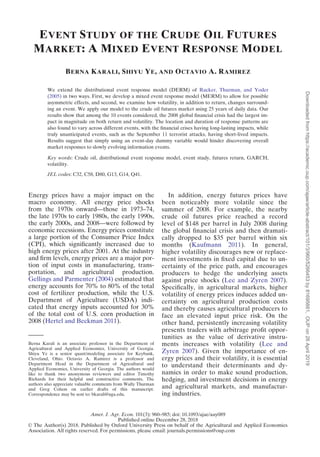
  • 5. lagged by one and two periods, respectively, k is the number of events, di t is a counter variable indicating the difference (in trading days) be- tween any given trading day t and the day event i occurred, et is the regression error term, and zt is a random variable that follows Student’s t distribution with degrees of free- dom. The count variable di t is zero on the event day; it takes negative values before and positive values after the event day. The term ht is the conditional variance representing our measure of volatility, and htÀ1 is the conditional variance lagged by one period. The explanatory variable fR i di t; hR i Þ À in the return equation is a probabil- ity density function evaluated at di t with param- eter vector hR i . Rucker, Thurman, and Yoder (2005) find, in their analysis, statistical similar- ity of the models when the density functions of their three types of events are specified as ei- ther a uniform or a normal distribution. Therefore, we specify the density function for seven of the ten events as a normal probability density function. However, for the three events that were most likely complete surprises to market participants (the September 11 terrorist attacks, Hurricane Katrina, and Iraq’s invasion of Kuwait denoted as Iraq1), and thereby might have led to asymmetric return and variance responses, we specify the density function as a type II generalized extreme value density function: ð2Þ fR i ðdi t; hR i Þ ¼ 1 rR i exp À 1 þ nR i di t À lR i À Á rR i !À 1 nR i 0 B B @ 1 C C A  1 þ nR i di t À lR i À Á rR i !À1À 1 nR i for September 11; Katrina; and Iraq1; 1 rR i ffiffiffiffiffiffi 2p p exp À di t À lR i À Á2 2rR2 i ! other events: 8 : Under this assumption, the DERM becomes a mixed event response model, which we de- note as MERM. While we assume a normal density function for seven events, the values of its parameters (location lR i and dispersion rR i ) are allowed to vary for each of these seven events. Similarly, the parameters of generalized extreme value density function Excess returns 1 ∗ β1 1 1 1 β3 3 3 3 3 1 t2 t2 * t1 t1 * t3 t3 * Day β2 2 2 2 0 Figure 1. The mixed event response model Note: Days t1, t2, and t3 denote the event days, and days tà 1, tà 2, and tà 3 denote the peak days corresponding to the mode of the underlying density function. For the first and second events, a normal density function is plotted, where mode¼l. For the third event, a type II generalized extreme value density function is plotted with n0, where mode¼lþ(r/n)((1þ n )-n –1). 964 April 2019 Amer. J. Agr. Econ. Downloadedfromhttps://academic.oup.com/ajae/article-abstract/101/3/960/5266453by81695661,OUPon26April2019
  • 6. (location lR i , dispersion rR i , and shape nR i ) are allowed to differ for the three events, that is, September 11, Katrina, and Iraq1. The ex- planatory variable fV i di t; hV i Þ À in the condi- tional variance equation has the same formula with fR i di t; hR i Þ À but includes differ- ent distributional parameters in hV i (i.e., loca- tion lV i , dispersion rV i , and shape nV i ) for a given density function to allow event impacts on volatility to vary from the event responses in return.3 Figure 1 modifies figure 2 in Rucker, Thurman, and Yoder (2005) to illustrate the MERM. Consider three different events that occurred on days t1, t2, and t3, with the first two events having a normal density response pattern and the third event having an asym- metric response pattern such as a type II Table 1. Event Descriptions Event Date Description Event Group (1) September 11 9/17/2001 The September 11 terrorist attacks led to an immediate halt on trading in all major trading markets until September 17th. The World Trade Center was destroyed, the Pentagon was heavily damaged, thousands of people were killed, and aviation was paused in the United States. Katrina 8/29/2005 Hurricane Katrina formed on August 23rd in the Bahamas and hit the U.S. Gulf coast on August 29th. This hurricane was the costliest natural disaster in the U.S. history, damaging 30 oil platforms and forcing nine refineries to close down for about six months. Event Group (2) Iraq1 8/02/1990 Iraq invaded Kuwait with one of the motivations being to prevent Kuwait from over-producing oil. Iraq2 1/17/1991 The U.S. military forces intervened in the Gulf War starting in the evening of January 16th in response to Iraq’s invasion of Kuwait. Iraq3 3/20/2003 The U.S. invaded Iraq, a carryover from the war in Afghanistan which started in response to the September 11 terrorist attacks. Event Group (3) OPEC1 8/27/1990 OPEC members announced a production-raise plan to help meet the supply shortfall caused by Iraq’s invasion of Kuwait on August 2, 1990. OPEC2 3/23/1999 OPEC announced a production-cut decision for one year made during the Organization’s 107th meeting in Vienna, effective starting April 1, 1999. OPEC3 12/17/2008 OPEC announced a production-cut decision, the largest ever announced, made during the 151st meeting in Algeria. Event Group (4) Asian financial crisis 7/02/1997 The Asian financial crisis started in Thailand with the financial collapse of the Thai baht, spread to many developing countries thereafter, and lasted from July 1997 to February 1998. Global financial crisis 9/15/2008 Lehman Brothers’ announced its filing for bankruptcy. The announcement was taken as a clear indicator of the evolving global 2007–2008 financial crisis. Note: Event dates are adjusted for time zone differences, weekends, holidays, and trading hours. 3 The model is also estimated with the density function of each event in return and variance equations specified as a normal distribution, which is denoted as the Normal Event Response Model (NERM) by Rucker, Thurman, and Yoder (2005). However, the Vuong test (1989), which indicates whether one model fits the data better than the other, rejects the equality of the two non-nested models in favor of the MERM at the 1% level. When the model is estimated with all density functions specified as a Johnson’s SU distribution to allow for more flexibil- ity through a wide range of skewness and kurtosis compared to a normal distribution, the Vuong test fails to reject the equality of that model to the NERM at the 10% level. Karali, Ye, and Ramirez Event Study of the Crude Oil Futures Market: A Mixed Event Response Model 965 Downloadedfromhttps://academic.oup.com/ajae/article-abstract/101/3/960/5266453by81695661,OUPon26April2019
  • 7. generalized extreme value density function. The distributional parameters, li, ri for i ¼ 1; 2; 3, and ni for i ¼ 3, determine the lo- cation, dispersion, and shape of the response patterns for each event. Specifically, the mode of the associated distribution, repre- sented by tà i in the figure, corresponds to the day on which the event response peaks. The mode is equal to the parameter li for normal density functions and to li þ ðri=niÞ ð 1 þ nið ÞÀni À 1Þ for the generalized extreme value function. Besides the distributional parameters, each event has its own scaling parameter, bi, which allows for a different magnitude and sign of each event’s effect. From the figure, for instance, it can be seen that the second event has a negative effect and its magnitude is about two-thirds the size of the first event’s effect. Since probabil- ities are measured over intervals, not single points, for continuous density functions, the area under the curve between two distinct points defines the probability for that inter- val. When that area under the density func- tion is multiplied by the scaling parameter bi, it shows the impact of the event on the Figure 2. Crude oil futures, 1990–2014 966 April 2019 Amer. J. Agr. Econ. Downloadedfromhttps://academic.oup.com/ajae/article-abstract/101/3/960/5266453by81695661,OUPon26April2019
  • 8. returns within a window. For instance, around day t1, the impact of the first event on the daily return is the shaded area under the curve surrounding t1, which is simply denoted as Rt1 . As time goes by, the impact of this event increases until day tà 1, and then starts to diminish. Because the MERM is a nonlinear model, estimation through OLS is not feasible. Once the trading day counter variable, di t, is plugged into the density functions given in equation (2), the parameters of the densities can be estimated along with the other model parameters using the maximum likelihood method. As previously indicated, our likeli- hood function is based on a regression error term, et in equation (1), following Student’s t distribution rather than a normal distribution, which is a separate issue from the event re- sponse patterns modelled as having a normal or a generalized extreme value probability density function. Data Event Descriptions Many events have the potential to impact crude oil futures prices. While some events could be a complete surprise, meaning that they are almost impossible to predict, others could have been predicted in advance based on the preceding stages. In addition, events could differ by the duration of their potential impact in unfolding and affecting the market. It could be that the full implications of the event cannot be ascertained for a long period of time, or the duration and eventual severity of the event itself are unpredictable. Even though numerous events could potentially af- fect energy prices, we focus on a total of ten events, a mix of geopolitical, economic, and weather-related events that have been shown to be moving crude oil prices in previous studies (Ye, Zyren, and Shore 2002; Olowe 2010; Hamilton 2011; Schmidbauer and Rosch 2012; Karali and Ramirez 2014; EIA 2015). Our study categorizes the included ten events into four groups based on their nature and potential duration: (1) weather-related or terrorist attack events; (2) invasions or wars related to the Middle East; (3) OPEC’s pro- duction change events; and (4) financial cri- ses.4 Table 1 provides the list of included events in each group. We briefly describe these events below and elaborate on their implications on crude oil markets when we discuss the empirical results. Figure 2. Continued 4 We should reemphasize that we estimate a distinct response pattern for each event, both in return and variance equations, and that we categorize the events into four groups only for moti- vating our expectations about their implications on the crude oil market and for discussing the results. Karali, Ye, and Ramirez Event Study of the Crude Oil Futures Market: A Mixed Event Response Model 967 Downloadedfromhttps://academic.oup.com/ajae/article-abstract/101/3/960/5266453by81695661,OUPon26April2019
  • 9. Event Group (1). In this group, we include the September 11 terrorist attacks and Hurricane Katrina. The attacks happened on Tuesday, September 11, 2001; trading stopped immediately after and started back on September 17, 2001. Hurricane Katrina formed on August 23, 2005 in the Bahamas and hit the U.S. Gulf coast on August 29, 2005. The variables dSep11 t and dKatrina t are cre- ated to count the trading days between any given day in our sample period and the event days of September 17, 2001 and August 29, 2005, respectively. Both the terrorist attacks and the forma- tion, not the landfall, of Hurricane Katrina were not anticipated and were considered to be “contained” in the sense that their impacts on the crude oil markets were straightforward to ascertain (disruption in either energy de- mand or supply). Therefore, even though they might have had extensive and lingering effects on the economy, we expect that they were fully processed and internalized by crude oil market participants in a relatively short period of time. Furthermore, due to their quite unexpected nature, especially for the terrorist attacks, we model the market re- sponse to these events as having the shape of a type II generalized extreme value probabil- ity density function that allows for asymmet- ric effects. Event Group (2). We include the three military invasions that involved Iraq during our sample period in this event group. The first event is Iraq’s invasion of Kuwait on August 2, 1990. The second event is the direct intervention by the United States on the eve- ning of January 16, 1991 in response to Iraq’s invasion of Kuwait. The third is the U.S. inva- sion of Iraq on March 20, 2003, a carryover from the war in Afghanistan that started in response to the September 11 terrorist attacks. The variables dIraq1 t , dIraq2 t , and dIraq3 t are created to count the trading days between any given day and the event days of August 2, 1990, January 17, 1991, and March 20, 2003, respectively. Since the implications of these wars on crude oil were readily apparent (disruption in oil supply), we expect that it took a short period of time for the information to be fully processed and internalized by the market participants. In addition, despite the tension between Iraq and Kuwait be- fore the invasion, the invasion itself was not expected and took Kuwait and most Arab parties by surprise (Kostiner 2009). On the other hand, there was a buildup be- fore the second and third Iraq events, and therefore the events were somewhat antici- pated. Accordingly, we specify the proba- bility density function for the response pattern as a type II generalized extreme value distribution for the Iraq1 event, and as a normal distribution for the Iraq2 and Iraq3 events. Event Group (3). Three production change decisions by OPEC are included in this event group. The first OPEC event on August 27, 1990 was the announcement of a production- raise plan, and was therefore expected to re- sult in a decrease in prices, while the other two events on March 23, 1999 and December 17, 2008 were production-cut announcements bringing about an increase in prices. The vari- ables dOPEC1 t , dOPEC2 t , and dOPEC3 t are created to count the trading days between any given day and the event days August 27, 1990, March 23, 1999, and December 17, 2008, respectively. In theory, the movement of crude oil prices after OPEC’s production change decisions should be a straightforward result of supply and demand interactions. However, since OPEC had problems in maintaining and enforcing production quotas among member countries (Williams 2011), we expect the du- ration of these events to be long-lasting in the sense that it took a prolonged time period for the market price to adjust to its new equilib- rium level. Event Group (4). In this event group, we include the Asian financial crisis that started in Thailand and lasted from July 1997 to February 1998. The second event is the 2007– 2008 financial crisis. While there was no spe- cific event marking the beginning of this cri- sis, Lehman Brothers’ announcement of its filing for bankruptcy on September 15, 2008 was taken as a clear indicator of the evolving global crisis. The variables dAsian t and dGlobal t are created to compute the differences be- tween any trading day in our sample and the event days of July 2, 1997 and September 15, 2008, respectively. Since financial crises can be related to previous economic phenomena (e.g., high default rate in the subprime home mortgage before the global financial crisis) and resuming the economic growth after- wards might be lengthy (Hamilton 2011), we expect their impacts to be fully internalized over a long period of time. 968 April 2019 Amer. J. Agr. Econ. Downloadedfromhttps://academic.oup.com/ajae/article-abstract/101/3/960/5266453by81695661,OUPon26April2019
  • 10. Futures Returns We study crude oil futures contracts that are traded at the CME Group from April 1990 to December 2014. The Light Sweet Crude Oil (WTI) futures contracts play an important role in managing risk in the energy sector worldwide because they are the most liquid energy hedging vehicles (CME 2014). These contracts have expiration dates in every month of the year and are traded until the third business day prior to the 25th calendar day of the month preceding the delivery month. We construct a single price series by rolling over the first nearby contract on the 15th day of the expiration month (the month preceding the contract month). The daily return on a futures contract is de- fined as Rt ¼ 100 Â lnPt À lnPtÀ1ð Þ, where Pt is the closing price of the nearby contract on trading day t. Descriptive statistics of the re- turn and absolute return on crude oil futures contracts are summarized in table 2.5 There are 6,194 observations in the sample. The av- erage return is 0.016% with a standard devia- tion of 2.158%. The average daily absolute return, Rtj j, on the other hand, is 1.522%, with a standard deviation of 1.529%. According to the Kolmogorov-Smirnov and Jarque-Bera tests, the returns are not nor- mally distributed and exhibit significant left skewness and excess kurtosis. Figure 2 shows the daily futures price, return, and absolute return series for the entire sample period. One can see a dramatic increase in the crude oil price in 2008, followed by a remarkable drop, with an obvious volatility clustering during the Gulf War, after the September 11 terrorist attacks, and after OPEC’s produc- tion cut in 2008. Results Table 3 reports the results from the MERM estimation. The estimated degrees of free- dom, , is 7.898 and statistically significant at the 1% level. The intercept and the coeffi- cients of the autoregressive terms in the re- turn equation are statistically insignificant at the 10% level. While the finding of the insig- nificant intercept is in line with the average daily return of 0.016% shown in table 2 with a standard deviation of 2.158%, yielding a t- value of 0.007 and thereby indicating statisti- cal insignificance, the lack of negative serial correlation in returns is inconsistent with the findings of Bu (2014) and Schmidbauer and Rosch (2012) but consistent with the Martingale model, which assumes that price changes are unpredictable (Theodossiou and Lee 1995). In addition, the significance of the ARCH and GARCH terms confirms that us- ing a GARCH model is appropriate in this case. The likelihood ratio (LR) test for the exclusion of the density functions in both re- turn and variance equations in equation (1) is rejected at the 1% level. Tables 4 and 5 present the magnitude and duration of event impacts on crude oil return and variance, respectively, based on the esti- mated density function parameters provided in table 3. The magnitudes of event impacts are shown in three ways. Overall impact repre- sents the total area under the density function (i.e., one) multiplied by the scaling factor b. Impact magnitudes within an event window are computed as bPr(t À z dt t þ z), reflecting the area under the density function over the interval [t À z, t þ z] multiplied by the scaling factor b, where t is either the event Table 2. Summary Statistics of Crude Oil Futures Return and Absolute Return Return Absolute Return Mean 0.016 1.522 Median 0.066 1.114 Standard Deviation 2.158 1.529 Maximum 13.340 38.407 Minimum À38.407 0.000 Skewness À1.168 4.314 (0.001) (0.001) Excess Kurtosis 22.634 65.438 (0.001) (0.001) Kolmogorov-Smirnov 0.129 0.500 (0.001) (0.001) Jarque-Bera 100,900 1,025,400 (0.001) (0.001) No. of Observations 6,194 6,194 Note: Values in parentheses are two sided p-values for the skewness and kurtosis tests, and one-sided p-values for the Kolmogorov-Smirnov and Jarque-Bera normality tests. 5 Absolute return is a commonly used proxy for volatility. It should be noted that we present the descriptive statistics and a graph of absolute return only to provide the readers a sense of volatility in the crude oil market. We measure the volatility dy- namics in the crude oil market through the GARCH specification outlined above, which allows for time-varying conditional vari- ance and simultaneous estimation of the model parameters in both return and variance equations. Karali, Ye, and Ramirez Event Study of the Crude Oil Futures Market: A Mixed Event Response Model 969 Downloadedfromhttps://academic.oup.com/ajae/article-abstract/101/3/960/5266453by81695661,OUPon26April2019
  • 11. Table3.MixedEventResponseModelResultsforCrudeOilFuturesMarket ReturnVariance bR lR rR nR bV lV rV nV EventGroup(1) September11À29.4855.1570.121§ 0.2016.124À2.2360.7590.202 (3.712)(0.121)(0.085)(0.068)(0.565)(0.188)(0.079)(0.069) Katrina6.057À2.8480.1100.2071.404À0.9430.2340.247 (0.460)(0.089)(0.044)(0.096)(0.127)(0.132)(0.044)(0.041) EventGroup(2) Iraq134.9970.8372.7890.3151.7782.9590.049§ 0.291§ (5.508)(0.480)(0.427)(0.113)(0.416)(0.195)(0.075)(0.409) Iraq2À91.1390.4090.251§ À7.0073.9860.203 (3.335)(0.109)(0.167)(1.954)(0.299)(0.058) Iraq3À30.216À2.1182.1395.162À2.9732.381 (1.877)(0.238)(0.274)(0.268)(0.354)(0.137) EventGroup(3) OPEC1À25.044À0.3830.28312.3721.7240.263§ (3.180)(0.105)(0.091)(1.961)(0.289)(0.313) OPEC241.571À4.16013.467À1.071À9.96318.127 (3.133)(0.326)(0.805)(0.188)(0.561)(0.789) OPEC332.980103.21410.268À12.43775.5522.421 (0.638)(3.584)(0.394)(0.409)(1.293)(0.126) EventGroup(4) AsianfinancialcrisisÀ92.51199.99599.984À0.57985.0000.213§ (3.357)(7.820)(4.191)(0.213)(4.831)(0.175) GlobalfinancialcrisisÀ166.76133.08538.99941.87015.22317.355 (2.925)(1.491)(0.921)(1.349)(0.593)(0.438) Intercept(a)(x)0.057§ 0.012 (0.043)(0.004) Returnlag1(b1)À0.024§ (0.019) Returnlag2(b2)À0.022§ (0.015) ARCH(a)0.034 (0.011) GARCH(c)0.963 (0.012) DegreesofFreedom()7.898 (0.114) LLFÀ12,505.290 AIC25,156.580 BIC25,647.968 LRtest209.127 [0.001] Note:ThemodelisRt¼aþb1RtÀ1b2RtÀ2þ Pk i¼1bR ifR idi t;hR iÞþet; À withet¼zt ffiffiffiffiffi ht p andht¼xþae2 tÀ1þchtÀ1þ Pk i¼1bV ifV idi t;hV iÞ; À wherefR iÁðÞandfV iÁðÞindicateeithernormalortypeIIgeneralizedextremevaluedensityfunction. Standarderrorsareshowninparentheses.Thesymbol§denotesstatisticalinsignificanceatthe10%level.Thenullhypothesisofthelikelihoodratio(LR)testisjointexclusionofeventimpactsinbothreturnandvarianceequations,andits p-valueisshowninsquarebrackets.LLF,AIC,andBICrefer,respectively,tolog-likelihoodfunction,Akaike,andBayesianinformationcriteria. 970 April 2019 Amer. J. Agr. Econ. Downloadedfromhttps://academic.oup.com/ajae/article-abstract/101/3/960/5266453by81695661,OUPon26April2019
  • 12. day or peak day; z ¼ 0.3 for events with dura- tion less than five trading days, and z ¼ 3 oth- erwise.6 For duration of event impacts, the start and end days are computed as the 5th and 95th percentiles of the associated event’s distribution, and peak days are calculated as the estimated mode of each distribution. Duration (in trading days) is then calculated as the difference between the 95th and 5th percentiles to reflect the length of event impacts for 90% of the observations. The tables also present (in parentheses) the associ- ated dates that are determined after simple rounding of the estimated peak, and the 5th and 95th percentiles. In addition, the esti- mated event response patterns in the daily returns and variances are depicted in figures 3 through 6. In the following pages, we will walk readers through the implications of these esti- mates and findings. Event Group (1) The September 11 terrorist attacks led to an immediate halt on trading. As a result of the attacks, the World Trade Center was destroyed, the Pentagon was heavily dam- aged, and thousands of people were killed. Aviation was paused in the United States, and all major trading markets (including en- ergy) were closed for the remainder of the week. The economic damage from these attacks was estimated to be in the billions. Markets reopened a week later, and futures prices of crude oil and petroleum products fell to their lowest levels in nearly two years, presumably due to fears that a recession would reduce energy demand.7 Table 4 suggests that the attacks led to an overall drop of 29.485 percentage points in crude oil futures return. In fact, a major por- tion of the decline, as much as 25.332 per- centage points, occurred during the event window of [þ4.835, þ5.435], which is 0.3 trad- ing days around the peak day of 5.135. The estimated duration of the return response is about one trading day, surrounding September 24, 2001, the fifth trading day after the markets reopened on September 17th (i.e., our event day).8 Table 5 shows that the variance response is estimated to peak two trading days before the event. The variance response was an increase of 0.276 during the event-day window and an increase of 1.756 during the peak-day window. The pre-event variance peak is somewhat odd given the complete surprise nature of the attacks, sug- gesting that there might have been an unre- lated blip in the crude oil futures market. The estimates from our model show that the im- pact of this event was short-lived in the crude oil futures market, especially for the return, and did not trigger a long-term trend of de- creasing oil prices (figure 3). The relationship between return and variance appears to be negative, and the variance response seems to lead the return response. Hurricane Katrina started as a tropical de- pression that formed on August 23, 2005 in the Bahamas and became a tropical storm during the following day. The storm moved through the northwestern Bahamas on August 24-25 and then turned toward south- ern Florida. It became a hurricane just before making landfall near the Miami-Dade/ Broward county line during the evening of August 25. The hurricane then moved across southern Florida into the eastern Gulf of Mexico on August 26, strengthening signifi- cantly and reaching Category 5 intensity on August 28. The hurricane turned to the north, with the center making landfall near Buras, Louisiana, on August 29, 2005. Continuing northward, the hurricane made a second landfall near the Louisiana/Mississippi border on the same day. The cyclone weakened to a tropical depression over Tennessee Valley on August 30. Katrina became an extratropical low on August 31, 2005. This hurricane was the costliest natural disaster, as well as one of the five deadliest hurricanes, in U.S. history. Katrina damaged or destroyed 30 oil plat- forms. In addition, nine refineries were forced 6 While the choice of 0.3 and 3 days for event windows is arbi- trary, as well as the duration of five days, it helps us to demon- strate the magnitude of event impacts surrounding the event day and the peak day. 7 The September 11 terrorist attacks aggravated the 2001 re- cession, which had begun in March 2001 and ended in November 2001. Kliesen (2003) shows that while only 13% of Blue Chip forecasters believed that the U.S. economy had slipped into a re- cession as of September 10, 2001, the percentage increased to 82% as of September 19, 2001. 8 Even though the U.S. stock market experienced a sharp de- cline (7.1% decrease in the Dow Jones Industrial Average index) on the day trading recommenced, the decrease in the crude oil price was more gradual. The spot price was $27.66 per barrel on September 10th, $27.65 on September 11th, the day of the attacks, and $27.64 on September 12th. The spot price increased to $28.84 on September 17th and started to fall afterwards, reach- ing to $21.46 on September 24th, after which it started to in- crease. Similarly, the futures price was $27.85 per barrel on September 10th, increased to $29.17 on September 17th, de- creased each consecutive day, and reached $22.01 on September 24th. Karali, Ye, and Ramirez Event Study of the Crude Oil Futures Market: A Mixed Event Response Model 971 Downloadedfromhttps://academic.oup.com/ajae/article-abstract/101/3/960/5266453by81695661,OUPon26April2019
  • 13. Table4.EventImpactsonCrudeOilFuturesReturn EstimatedMagnitudeofEventImpacts(p.p.)EstimatedDurationofEventImpacts(tradingdays) OverallEventday6zPeakday6zDurationEventdayStartday[5th pctl]PeakdayEndday[95th pctl] EventGroup(1) September11À29.4850.000À25.3320.61205.0385.1355.650 (9/17/2001)(9/24/2001)(9/24/2001)(9/25/2001) Katrina6.0570.0015.3260.5570À2.956À2.868À2.399 (8/29/2005)(8/24/2005)(8/24/2005)(8/25/2005) EventGroup(2) Iraq134.99721.15421.43416.3050À1.7510.10614.553 (8/02/1990)(7/31/1990)(8/02/1990)(8/24/1990) Iraq2À91.139À30.018À69.9240.8270À0.0040.4090.823 (1/17/1991)(1/17/1991)(1/17/1991)(1/18/1991) Iraq3À30.216À19.687À25.3587.0390À5.638À2.1181.401 (3/20/2003)(3/12/2003)(3/18/2003)(3/21/2003) EventGroup(3) OPEC1À25.044À9.434À17.8010.9320À0.849À0.3830.083 (8/27/1990)(8/24/1990)(8/27/1990)(8/27/1990) OPEC241.5716.9927.32844.3010À26.312À4.16017.989 (3/23/1999)(2/12/1999)(3/17/1999)(4/19/1999) OPEC332.9800.0007.58033.765086.326103.214120.091 (12/17/2008)(4/23/2009)(5/18/2009)(6/11/2009) EventGroup(4) AsianfinancialcrisisÀ92.511À1.343À2.214328.9190À64.49199.995264.428 (7/02/1997)(4/02/1997)(11/21/1997)(7/22/1998) GlobalfinancialcrisisÀ166.761À7.140À10.225128.2620À31.04433.08597.218 (9/15/2008)(7/31/2008)(10/30/2008)(2/03/2009) Note:Eventimpactmagnitudes(inpercentagepoints)arecomputedasbR PrðtÀzdttþzÞwheret¼eventdayorpeakday,z¼0.3foreventswithadurationoflessthan5tradingdays,andz¼3otherwise.Overallmagnitudesarepre- sentedasbR .Thestartandenddaysarecomputedasthe5thand95thpercentilesoftheassociatedevent’sdistribution,andpeakdaysarecalculatedastheestimatedmodeofeachdistribution.Duration(intradingdays)iscalculatedasthe differencebetweenthe95thand5thpercentilestoreflectthelengthofeventimpactsfor90%oftheobservations.Thedatesgiveninparenthesesaredeterminedaftersimpleroundingoftheestimatedpeak,andthe5thand95thpercentiles. 972 April 2019 Amer. J. Agr. Econ. Downloadedfromhttps://academic.oup.com/ajae/article-abstract/101/3/960/5266453by81695661,OUPon26April2019
  • 14. Table5.EventImpactsonCrudeOilFuturesVariance EstimatedMagnitudeofEventImpactsEstimatedDurationofEventImpacts(tradingdays) OverallEventday6zPeakday6zDurationEventdayStartday[5th pctl]PeakdayEndday[95th pctl] EventGroup(1) September116.1240.2761.7563.8330À2.983À2.3730.850 (9/17/2001)(9/06/2001)(9/07/2001)(9/18/2001) Katrina1.4040.1160.9511.2510À1.168À0.9930.083 (8/29/2005)(8/26/2005)(8/26/2005)(8/29/2005) EventGroup(2) Iraq11.7780.0001.7220.27502.9142.9473.188 (8/02/1990)(8/07/1990)(8/07/1990)(8/07/1990) Iraq2À7.0070.000À6.0360.66603.6533.9864.319 (1/17/1991)(1/23/1991)(1/23/1991)(1/23/1991) Iraq35.1622.5734.0907.8350À6.893À2.9730.943 (3/20/2003)(3/11/2003)(3/17/2003)(3/21/2003) EventGroup(3) OPEC112.3720.0009.2340.86501.2921.7242.156 (8/27/1990)(8/28/1990)(8/29/1990)(8/29/1990) OPEC2À1.071À0.121À0.14159.6050À39.754À9.96319.851 (3/23/1999)(1/25/1999)(3/09/1999)(4/21/1999) OPEC3À12.4370.000À9.7607.970071.56575.55279.535 (12/17/2008)(4/02/2009)(4/08/2009)(4/14/2009) EventGroup(4) AsianfinancialcrisisÀ0.5790.000À0.4870.700084.65085.00085.350 (7/02/1997)(10/31/1997)(10/31/1997)(10/31/1997) Globalfinancialcrisis41.8703.9265.74657.0560À13.29815.22343.758 (9/15/2008)(8/26/2008)(10/06/2008)(11/14/2008) Note:EventimpactmagnitudesarecomputedasbV PrðtÀzdttþzÞwheret¼eventdayorpeakday,z¼0.3foreventswithadurationoflessthan5tradingdays,andz¼3otherwise.OverallmagnitudesarepresentedasbV .Thestart andenddaysarecomputedasthe5thand95thpercentilesoftheassociatedevent’sdistribution,andpeakdaysarecalculatedastheestimatedmodeofeachdistribution.Duration(intradingdays)iscalculatedasthedifferencebetweenthe 95thand5thpercentilestoreflectthelengthofeventimpactsfor90%oftheobservations.Thedatesgiveninparenthesesaredeterminedaftersimpleroundingoftheestimatedpeak,andthe5thand95thpercentiles. Karali, Ye, and Ramirez Event Study of the Crude Oil Futures Market: A Mixed Event Response Model 973 Downloadedfromhttps://academic.oup.com/ajae/article-abstract/101/3/960/5266453by81695661,OUPon26April2019
  • 15. to close down for about six months and 24% of the annual oil production in the Gulf coast was lost. Consistent with the timeline of the hurri- cane’s formation, the duration of Katrina’s impact on crude oil is estimated to have lasted about a half trading day for returns (table 4), indicating that this weather event did not have a long-term effect on crude oil prices either. Furthermore, the peak-day win- dow impact of Hurricane Katrina was an in- crease of 5.326 percentage points in return (table 4) and 0.951 in variance (table 5). Given the relatively smaller magnitude and shorter duration of its influence, the model does not provide evidence that Hurricane Katrina was a substantial event in the crude oil futures market. Because the event day is chosen as the day the hurricane struck the Gulf coast on Monday, August 29th, the re- turn response peak-day estimate of À2.868 indicates that the peak impact was about three trading days before the event day, which is the day the storm started moving -2 0 2 4 6 Day 0 September 11 Return Variance Peak: -2.37 Peak: 5.14 -3.5 -3 -2.5 -2 -1.5 -1 -0.5 0 0.5 Day 0 Katrina Return VariancePeak: -2.87 Peak: -0.99 Figure 3. Crude oil futures market response to September 11 terrorist attacks (September 17, 2001) and Hurricane Katrina (August 29, 2005) Note: Response shapes are plotted as bR fR dt; hR Þ À for return, and as bV fR dt ; hV Þ À for variance. Peak refers to the estimated mode of each distribution and is shown relative to the event day. 974 April 2019 Amer. J. Agr. Econ. Downloadedfromhttps://academic.oup.com/ajae/article-abstract/101/3/960/5266453by81695661,OUPon26April2019
  • 16. through the Bahamas toward Florida. No re- turn impact is found on the event-day window as the landfall was expected a few days before. While Hurricane Katrina was the costliest hurricane at the time and had a long-term economic impact overall, our finding of shorter duration of its impact on crude oil futures return and variance could be explained by two factors. First, due to the dis- ruptions in oil production in the Gulf of Mexico, which accounted for 25% of domestic production, President George W. Bush autho- rized and directed the Secretary of Energy on September 2, 2005 to drawdown and sell crude oil from the Strategic Petroleum Reserve (SPR). On September 6, 2005, the Department of Energy issued a Notice of Sale, offering 30 million barrels of crude oil (Department of Energy 2018). However, be- cause the SPR, pipelines, and refineries were all affected by the hurricane, the release of unfinished crude oil into the market had lit- tle impact on prices (Boutwell 2012). The price of crude oil averaged at $64 per barrel in the weeks leading up to Hurricane Katrina, reached $67 per barrel when Katrina made landfall, fell to just under $66 per barrel when the sale was announced, and averaged $62 per barrel by October (Boutwell 2012). Second, in a press release by the U.S. Department of the Interior on October 4, 2005, it was stated that a large portion of the destroyed platforms were “end-of-life” facilities and accounted for only 1.7% of the Gulf’s oil production, and therefore only a small percentage of the pro- duction was expected to be permanently lost (U.S. Department of the Interior 2005). Event Group (2) Two of the three invasions involving Iraq were related to the first Gulf War.9 The first event occurred on August 2, 1990, when Iraq invaded Kuwait. The underlying factors be- hind the Iraq-Kuwait dispute, which esca- lated during the spring of 1990, included Iraq’s requests to reduce Kuwait’s oil produc- tion and write off Iraq’s debt. In fact, OPEC announced on July 25, 1990, a few days before the Iraq’s invasion, an agreement be- tween Kuwait and the United Arab Emirates to limit daily oil output to 1.5 million barrels, with the potential of settling Iraq’s concerns on lower oil prices due to Kuwait’s overpro- duction. At the time of this announcement though, Iraq had already deployed more than 100,000 troops along the Iraq-Kuwait border. Despite the increased tension, the invasion caught Kuwait off guard. Kostiner (2009) argues that Kuwait was strategically surprised because Kuwait believed that Iraq preferred economic development over a costly war, its strategy of neutrality between Iraq and Iran was effective, and its reliance on negotiations with Iraq, Arab states’ mediation, and ab- stention from military preparations would avoid war and invasion. After the invasion, oil production was expected to decline sharply, and prices increased accordingly be- cause one of the motivations for the invasion was to prevent Kuwait from over-producing oil. Table 4 suggests that the returns in- creased by 35 percentage points overall, argu- ably because the market expected Kuwait’s oil production to fall.10 The return response peaked on the day of the event, with a 21 per- centage point increase during the event/peak- day window, and lasted for about 16 trading days starting from July 31, 1990 (table 4). The impact on the variance, which peaked on the third trading day after the event, is measured as 1.722 during the peak-day window (table 5). It is also found that the duration of the variance response is shorter compared to the return response (figure 4). This suggests that the uncertainty about the implications of the invasion might have been resolved quickly. Hamilton (2011) explains the short- lived price spike as a result of Saudis using the substantial excess capacity they had been maintaining throughout the decade. The second event is the direct military in- tervention by U.S.-led forces in the Gulf War, starting on the evening of January 16, 1991, in response to Iraq’s invasion of Kuwait. The spot price of crude oil in Cushing, Oklahoma, fell by $10.77 per barrel (U.S. Energy Information Administration 2018) in response to the U.S. decision to re- lease stockpiles of crude from its massive SPR to compensate for any supply shortfalls9 The Gulf War (August 2, 1990–February 28, 1991), code- named Operation Desert Shield (August 2, 1990–January 17, 1991) for operations leading to the buildup of troops and defense of Saudi Arabia and Operation Desert Storm (January 17, 1991– February 28, 1991) in its combat phase, was a war waged by coali- tion forces from 34 nations led by the United States against Iraq in response to Iraq’s invasion and annexation of Kuwait. 10 Oil price shock is documented as a 93% increase in Hamilton (2011) from August to October 1990, and as a 53% in- crease in Economou (2016) for the same time period. Karali, Ye, and Ramirez Event Study of the Crude Oil Futures Market: A Mixed Event Response Model 975 Downloadedfromhttps://academic.oup.com/ajae/article-abstract/101/3/960/5266453by81695661,OUPon26April2019
  • 17. during the war. With the increasing world oil supply, prices continued to fall until 1994. Our results indicate that this event resulted in an overall return decrease of 91.139 percent- age points, 69.924 percentage points of which were observed within the peak-day window (table 4). However, the impact on returns lasted for only about one trading day (table 4 and figure 4). It should be noted that while the impact on returns might not be pro- longed, the impact on the price levels could be permanent, such that they have stayed at lower levels than before the invasion for a long time. This event also resulted in a vari- ance decrease of 6.036 around the peak day, which is estimated as about four trading days (table 5 and figure 4). It is not obvious why the return variance decreases following a de- crease in return. Given that the drop in the variance started after the event occurred, it could be argued that oil market participants fully internalized the implications of the war in the following few days and the uncertainty about future oil supply was therefore re- solved, reducing the return variance. Besides, this indicates a positive relationship between return and variance, which has been shown to exist in earlier work (French, Schwert, and Stambaugh 1987; Theodossiou and Lee 1995). The third event is the U.S. invasion of Iraq on March 20, 2003. This invasion was expected to stabilize global energy supplies as a whole by ensuring the free flow of Iraqi oil to the world markets (Muttitt 2012). Oil prices only decreased for a limited period of time, before resuming a long-term increasing trend. Our results show that this event brought about an overall return decrease of 30.216 percentage points and its impact lasted for about seven trading days (table 4). It also led to an increase of 5.162 in variance overall. Interestingly, the peak for both return and variance responses are found to occur two and three trading days, respectively, before the event, indicating that the third Iraq event was fully anticipated by the market partici- pants (figure 4). Event Group (3) The first supply-changing event by OPEC considered in our study occurred on August 27, 1990, when OPEC members gathered in- formally and announced their plan to raise oil production to help meet the supply shortfall caused by Iraq’s invasion of Kuwait on August 2, 1990. Since this event was the announcement of a production-raise plan, its expected impact was a decrease in returns. Our results suggest that the estimated impact duration of this event was only one trading day for both return and variance, and that the estimated overall impacts were -25.044 per- centage points and 12.372, respectively (tables 4 and 5). The finding of volatility increases are consistent with previous re- search focusing on OPEC meetings (e.g., Ye, Zyren, and Shore 2002; Lee and Zyren 2007; Karali and Ramirez 2014). The peak return response occurred right on the event day, and that of variance response on the second trad- ing day following the event (figure 5). The second OPEC event, which occurred on March 23, 1999, was a production-cut deci- sion made during the Organization’s 107th meeting in Vienna. In an effort to raise oil prices, which were at considerably low levels from late 1997 until early 1999, OPEC and non-OPEC countries agreed to cut oil output by a combined 2.104 million barrels (1.716 for OPEC members and 0.388 for non-OPEC members) per day. This pledge was for one year, effective April 1, 1999. Our results sug- gest that the overall impact on returns was 41.571 percentage points, and the duration of the return response was about 44 trading days (table 4). The variance response lasted for about 60 trading days, and the overall im- pact was a decrease of 1.071 (table 5). There is usually widespread speculation before OPEC meetings about what type of produc- tion decision will be announced (Schmidbauer and Rosch 2012). However, this production-cut decision was actually reached at The Hague meeting, a smaller group of key OPEC and non-OPEC players getting together ahead of the full meeting in order to solve important issues, which took place on March 11–12, 1999. The official OPEC meeting in Vienna on March 23rd merely formalized this understanding reached at The Hague (IEA 1999). We find that the return and variance responses consis- tently peaked about four and ten trading days before the event, respectively (figure 5). Our finding of the pre-event variance impact is also consistent with the findings in Schmidbauer and Rosch (2012). The third event occurred during OPEC’s 151st meeting in Oran, Algeria, on December 17, 2008. In addition to the output-cut agree- ments of 500,000 barrels a day made in September and of 1.5 million barrels a day made in October, the Organization 976 April 2019 Amer. J. Agr. Econ. Downloadedfromhttps://academic.oup.com/ajae/article-abstract/101/3/960/5266453by81695661,OUPon26April2019
  • 18. announced a decision to further cut produc- tion by 2.2 million barrels a day beginning in January 2009. This cut was the largest ever announced by OPEC, and therefore expected to cause oil prices to increase. However, this decision was widely anticipated by crude oil market participants; in fact, Saudi Arabia’s Oil Minister told reporters before the meet- ing that OPEC would cut 2 million barrels a day. Therefore, traders were unmoved with this production-cut decision, and the price of oil dropped to 4.5-year low after the an- nouncement (Musante 2008). In addition, this announcement was made during the global fi- nancial crisis that resulted in an economic downturn (Duggan 2016). Table 4 shows that the return increased overall by 32.980 percentage points, but the response peaked 103 trading days after the event. The overall variance impact was a decrease of 12.437 and, similar to the return response, was a delayed response, which peaked about 76 trading days after the event (table 5). The delayed responses to the third OPEC event seen in figure 5 can be explained by the following factors. After the production-cut announcement on December 17th, OPEC’s President also left the door open for more production cuts in the future if the markets were surprised with the current decision and stated that the member states were prepared to hold another meeting sooner than the scheduled March 15th meeting if needed (Musante 2008). Saudi Arabia’s Oil Minister -2 0 2 4 6 8 10 12 Day 0 Iraq1 Return VariancePeak: 2.95 Peak: 0.11 0 1 2 3 4 5 Day 0 Iraq2 Return Variance Peak: 3.99 Peak: 0.41 -10 -5 0 5 10 15 Day 0 Iraq3 Return VariancePeak: -2.97 Peak: -2.12 Figure 4. Crude oil futures market response to Iraq1 (August 2, 1990), Iraq2 (January 17, 1991), and Iraq3 (March 20, 2003) Note: Response shapes are plotted as bR fR dt; hR Þ À for return, and as bV fV dt; hV Þ À for variance. Peak refers to the estimated mode of each distribution and is shown relative to the event day. Karali, Ye, and Ramirez Event Study of the Crude Oil Futures Market: A Mixed Event Response Model 977 Downloadedfromhttps://academic.oup.com/ajae/article-abstract/101/3/960/5266453by81695661,OUPon26April2019
  • 19. said the Kingdom would go beyond its OPEC pledge, and market analysts expected the Kingdom to cut its production in February by an additional 300,000 barrels a day below its OPEC quota (Mouawad 2009). Even though there were signs by early January that OPEC members were complying with their pledge to limit oil supply, crude oil stocks at Cushing, Oklahoma (the WTI futures con- tract’s delivery point), were at an all-time high (IEA 2009a). As a result, the aggressive production cut did not affect the prices in the near term. Economou (2016), in fact, demon- strates that a negative flow supply shock (such as OPEC production cuts) causes a per- sistent and gradually increasing effect on the real price of oil that peaks after one year. These arguments explain the relatively slow adjustment in returns and variance predicted by our model. The movements in oil price are summarized in the Oil Market Reports that are published monthly by the International Energy Agency (IES). The reports reveal that crude oil price exceeded $50 per barrel for the first time in four months as more bull- ish sentiment entered financial markets in late March-early April, but weak market fun- damentals limited further gains (IEA 2009b); oil price strengthened to a six-month high by early May, but bullish macroeconomic senti- ment did not produce signs of oil demand re- covery (IEA 2009c); and the bull run was largely driven by perceived global economic recovery (IEA 2009d). In July, however, the crude oil price reached an eight-week low due to growing concerns about the economic recovery, persistently high oil stocks, and weak demand (IEA 2009e). -1 0 1 2 3 4 Day 0 OPEC1 Return Variance Peak: 1.72 Peak: -0.38 60 70 80 90 100 110 120 130 140 Day 0 OPEC3 Return Variance Peak: 103.2 Peak: 75.55 Figure 5. Crude oil futures market response to OPEC1 (August 27, 1990), OPEC2 (March 23, 1999), and OPEC3 (December 17, 2008) Note: Response shapes are plotted as bR fR dt ; hR Þ À for return, and as bV fV dt; hV Þ À for variance. Peak refers to the estimated mode of each distribution and is shown relative to the event day. 978 April 2019 Amer. J. Agr. Econ. Downloadedfromhttps://academic.oup.com/ajae/article-abstract/101/3/960/5266453by81695661,OUPon26April2019
  • 20. Event Group (4) The Asian financial crisis started in Thailand with the financial collapse of the Thai baht af- ter the Thai government was forced to float the baht. The crisis lasted from July 1997 to February 1998, and led to an economic slow- down in developing countries in many parts of the world and therefore to a large decrease in the demand for oil. This reduced the price of crude oil to as low as $10 per barrel, trig- gering an OPEC policy change to restore oil prices to higher levels. Due to the prolonged financial crisis, we expect its impact on the oil market to last for a long time. Table 4 shows a negative return response, in line with previous research (e.g., Olowe 2010; Ye, Zyren, and Shore 2002), amounting to an overall drop of 92.511 percentage points over a year. The return response peaked at about 100 trading days after the event, and the impact is estimated to last for 329 trading days. The variance response to this event was a 0.579 drop, which occurred 85 trading days after the event and lasted for only about one trading day. These delayed responses in both return and variance (figure 6) suggest that ad- ditional developments related to the Asian crisis, or some other event not included in our study, occurred in the following four to five months, affecting both the return and variance. However, it should also be noted that world petroleum consumption did not re- turn to strong growth until 1999; the pro- longed reduced demand led to the lowest oil price seen since 1972 by the end of 1998 (Hamilton 2011). Economou (2016), in fact, states that the oil price shock due to the Asian financial crisis as À57% for the period from December 1997 to December 1998. The filing of bankruptcy by Lehman Brothers, at that time one of the major invest- ment banks, on September 15, 2008 certainly precipitated the events that resulted in dimin- ishing credit lines in financial markets, creat- ing a credit constraint for firms and consumers. This was followed by a substantial decrease in the demand for crude oil, gasoline, and other energy commodities. Accordingly, the global financial crisis is found to affect the returns negatively and the variance positively. For the daily return, the largest impact is found 33 trading days after the event, with an overall impact of a 166.761 percentage-point drop between July 2008 and February 2009 (table 4). This finding is in line with the nega- tive price shock of 102% reported in Economou (2016) for a shorter time period, from July 2008 to December 2008. The daily return decreased by 7.140 percentage points within the event-day window of [À3, þ3] and by 10.225 percentage points within the peak- day window of [þ30, þ36]. The variance re- sponse was an overall increase of 41.870 from August 2008 to November 2008, with a 3.926 increase during the event-day window and a 5.746 increase during the peak-day window of [þ12, þ18]. Figure 6 shows the peak return re- sponse on the 33rd trading day after the event and the peak variance response on the 15th trading day. These findings are in contrast to previous research that suggested the 2008 fi- nancial crisis had no impact on oil returns and volatility (e.g., Olowe 2010; Karali and Ramirez 2014). However, those earlier studies do not allow for a flexible response pattern in return and variance, and employ a dummy variable approach instead. The impact duration of both financial crises on the returns is estimated to be over 100 trading days, which is considerably longer than all the other eight events. This suggests, consistent with our expectations, that financial crises consist of multiple events and the total- ity of this information does not occur and/or is hard to absorb in a short period of time. Discussion The finding of delayed and prolonged responses to some of the events (specifically the Asian and global financial crises and OPEC’s meetings in March 1999 and December 2008) are difficult to justify given the available knowledge and information about those events. A possible limitation of our empirical model specification, which could account for these apparent inconsisten- cies, is that our model does not include rele- vant market covariates, such as indicators of overall economic situation, and other events that directly or indirectly affect energy pri- ces.11 To assess the potential impact of in- cluding market covariates, we re-estimated 11 Rucker, Thurman, and Yoder (2005) incorporated in their NERM model the daily rate of return on the Commodity Research Bureau (CRB) futures market index, the interest rate on 30-year treasury securities, the Japan/U.S. exchange rate, the Canada/U.S. exchange rate, and linear and quadratic time trend as exogenous market covariates to control for variation due to market factors that are unrelated to the events they study; and find that only the CRB futures index and the 30-year interest rate had significant effects on lumber futures returns. Karali, Ye, and Ramirez Event Study of the Crude Oil Futures Market: A Mixed Event Response Model 979 Downloadedfromhttps://academic.oup.com/ajae/article-abstract/101/3/960/5266453by81695661,OUPon26April2019
  • 21. our model including the daily return on SP 500 index futures and the 3-month Treasury bill rate as explanatory variables in the re- turn equation. While we observed some dif- ferences in the estimated coefficients, the peak-response days for those four events stayed about the same. Arguably, however, other important market covariates affect crude oil return and volatility, such as inven- tory levels, that could be considered in future studies. Another possible limitation is that the dis- tribution we used to model the responses in question was not able to closely represent the asymmetries of those responses around the true underlying peak days, which could bias the empirical results. In fact, those peculiar peak-day results usually occur in our attempts to measure volatility impacts, which is where conflicting results have been ob- served elsewhere in the literature. This sug- gests that volatility impacts are particularly -50 0 50 100 150 200 250 Day 0 Asian Financial Crisis Return Variance Peak: 99.99 Peak: 85 -100 -50 0 50 100 150 Day 0 Global Financial Crisis Return Variance Peak: 15.22 Peak: 33.09 Figure 6. Crude oil futures market response to Asian financial crisis (July 2, 1997) and global financial crisis (September 15, 2008) Note: Response shapes are plotted as bR fR dt ; hR Þ À for return, and as bV fV dt; hV Þ À for variance. Peak refers to the estimated mode of each distribution and is shown relative to the event day. 980 April 2019 Amer. J. Agr. Econ. Downloadedfromhttps://academic.oup.com/ajae/article-abstract/101/3/960/5266453by81695661,OUPon26April2019
  • 22. difficult to model. For instance, Olowe (2010) finds no impact of the Asian and global financial crises on the conditional variance of the U.K. Brent crude oil spot price. Similarly, Bu (2014) finds no impact of inventory surprises on the conditional variance of crude oil futures return. On the contrary, Schmidbauer and Rosch (2012) find significant variance impacts of OPEC’s production decisions. Further, Karali and Ramirez (2014) show significant impacts of the Asian financial crisis, OPEC’s meeting in March 1999, the U.S. invasion of Iraq, the September 11 terrorist attacks, and Hurricane Katrina on the conditional vari- ance of crude oil futures return. Similar to Olowe (2010) though, they find no signifi- cant volatility impact of the 2008 global fi- nancial crisis. Thus, it appears that there are challenges in correctly identifying and measuring event impacts on the time- varying conditional variance of energy pri- ces or returns. Future research could focus on improving the MERM model by using more flexible asymmetric distributions in order to obtain more accurate variance re- sponse measurements. Comparison of MERM to OLS with Event- Day Indicators To demonstrate the impact of incorporating a flexible response pattern in an event study, we run two variants of OLS regressions of the re- turn equation in equation (1) by replacing the probability density function of each event with a dummy variable representing the event day. In the first OLS model, we use only the event-day dummy variables, and in the second OLS model we expand the event window by adding additional dummy variables for each of the trading days between the estimated start and end days of the event’s impact, shown in table 4. Table 6 presents the results from these two alternative OLS regressions, with results from the second OLS model dis- played as the sum of the coefficient estimates of the dummy variables within the event win- dow listed in the last column. The table also reiterates the results from the MERM shown in table 3 for easier comparison. A single-day event dummy approach (OLS 1 column) captures the impact on the return only on the day of the event, and therefore results in underestimated effects. While this approach is able to capture the sign and mag- nitude of that specific day’s return, it does miss the price adjustments made either prior to or after the event. On the other hand, col- umn OLS 2 shows that when the event win- dows are expanded, the direction of the return responses is in line with the MERM results, and the magnitudes of the event impacts are comparable across the two mod- els. While the OLS 2 model might seem to be more straightforward to interpret, one needs to pre-assign the event window of each event and estimate a large number of dummy coef- ficients, 570 in this specific case. Moreover, OLS models can neither account for dynamic volatility patterns nor explicitly model the event impacts on volatility. This comparison shows that the use of a single event-day indicator underestimates the overall market response to events that might have gradual impacts. Conclusions Our study investigates the impact of ten events, some with possibly slowly evolving impacts and some with immediate impacts, on crude oil futures return and volatility. We contribute to the literature by extending the distributional event response model intro- duced by Rucker, Thurman, and Yoder (2005) to a mixed event response model in a GARCH framework to compare the location, duration, and magnitude of the impacts of these ten events. Results show that among the ten events considered, the largest overall return re- sponse in crude oil futures is found after the global financial crisis of 2008, followed by OPEC’s production-cut announcement in 1999 and the U.S. invasion of Iraq in 1991. On the other hand, the largest overall effect on the variance is found after the 2008 global financial crisis, followed by the OPEC deci- sions to cut production in 2008 and to raise production in 1990. Our results also show that the location and duration of the impacts vary across events. Specifically, the impact of the financial crises on the crude oil futures return lasted for more than 100 trading days, the longest dura- tion among the ten events examined. On the other hand, the impact on the crude oil futures return and variance from the September 11 terrorist attacks, Hurricane Katrina, and the three Iraq wars lasted for Karali, Ye, and Ramirez Event Study of the Crude Oil Futures Market: A Mixed Event Response Model 981 Downloadedfromhttps://academic.oup.com/ajae/article-abstract/101/3/960/5266453by81695661,OUPon26April2019
  • 23. fewer than 17 trading days. The most delayed peak reaction in both return and variance is found for the Asian financial crisis in 1997. There is also a possibility that the direction of causality between return and variance varies with the nature of an event, thereby af- fecting the duration and peak of the event re- sponse. The long-standing controversy in the literature calls for an exploration of this pos- sibility, which we reserve for future research. In general, the market response to an event, which embodies information and un- certainty that is difficult to absorb and re- solve, can evolve slowly and last for weeks or even months after the event occurred. Therefore, using a traditional event study methodology would hinder the actual market responses to those events. Our study shows the importance of modeling a flexible re- sponse pattern that incorporates a possible gradual-adjustment process when measuring event impacts on commodity futures prices. Like any empirical model, our method has some limitations and therefore it does not perfectly measure the impacts of all events in the crude oil market. However, our MERM approach is an improvement over existing methods, and has promise for enhancing em- pirical event study methodologies. References Baillie, R.T., and R.P. DeGennaro. 1990. Stock Returns and Volatility. Journal of Financial and Quantitative Analysis 25 (2): 203–14. Baillie, R.T., and R.J. Myers. 1991. Bivariate GARCH Estimation of the Optimal Commodity Futures Hedge. Journal of Applied Econometrics 6 (2): 109–24. Bekaert, G., and G. Wu. 2000. Asymmetric Volatility and Risk in Equity Markets. Review of Financial Studies 13 (1): 1–42. Table 6. Event Impacts on Crude Oil Futures Return from the Mixed Event Response Model (MERM) and Ordinary Least Squares (OLS) Models MERM OLS 1 OLS 2 bR b P b Event window Event Group (1) September 11 À29.485 4.651 À18.029 [þ5,þ6] (3.712) (0.052) (0.375) Katrina 6.057 1.578 2.621 [-3,-2] (0.460) (0.051) (0.068) Event Group (2) Iraq1 34.997 4.450 44.047 [-2,þ14] (5.508) (0.083) (0.991) Iraq2 À91.139 À38.475 À47.348 [0,þ1] (3.335) (0.096) (0.639) Iraq3 À30.216 À4.570 À9.228 [0,þ1] (1.877) (0.159) (0.248) Event Group (3) OPEC1 À25.044 À13.836 À16.906 [-1, 0] (3.180) (0.085) (0.214) OPEC2 41.571 À1.440 38.242 [-27,þ18] (3.133) (0.059) (1.475) OPEC3 32.980 À4.706 36.504 [þ86,þ121] (0.638) (0.078) (1.287) Event Group (4) Asian financial crisis À92.511 1.107 À76.265 [-65,þ265] (3.357) (0.043) (9.519) Global financial crisis À166.761 À5.718 À139.757 [-31,þ98] (2.925) (0.043) (5.247) Note: The MERM model is Rt ¼ a þ b1RtÀ1b2RtÀ2 þ Pk i¼1 bR i fR i di t; hR i Þ þ t; À with t ¼ zt ffiffiffiffiffi ht p and ht ¼ x þ a2 tÀ1 þ chtÀ1 þ Pk i¼1 bV i fV i di t ; hV i Þ; À where fR i Áð Þ and fV i Áð Þ indicate either normal or type II generalized extreme value density function. The OLS 1 model is Rt ¼ a þ b1RtÀ1b2RtÀ2 þ Pk i¼1 biDi t þ t , where Di t is a dummy variable taking the value of one on the day event i occurred, and zero otherwise. In the OLS 2 model, each event has a separate dummy vari- able for each of the trading days within the event window listed in square brackets, and the sum of those parameter estimates are presented. Standard errors are shown in parentheses. 982 April 2019 Amer. J. Agr. Econ. Downloadedfromhttps://academic.oup.com/ajae/article-abstract/101/3/960/5266453by81695661,OUPon26April2019
  • 24. Binder, J.J. 1998. The Event Study Methodology since 1969. Review of Quantitative Finance and Accounting 11 (2): 111–37. Black, F. 1976. Studies of Stock Price Volatility Changes. Proceedings of the 1976 Meeting of Business and Economics Statistics Section of the American Statistical Association 27, 399–418. Bollerslev, T. 1986. Generalized Autoregressive Conditional Heteroskedasticity. Journal of Econometrics 31 (3): 307–27. Brown, S.J., and J.B. Warner. 1980. Measuring Security Price Performance. Journal of Financial Economics 8 (3): 205–58. Brown, S.P.A., and M.K. Yucel. 2008. What Drives Natural Gas Prices? Energy Journal 29 (2): 45–60. Boutwell, M. 2012. Effects of Strategic Petroleum Reserve Sales. Stillwater Associates. Available at: https://stillwa- terassociates.com/effects-of-strategic-pe- troleum-reserve-sales/. Accessed August 2018. Bu, H. 2014. Effect of Inventory Announcements on Crude Oil Price Volatility. Energy Economics 46: 485–94. CME. 2014. Chicago Mercantile Exchange. Available at: http://www.cmegroup.com/ trading/energy/crude-oil/light-sweet-crude. html. Accessed August 2018. DOE. 2018. U.S. Department of Energy. History of SPR Releases. Available at: https://www.energy.gov/fe/services/ petroleum-reserves/strategic-petroleum- reserve/releasing-oilspr. Accessed August 2018. DOI. 2005. U.S. Department of the Interior. Interior Secretary Gale Norton Reports on Gulf of Mexico Energy Status. News releases. Available at: https://www.doi. gov/sites/doi.gov/files/archive/news/archive/ 05_News_Releases/051005.htm. Accessed August 2018. Duggan, W. 2016. What Happened the Last Time OPEC Cut Oil Production? Benzinga.com. November 30, 2016. Available at:https://www.benzinga.com/ trading-ideas/long-ideas/16/11/8753539/ what-happened-the-last-time-opec-cut-oil- production. Accessed August 2018. Economou, A. 2016. Oil Price Shocks: A Measure of the Exogenous and Endogenous Supply Shocks of Crude Oil. The Oxford Institute for Energy Studies, OIES Paper: WPM 68. EIA. 2015. U.S. Energy Information Administration. What Drives Crude Oil Prices? Available at: https://www.eia. gov/finance/markets/crudeoil/spot_prices. php. Accessed August 2018. ———. 2018. U.S. Energy Information Administration. Petroleum Other Liquids, Spot Prices. Available at: https:// www.eia.gov/dnav/pet/PET_PRI_SPT_S1_ D.htm. Accessed August 2018. Ellison, S.E., and W.P. Mullin. 1995. Economics and Politics: The Case of Sugar Tariff Reform. Journal of Law and Economics 38 (2): 335–66. Ewing, B.T., F. Malik, and O. Ozfidan. 2002. Volatility Transmission in the Oil and Natural Gas Markets. Energy Economics 24 (6): 525–38. Fama, E.F. 1991. Efficient Capital Markets: II. Journal of Finance 46 (5): 1575–617. French, K.R., G.W. Schwert, and R.F. Stambaugh. 1987. Expected Stock Returns and Volatility. Journal of Financial Economics 19 (1): 3–30. Gellings, C.W., and K.E. Parmenter. 2004. Energy Efficiency in Fertilizer Production and Use. In Efficient Use and Conservation of Energy, ed. C.W. Gellings and K. Blok. EOLSS Publications. Glosten, L.R., R. Jagannathan, and D.E. Runkle. 1993. On the Relation Between the Expected Value and the Volatility of the Nominal Excess Return on Stocks. Journal of Finance 48 (5): 1779–801. Goodwin, B.K., and R. Schnepf. 2000. Determinants of Endogenous Price Risk in Corn and Wheat Futures Markets. Journal of Futures Markets 20 (8): 753–74. Greene, W.H. 2000. Econometric Analysis, 4th ed. Upper Saddle River, NJ: Presence Hall. Halova, M.W., A. Kurov, and O. Kucher. 2014. Noisy Inventory Announcements and Energy Prices. Journal of Futures Markets 34 (10): 911–33. Hamilton, J.D. 2011. Historical Oil Shocks. NBER Working Paper Series, Working Paper No. 16790. Harvey, A., and R.-J. Lange. 2015. Modeling the Interactions between Volatility and Returns. Cambridge Working Papers in Economics, Working Paper No. CWPE 1518. Hertel, T.W., and J. Beckman. 2011. Commodity Price Volatility in the Karali, Ye, and Ramirez Event Study of the Crude Oil Futures Market: A Mixed Event Response Model 983 Downloadedfromhttps://academic.oup.com/ajae/article-abstract/101/3/960/5266453by81695661,OUPon26April2019
  • 25. Biofuel Era: An Examination of the Linkage Between Energy and Agricultural Markets. NBER Working Paper Series, Working Paper No. 16824. IEA. 1999. International Energy Agency. Monthly Oil Market Report, 9 April 1999. Available at: https://www.iea.org/ oilmarketreport/reports/. Accessed August 2018. ———. 2009a. International Energy Agency. Monthly Oil Market Report, 16 January 2009. Available at: https://www.iea.org/ oilmarketreport/reports/. Accessed August 2018. ———. 2009b. International Energy Agency. Monthly Oil Market Report, 10 April 2009. Available at: https://www.iea.org/ oilmarketreport/reports/. Accessed August 2018. ———. 2009c. International Energy Agency. Monthly Oil Market Report, 14 May 2009. Available at: https://www.iea.org/ oilmarketreport/reports/. Accessed August 2018. ———. 2009d. International Energy Agency. Monthly Oil Market Report, 11 June 2009. Available at: https://www.iea.org/ oilmarketreport/reports/. Accessed August 2018. ———. 2009e. International Energy Agency. Monthly Oil Market Report, 10 July 2009. Available at: https://www.iea.org/ oilmarketreport/reports/. Accessed August 2018. Jong, F.D., A. Kemna, and T. Kloek. 1992. A Contribution to Event Study Methodology with an Application to the Dutch Stock Market. Journal of Banking and Finance 16 (1): 11–36. Karali, B., and G.J. Power. 2013. Short- and Long-run Determinants of Commodity Price Volatility. American Journal of Agricultural Economics 95 (3): 724–38. Karali, B., and O.A. Ramirez. 2014. Macro Determinants of Volatility and Volatility Spillover in Energy Markets. Energy Economics 46: 413–21. Kaufmann, R.K. 2011. The Role of Market Fundamentals and Speculation in Recent Price Changes for Crude Oil. Energy Policy 39 (1): 105–15. Kliesen, K.L. 2003. The 2001 Recession: How Was it Different and What Developments May Have Caused It? Federal Reserve Bank of St. Louis Review 85 (5): 23–38. Kostiner, J. 2009. Conflict and Cooperation in the Gulf Region, 1st ed. Fachmedien Wiesbaden GmbH, Wiesbaden: VS Verlag fu¨r Sozialwissenschaften j Springer. Lee, T.K., and J. Zyren. 2007. Volatility Relationship between Crude Oil and Petroleum Products. Atlantic Economic Journal 35 (1): 97–112. Li, Q., J. Yang, C. Hsiao, and Y.-J. Chang. 2005. The Relationship between Stock Returns and Volatility in International Stock Markets. Journal of Empirical Finance 12 (5): 650–65. McKenzie, A.M, M.R. Thomsen, and B.L. Dixon. 2004. The Performance of Event Study Approaches Using Daily Commodity Futures Returns. Journal of Futures Markets 24 (6): 533–55. Merton, R.C. 1973. An Intertemporal Capital Asset Pricing Model. Econometrica 41 (5): 867–87. Mouawad, J. 2009. OPEC Achieves Cuts in Output, Halting Price Slide. The New York Times, January 25, 2009. Available at: http://money.cnn.com/2008/12/17/mar- kets/oil/. Accessed August 2018. Musante, K. 2008. Oil Sinks to 4 1/2-Year Low After OPEC Cut. CNNMoney. com, December 17, 2008. Available at: https://www.nytimes.com/2009/01/26/busi- ness/worldbusiness/26opec.html. Muttitt, G. 2012. Fuel on the Fire: Oil and Politics in Occupied Iraq. New York: The New Press. Nelson, D.B. 1991. Conditional Heteroskedasticity in Asset Returns: A New Approach. Econometrica 59 (2): 347–70. Olowe, R.A. 2010. Oil Price Volatility, Global Financial Crisis and the Month-of-the- Year Effect. International Journal of Business Management 5 (11): 156–70. Park, C.W. 2000. Examining Futures Price Changes and Volatility on the Trading Day after a Limit-lock Day. Journal of Futures Markets 20 (5): 445–66. Pindyck, R.S. 2001. The Dynamics of Commodity Spot and Futures Markets: A Primer. Energy Journal 22 (3): 1–29. ———. 2004. Volatility and Commodity Price Dynamics. Journal of Futures Markets 24 (11): 1029–47. 984 April 2019 Amer. J. Agr. Econ. Downloadedfromhttps://academic.oup.com/ajae/article-abstract/101/3/960/5266453by81695661,OUPon26April2019
  • 26. Poterba, J.M., and L.H. Summers. 1986. The Persistence of Volatility and Stock Market Fluctuations. American Economic Review 76 (5): 1142–51. Rucker, R.R., W.N. Thurman, and J.K. Yoder. 2005. Estimating the Structure of Market Reaction to News: Information Events and Lumber Futures Prices. American Journal of Agricultural Economics 87 (2): 482–500. Schmidbauer, H., and A. Rosch. 2012. OPEC News Announcements: Effects on Oil Price Expectation and Volatility. Energy Economics 34 (5): 1656–63. Serra, T. 2011. Volatility Spillovers between Food and Energy Markets: A Semiparametric Approach. Energy Economics 33 (6): 1155–64. Suenaga, H., A. Smith, and J. Williams. 2008. Volatility Dynamics of NYMEX Natural Gas Futures Prices. Journal of Futures Markets 28 (5): 438–63. Theodossiou, P., and U. Lee. 1995. Relationship between Volatility and Expected Returns across International Stock Markets. Journal of Business Finance Accounting 22 (2): 289–300. Vuong, Q.H. 1989. Likelihood Ratio Test for Model Selection and Non-Nested Hypotheses. Econometrica 57 (2): 307–33. Whitelaw, R.F. 2000. Stock Market Risk and Return: An Equilibrium Approach. Review of Financial Studies 13 (3): 521–47. Williams, J.L. 2011. Oil Price History and Analysis. WTRG Economics. Available at: http://www.wtrg.com/prices.htm. Accessed August 2018. Wolfe, M.H., and R. Rosenman. 2014. Bidirectional Causality in Oil and Gas Markets. Energy Economics 42: 325–31. Ye, M., J. Zyren, and J. Shore. 2002. Forecasting Crude Oil Spot Price Using OECD Petroleum Inventory Levels. International Advances in Economic Research 8 (4): 324–33. Ye, S., and B. Karali. 2016. The Informational Content of Inventory Announcements: Intraday Evidence from Crude Oil Futures Market. Energy Economics 59: 349–64. Karali, Ye, and Ramirez Event Study of the Crude Oil Futures Market: A Mixed Event Response Model 985 Downloadedfromhttps://academic.oup.com/ajae/article-abstract/101/3/960/5266453by81695661,OUPon26April2019
  • 27. Copyright © 2019 Agricultural Applied Economics Association. Copyright of American Journal of Agricultural Economics is the property of Agricultural Applied Economics Association and its content may not be copied or emailed to multiple sites or posted to a listserv without the copyright holder's express written permission. However, users may print, download, or email articles for individual use.