EMBEDDED SYSTEM DESIGN/EEE18R423
Presented By
Mr.S.Kalimuthu Kumar
Asst. Prof./EEE
KalasalingamAcademy of Research & Education
2.
UNIT IV (Analyzethe different scheduling algorithm CO5)
1
• Clock driven approach- weighted round robin approach
2 • Priority driven approach -Dynamic versus static systems -
3
• Effective release times and deadlines - optimality of the Earliest
Deadline First (EDF) algorithm
4
• Challenges in validating timing ,constraints in priority driven
systems
5
• Off-line versus on-line scheduling.,Task Scheduling.
2
A Real timesystem is a type of hardware or software that
operates with a time constraint
It is one that must process information and produce a
response within a specified time, else risk severs
consequences ,including failure that is ,in a system with a
real time constraint .
It is no good to have the correct action or the correct
answer after a certain dead line
Real time system
5.
Type of Realtime system
Hard Real time(Ex. Air Bag control)
A system that is designed to meet strict timing
requirements is often referred to as a Hard RTS
Soft Real time(Ex. Banking ATM)
A System for which occasional timing failures
are acceptable is often referred to as Soft RTS
5
6.
Jobs and Tasks
6
•A job is a unit of work that is scheduled and
executed by a system
– e.g. computation of a control-law, transmission of a data packet, retrieval of a file
• A task is a set of related jobs which jointly provide
some function
– e.g. the set of jobs that constitute the “maintain constant altitude” task, keeping an airplane flying at
a constant altitude
7.
Execution Time
• Ajob Ji will execute for time ei
–This is the amount of time required to complete the
execution of when it executes alone and has all the
resources it needs
–Complexity of job , speed of processor, scheduler
7
8.
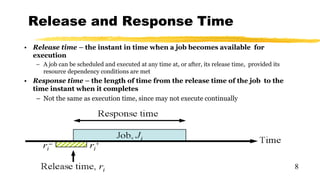
Release and ResponseTime
• Release time – the instant in time when a job becomes available for
execution
– A job can be scheduled and executed at any time at, or after, its release time, provided its
resource dependency conditions are met
• Response time – the length of time from the release time of the job to the
time instant when it completes
– Not the same as execution time, since may not execute continually
8
9.
Deadlines and TimingConstraints
9
• Completion time – the instant at which a job completes execution
• Relative deadline – the maximum allowable job response time
• Absolute deadline – the instant of time by which a job is required to be
completed (often called simply the deadline)
– absolute deadline = release time + relative deadline
– Feasible interval for a job Ji is the interval ( ri, di ]
• Deadlines are examples of timing constraints
10.
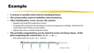
Example
1
0
• A systemto monitor and control a heating furnace
• The system takes 20ms to initialize when turned on
• After initialization, every 100 ms, the system:
– Samples and reads the temperature sensor
– Computes the control-law for the furnace to process temperature readings, determine the
correct flow rates of fuel, air and coolant
– Adjusts flow rates to match computed values
• The periodic computations can be stated in terms of release times of the
jobs computing the control-law: J0, J1, …, Jk, …
– The release time of Jk is 20 + (k × 100) ms
11.
Example
1
1
• Suppose eachjob must complete before the release of the next job:
– Jk’ s relative deadline is 100 ms
– Jk’ s absolute deadline is 20 + ((k + 1) × 100) ms
• Alternatively, each control-law computation may be required to finish
sooner – i.e. the relative deadline is smaller than the time between jobs,
allowing some slack time for other jobs
– Slack time : the difference between the completion time and the earliest possible
completion time
12.
13
Hard vs. SoftReal-Time Systems
• If a job must never miss its deadline, then the
system is described as hard real-time
A timing constraint is hard if the failure to meet it is considered a fatal error; this
definition is based upon the functional criticality of a job
A timing constraint is hard if the usefulness of the results falls off abruptly (or may even
go negative) at the deadline
– If some deadlines can be missed
occasionally, with acceptably low
probability, then the system is
described as soft real-time
– This is a statistical constraint
usefulnes
s
1
deadline
SOFT
HARD
13.
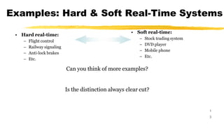
Examples: Hard &Soft Real-Time Systems
1
3
• Hard real-time:
– Flight control
– Railway signaling
– Anti-lock brakes
– Etc.
• Soft real-time:
– Stock trading system
– DVD player
– Mobile phone
– Etc.
Can you think of more examples?
Is the distinction always clear cut?
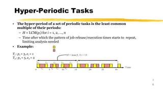
Hyper-Periodic Tasks
1
6
• Thehyper-period of a set of periodic tasks is the least common
multiple of their periods:
– H = LCM(pi) for i = 1, 2, …, n
– Time after which the pattern of job release/execution times starts to repeat,
limiting analysis needed
• Example:
T1 : p1 = 3, e1 = 1
T2 : p2 = 5, e2 = 2
17.
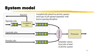
Sporadic and Aperiodic
1
7
•Many real-time systems are required to respond to external events
• The jobs resulting from such events are sporadic or aperiodic
jobs
– A sporadic job has a hard deadlines
– An aperiodic job has either a soft deadline or no deadline
• The release time for sporadic or aperiodic jobs can be modeled as a
random variable with some probability distribution, A(x)
– A(x) gives the probability that the release time of the job is not later than x
• Alternatively, if discussing a stream of similar sporadic/aperiodic jobs,
A(x) can be viewed as the probability distribution of their inter-
release times
[Note: sometimes the terms arrival time (or inter-arrival time) are used instead of release time, due to
their common use in queuing theory]
18.
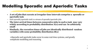
Modelling Sporadic andAperiodic Tasks
1
8
• A set of jobs that execute at irregular time intervals comprise a sporadic or
aperiodic task
– Each sporadic/aperiodic task is a stream of sporadic/aperiodic jobs
• The inter-arrival times between consecutive jobs in such a task may vary
widely according to probability distribution A(x) and can be arbitrarily
small
• Similarly, the execution times of jobs are identically distributed random
variables with some probability distribution B(x)
⇒Sporadic and aperiodic tasks occur in some real-time systems, and greatly
complicate modelling and reasoning
19.
Scheduling
1
9
• Jobs scheduledand allocated resources according to a chosen set of
scheduling algorithms and resource access-control protocols
– Scheduler implements these algorithms
• A scheduler specifically assigns jobs to processors
• A schedule is an assignment of all jobs in the system on the available
processors.
• A valid schedule satisfies the following conditions:
– Every processor is assigned to at most one job at any time
– Every job is assigned at most one processor at any time
– No job is scheduled before its release time
– The total amount of processor time assigned to every job is equal to its maximum or actual
execution time
– All the precedence and resource usage constraints are satisfied
20.
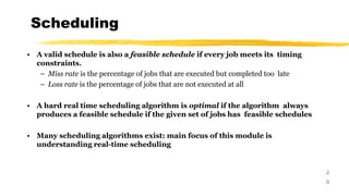
Scheduling
2
0
• A validschedule is also a feasible schedule if every job meets its timing
constraints.
– Miss rate is the percentage of jobs that are executed but completed too late
– Loss rate is the percentage of jobs that are not executed at all
• A hard real time scheduling algorithm is optimal if the algorithm always
produces a feasible schedule if the given set of jobs has feasible schedules
• Many scheduling algorithms exist: main focus of this module is
understanding real-time scheduling
21.
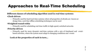
Approaches to Real-TimeScheduling
2
1
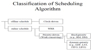
Different classes of scheduling algorithm used in real-time systems:
•Clock-driven
– Primarily used for hard real-time systems where all properties of all jobs are known at
design time, such that offline scheduling techniques can be used
•Weighted round-robin
– Primarily used for scheduling real-time traffic in high-speed, switched networks
•Priority-driven
– Primarily used for more dynamic real-time systems with a mix of timebased and event-
based activities, where the system must adapt to changing conditions and events
Look at the properties of each in turn…
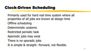
Clock-Driven Scheduling
Primarily usedfor hard real time system where all
properties of all jobs are known at design time
Offline scheduling
Deterministic systems
Restricted periodic task
Aperiodic jobs may exist
There is no sporadic jobs
It is simple & straight –forward, not flexible.
23
24.
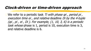
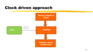
Clock-driven or time-drivenapproach
We refer to a periodic task Ti with phase φi , period pi ,
execution time ei , and relative deadline Di by the 4-tuple
(φi , pi , ei , Di ). For example, (1, 10, 3, 6) is a periodic
task whose phase is 1, period is 10, execution time is 3,
and relative deadline is 6.
24
25.
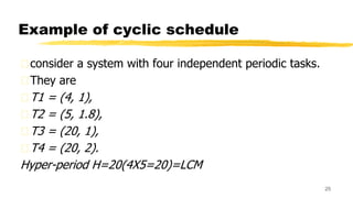
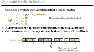
Example of cyclicschedule
consider a system with four independent periodic tasks.
They are
T1 = (4, 1),
T2 = (5, 1.8),
T3 = (20, 1),
T4 = (20, 2).
Hyper-period H=20(4X5=20)=LCM
25
Weighted Round -Robin Mechanism
WRR assumes an average packet length, then computes
a normalized, weighted number of packets to be emitted
by each queue in turn, based on the weight assigned to
each queue.
34.
Weighted Round-Robin Scheduling
3
4
•Regular time-shared applications
– Every job joins a FIFO queue when it is ready for execution
– When the scheduler runs, it schedules the job at the head of the queue to execute for
at most one time slice
• Sometimes called a quantum – typically O(tens of ms)
– If the job has not completed by the end of its quantum, it is preempted and placed at
the end of the queue
– When there are n ready jobs in the queue, each job gets one slice every n time slices
(n time slices is called a round)
– Only limited use in real-time systems
35.
Weighted Round-Robin Scheduling
3
5
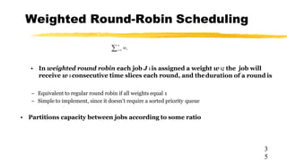
•In weighted round robin each job J i is assigned a weight w i; the job will
receive w i consecutive time slices each round, and theduration of a round is
– Equivalent to regular round robin if all weights equal 1
– Simple to implement, since it doesn’t require a sorted priority queue
• Partitions capacity between jobs according to some ratio
n
i
w
i1
36.
Weighted Round-Robin Scheduling
3
6
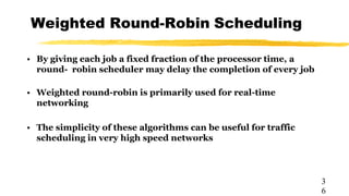
•By giving each job a fixed fraction of the processor time, a
round- robin scheduler may delay the completion of every job
• Weighted round-robin is primarily used for real-time
networking
• The simplicity of these algorithms can be useful for traffic
scheduling in very high speed networks
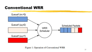
Conventional WRR
z Ina WRR scheduler, tasks are performed in a cyclic
order, in which the time a task can execute within each
round is proportional to the weight assigned to it.
38
39.
Priority-Driven Scheduling
3
9
• Mostscheduling algorithms used in non real-time systems are
priority-driven
– First-In-First-Out
– Last-In-First-Out
– Shortest-Execution-Time-First
– Longest-Execution-Time-First
• Real-time priority scheduling assigns priorities based on deadline or some
other timing constraint:
– Earliest deadline first(EDF)
– Least slack time first(LST)
– Etc.
Assign priority based on release time
Assign priority based on execution time
40.
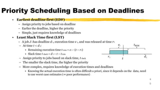
Priority Scheduling Basedon Deadlines
4
0
• Earliest deadline first (EDF)
– Assign priority to jobs based on deadline
– Earlier the deadline, higher the priority
– Simple, just requires knowledge of deadlines
• Least Slack Time first (LST)
– A job J i has deadline d i, execution time e i, and was released at time ri
– At time t < d i:
• Remaining execution time t rem = e i - (t – ri)
• Slack time t slack = d i – t – trem
– Assign priority to jobs based on slack time, t slack
– The smaller the slack time, the higher the priority
– More complex, requires knowledge of execution times and deadlines
• Knowing the actual execution time is often difficult a priori, since it depends on the data, need
to use worst case estimates (⇒ poor performance)
ei
di
ri
t
tREM
41.
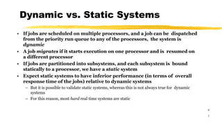
Dynamic vs. StaticSystems
4
1
• If jobs are scheduled on multiple processors, and a job can be dispatched
from the priority run queue to any of the processors, the system is
dynamic
• A job migrates if it starts execution on one processor and is resumed on
a different processor
• If jobs are partitioned into subsystems, and each subsystem is bound
statically to a processor, we have a static system
• Expect static systems to have inferior performance (in terms of overall
response time of the jobs) relative to dynamic systems
– But it is possible to validate static systems, whereas this is not always true for dynamic
systems
– For this reason, most hard real time systems are static
42.
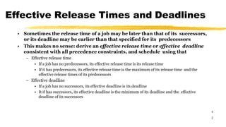
Effective Release Timesand Deadlines
4
2
• Sometimes the release time of a job may be later than that of its successors,
or its deadline may be earlier than that specified for its predecessors
• This makes no sense: derive an effective release time or effective deadline
consistent with all precedence constraints, and schedule using that
– Effective release time
• If a job has no predecessors, its effective release time is its release time
• If it has predecessors, its effective release time is the maximum of its release time and the
effective release times of its predecessors
– Effective deadline
• If a job has no successors, its effective deadline is its deadline
• It if has successors, its effective deadline is the minimum of its deadline and the effective
deadline of its successors
43.
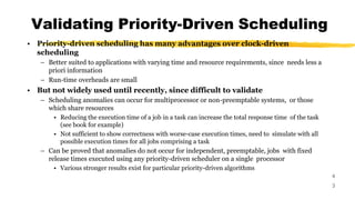
Validating Priority-Driven Scheduling
4
3
•Priority-driven scheduling has many advantages over clock-driven
scheduling
– Better suited to applications with varying time and resource requirements, since needs less a
priori information
– Run-time overheads are small
• But not widely used until recently, since difficult to validate
– Scheduling anomalies can occur for multiprocessor or non-preemptable systems, or those
which share resources
• Reducing the execution time of a job in a task can increase the total response time of the task
(see book for example)
• Not sufficient to show correctness with worse-case execution times, need to simulate with all
possible execution times for all jobs comprising a task
– Can be proved that anomalies do not occur for independent, preemptable, jobs with fixed
release times executed using any priority-driven scheduler on a single processor
• Various stronger results exist for particular priority-driven algorithms
Lecture Outline
4
5
• Assumptions
•Fixed-priority algorithms
– Rate monotonic
– Deadline monotonic
• Dynamic-priority algorithms
– Earliest deadline first
– Least slack time
• Relative merits of fixed- and dynamic-priority scheduling
• Schedulable utilization and proof of schedulability
46.
Assumptions
4
6
• Priority-driven schedulingof periodic tasks on a single processor
• Assume a restricted periodic task model:
– A fixed number of independent periodic tasks exist
• Jobs comprising those tasks:
– Are ready for execution as soon as they are released
– Can be pre-empted at any time
• Never suspend themselves
• New tasks only admitted after an acceptance test; may be rejected
• The period of a task defined as minimum inter-release time of jobs in task
– There are no aperiodic or sporadic tasks
– Scheduling decisions made immediately upon job release and completion
• Algorithms are event driven, not clock driven
• Never intentionally leave a resource idle
– Context switch overhead negligibly small; unlimited priority levels
47.
Dynamic versus StaticSystems
4
7
• In static systems,
– Jobs are partitioned into subsystems, each subsystem bound statically to a processor
– The scheduler for each processor schedules the jobs in its subsystem independent of
the schedulers for the other processors
– Priority-driven uniprocessor systems are applicable to each subsystem of a static
multiprocessor system
• In dynamic systems,
– Jobs are scheduled on multiple processors, and a job can be dispatched to any of the
processors
– Difficult to determine the best- and worst-case performance of dynamic systems, so
most hard real-time systems built are static
• In most cases, the performance of dynamic systems is superior to static
system
• In the worst case, the performance of priority-driven algorithm can be very
poor
48.
Fixed- and Dynamic-PriorityAlgorithms
4
8
• A priority-driven scheduler is an on-line scheduler
– It does not pre-compute a schedule of tasks/jobs: instead assigns priorities to jobs when
released, places them on a run queue in priority order
– When pre-emption is allowed, a scheduling decision is made whenever a job is released or
completed
– At each scheduling decision time, the scheduler updates the run queues and executes the job at
the head of the queue
• Assignment of priority
– Fixed-priority algorithm : to assign the same priority all jobs in each task
– Dynamic-priority algorithm : to assign different priorities to the individual jobs in
each task. Once assigned, the priority of the job does not change (job-level fixed-
priority)
– Job level dynamic-priority : to vary the priority of a job after it has started.
It is usually very inefficient
49.
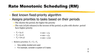
Rate Monotonic Scheduling(RM)
• Best known fixed-priority algorithm
• Assigns priorities to tasks based on their periods
The shorter the period, the higher the priority
The rate (of job releases) is the inverse of the period, so jobs with shorter period
have higher priority
4
9
– T1 = (4,1)
– T2 = (5,2)
– T3 = (20,5)
⇒ rate = 1/4
⇒ rate = 1/5
⇒ rate = 1/20
– Relative priorities: T1 > T2 > T3
• Very widely studied and used
• For example, consider a system of 3 tasks:
50.
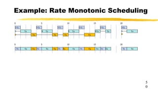
Example: Rate MonotonicScheduling
0 5 10 15 20
T1 T1 T1 T1 T1
T2 T2 T2 T2 T2
T3 T3 T3 T3
T1
T2
0 5 10 15 20
T1 T1
T2 T2 T2 T2 T1 T2
T3 T1 T3 T1 T3 T3 T1 T2
5
0
51.
Deadline Monotonic Scheduling(DM)
5
1
• To assigns task priority according to relative deadlines
– the shorter the relative deadline, the higher the priority
• When relative deadline of every task matches its period, then rate
monotonic and deadline monotonic give identical results
• When the relative deadlines are arbitrary:
– Deadline monotonic can sometimes produce a feasible schedule in cases where rate
monotonic cannot
– But, rate monotonic always fails when deadline monotonic fails
– Deadline monotonic preferred to rate monotonic
• if deadline ≠ period
52.
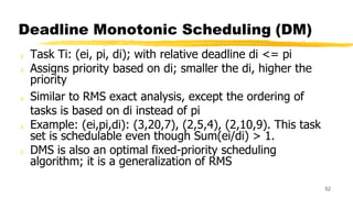
Deadline Monotonic Scheduling(DM)
z Task Ti: (ei, pi, di); with relative deadline di <= pi
z Assigns priority based on di; smaller the di, higher the
priority
z Similar to RMS exact analysis, except the ordering of
tasks is based on di instead of pi
z Example: (ei,pi,di): (3,20,7), (2,5,4), (2,10,9). This task
set is schedulable even though Sum(ei/di) > 1.
z DMS is also an optimal fixed-priority scheduling
algorithm; it is a generalization of RMS
52
Dynamic-Priority Algorithms
5
4
• Earliestdeadline first (EDF)
– To assign priorities to jobs in the tasks according to their absolute deadline
• Least slack time first (LST)
– To check all ready jobs each time a new job is released and
– To order the new job and the existing jobs on their slack time
– Two variations:
• Strict LST – scheduling decisions are made also whenever a queued job’s slack time becomes
smaller than the executing job’s slack time – huge overheads, not used
• Non-strict LST – scheduling decisions made only when jobs release or complete
• First in, first out (FIFO)
– Job queue is first-in-first-out by release time
• Last in, first out (LIFO)
– Job queue is last-in-first-out by release time
• Focus on EDF as commonly used example
Relative Merits
5
6
• Fixed-and dynamic-priority scheduling algorithms have different
properties; neither appropriate for all scenarios
• Algorithms that do not take into account the urgencies of jobs in priority
assignment usually perform poorly
– E.g FIFO, LIFO
• The EDF algorithm gives higher priority to jobs that have missed their
deadlines than to jobs whose deadline is still in the future
– Not necessarily suited to systems where occasional overload unavoidable
• Dynamic algorithms like EDF can produce feasible schedules in cases
where RM and DM cannot. However, it is difficult for the dynamic
algorithms to predict which task will miss their deadlines during overloads.
– But fixed priority algorithms often more predictable, lower overhead
57.
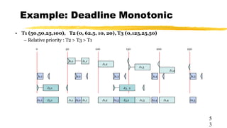
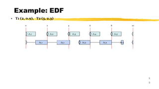
Example: Comparing Different
Algorithms
5
7
•Compare performance of RM, EDF, LST and FIFO scheduling
• Assume a single processor system with 2 tasks:
– T1 = (2, 1)
– T2 = (5, 2.5) H = 10
• The total utilization is 1.0 ⇒ no slack time
– Expect some of these algorithms to lead to missed deadlines!
– This is one of the cases where EDF works better than RM/DM
58.
Example: RM, EDF,LST and FIFO
5
8
• Demonstrate by exhaustive simulation that LST and EDF meet
deadlines, but FIFO and RM don’t
59.
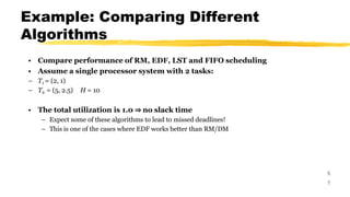
Schedulability Tests
5
9
• Simulatingschedules is both tedious and error-prone… can we
demonstrate correctness without working through the schedule?
• Yes, in some cases. This is a schedulability test
– A test to demonstrate that all deadlines are met, when scheduled using a particular
algorithm
– An efficient schedulability test can be used as an on-line acceptance test; clearly exhaustive
simulation is too expensive
60.
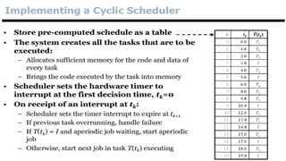
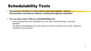
Task scheduling
z Jobsscheduled and allocated resources according to a chosen set
of scheduling algorithms and resource access-control protocols
z – Scheduler implements these algorithms
z • A schedule is an assignment of all jobs in the system on the
available processors.
z • A valid schedule satisfies the following conditions:
z – Every processor is assigned to at most one job at any time
z – Every job is assigned at most one processor at any time
z – No job is scheduled before its release time
z – The total amount of processor time assigned to every job is equal to its
maximum or actual execution time
60
Online- and offlinescheduling:
y Online scheduling is done at run-time based on the
information about the tasks arrived so far.
y Offline scheduling assumes prior knowledge about
arrival times, execution times, and deadlines.
62
63.
Winter 2010- CS244 63
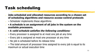
Rate Monotonic (RM) Scheduling
z Well-known technique for scheduling independent
periodic tasks [Liu, 1973].
z Assumptions: low period: high priority
y All tasks that have hard deadlines are periodic.
y All tasks are independent.
y di=pi, for all tasks.
y ci is constant and is known for all tasks.
y The time required for context switching is negligible
64.
Winter 2010- CS244 64
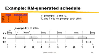
Example: RM-generated schedule
T1 preempts T2 and T3.
T2 and T3 do not preempt each other.
Period Execution Time
T1: 2 0.5
T2: 6 2
T3: 6 1.75
65.
Summary
6
5
Key points:
• Differentpriority scheduling algorithms
– Earliest deadline first, least slack time, rate monotonic, deadline monotonic
– Each has different properties, suited for different scenarios
• Scheduling tests, concept of maximum schedulable utilization
– Examples for different algorithms


![Deadlines and Timing Constraints
9
• Completion time – the instant at which a job completes execution
• Relative deadline – the maximum allowable job response time
• Absolute deadline – the instant of time by which a job is required to be
completed (often called simply the deadline)
– absolute deadline = release time + relative deadline
– Feasible interval for a job Ji is the interval ( ri, di ]
• Deadlines are examples of timing constraints](https://image.slidesharecdn.com/unitiv-real-timecharacteristics1-250919052332-96949b26/85/UNIT-IV-REAL-TIME-CHARACTERISTICS-1-pdf-9-320.jpg)


![Sporadic and Aperiodic
1
7
• Many real-time systems are required to respond to external events
• The jobs resulting from such events are sporadic or aperiodic
jobs
– A sporadic job has a hard deadlines
– An aperiodic job has either a soft deadline or no deadline
• The release time for sporadic or aperiodic jobs can be modeled as a
random variable with some probability distribution, A(x)
– A(x) gives the probability that the release time of the job is not later than x
• Alternatively, if discussing a stream of similar sporadic/aperiodic jobs,
A(x) can be viewed as the probability distribution of their inter-
release times
[Note: sometimes the terms arrival time (or inter-arrival time) are used instead of release time, due to
their common use in queuing theory]](https://image.slidesharecdn.com/unitiv-real-timecharacteristics1-250919052332-96949b26/85/UNIT-IV-REAL-TIME-CHARACTERISTICS-1-pdf-17-320.jpg)


![Winter 2010- CS 244 63
Rate Monotonic (RM) Scheduling
z Well-known technique for scheduling independent
periodic tasks [Liu, 1973].
z Assumptions: low period: high priority
y All tasks that have hard deadlines are periodic.
y All tasks are independent.
y di=pi, for all tasks.
y ci is constant and is known for all tasks.
y The time required for context switching is negligible](https://image.slidesharecdn.com/unitiv-real-timecharacteristics1-250919052332-96949b26/85/UNIT-IV-REAL-TIME-CHARACTERISTICS-1-pdf-63-320.jpg)