6_RealTimeScheduling.pdf

© Lothar Thiele
Computer Engineering and Networks Laboratory
Embedded Systems
6. Aperiodic and Periodic Scheduling

6 - 2
Where we are …
1. Introduction to Embedded Systems
2. Software Development
3. Hardware-Software Interface
4. Programming Paradigms
5. Embedded Operating Systems
6. Real-time Scheduling
7. Shared Resources
8. Hardware Components
9. Power and Energy
10. Architecture Synthesis
Software
Hardware
Hardware-
Software

6 - 4
Basic Terms
Real-time systems
 Hard: A real-time task is said to be hard, if missing its deadline may cause
catastrophic consequences on the environment under control. Examples are
sensory data acquisition, detection of critical conditions, actuator servoing.
 Soft: A real-time task is called soft, if meeting its deadline is desirable for
performance reasons, but missing its deadline does not cause serious damage to
the environment and does not jeopardize correct system behavior. Examples are
command interpreter of the user interface, displaying messages on the screen.

6 - 5
Schedule
Given a set of tasks :
 A schedule is an assignment of tasks to the processor, such that each task is
executed until completion.
 A schedule can be defined as an integer step function
where denotes the task which is executed at time t. If
then the processor is called idle.
 If changes its value at some time, then the processor performs a context
switch.
 Each interval, in which is constant is called a time slice.
 A preemptive schedule is a schedule in which the running task can be arbitrarily
suspended at any time, to assign the CPU to another task according to a
predefined scheduling policy.
,...}
,
{ 2
1 J
J
J 
N
R 
:

)
(t

)
(t

0
)
( 
t

)
(t


6 - 6
Schedule and Timing
 A schedule is said to be feasible, if all task can be completed according to a set
of specified constraints.
 A set of tasks is said to be schedulable, if there exists at least one algorithm that
can produce a feasible schedule.
 Arrival time or release time is the time at which a task becomes ready for
execution.
 Computation time is the time necessary to the processor for executing the
task without interruption.
 Deadline is the time at which a task should be completed.
 Start time is the time at which a task starts its execution.
 Finishing time is the time at which a task finishes its execution.
i
a i
r
i
C
i
d
i
s
i
f

6 - 7
Schedule and Timing
 Using the above definitions, we have
 Lateness represents the delay of a task completion with respect to
its deadline; note that if a task completes before the deadline, its lateness is
negative.
 Tardiness or exceeding time is the time a task stays active after
its deadline.
 Laxity or slack time is the maximum time a task can be delayed
on its activation to complete within its deadline.
i
i
i C
r
d 

i
i
i d
f
L 

)
,
0
max( i
i L
E 
i
i
i
i C
a
d
X 



6 - 8
Schedule and Timing
 Periodic task : infinite sequence of identical activities, called instances or jobs,
that are regularly activated at a constant rate with period . The activation
time of the first instance is called phase .
i

i
T
i

relative deadline
initial phase
arrival time of instance k
period deadline of period k
instance 1 instance 2

6 - 9
Example for Real-Time Model
Computation times: C1 = 9, C2 = 12
Start times: s1 = 0, s2 = 6
Finishing times: f1 = 18, f2 = 28
Lateness: L1 = -4, L2 = 1
Tardiness: E1 = 0, E2 = 1
Laxity: X1 = 13, X2 = 11
task J1 task J2
5 10 15 20 25
r1 r2 d2
d1

6 - 10
Precedence Constraints
 Precedence relations between tasks can be described through an acyclic directed
graph G where tasks are represented by nodes and precedence relations by
arrows. G induces a partial order on the task set.
 There are different interpretations possible:
 All successors of a task are activated (concurrent task execution). We will use this
interpretation in the lecture.
 One successor of a task is activated:
non-deterministic choice.
J1
J2 J3
J5
J4

6 - 11
Precedence Constraints
Example for concurrent activation:
 Image acquisition
 Low level image processing
 Feature/contour extraction
 Pixel disparities
 Object size
 Object recognition
1
acq 2
acq
2
1 edge
edge
shape
disp
H
rec

6 - 12
Classification of Scheduling Algorithms
 With preemptive algorithms, the running task can be interrupted at any time to
assign the processor to another active task, according to a predefined
scheduling policy.
 With a non-preemptive algorithm, a task, once started, is executed by the
processor until completion.
 Static algorithms are those in which scheduling decisions are based on fixed
parameters, assigned to tasks before their activation.
 Dynamic algorithms are those in which scheduling decisions are based on
dynamic parameters that may change during system execution.

6 - 13
Classification of Scheduling Algorithms
 An algorithm is said optimal if it minimizes some given cost function defined
over the task set.
 An algorithm is said to be heuristic if it tends toward but does not guarantee to
find the optimal schedule.
 Acceptance Test: The runtime system decides whenever a task is added to the
system, whether it can schedule the whole task set without deadline violations.
Example for the „domino
effect“, if an acceptance test
wrongly accepted a new task.

6 - 14
Metrics to Compare Schedules
 Average response time:
 Total completion time:
 Weighted sum of response time:
 Maximum lateness:
 Number of late tasks:
 




n
i
i
i
r r
f
n
t
1
1
   
i
i
i
i
c r
f
t min
max 


 


 n
i
i
n
i
i
i
i
w
r
f
w
w
t
1
1
)
(
 
i
i
i
d
f
L 
 max
max
 
 


 

 

otherwise
1
if
0
1
late
i
i
i
n
i
i
d
f
f
miss
f
miss
N

6 - 15
Metrics Example
Average response time:
Total completion time:
Weighted sum of response times:
Number of late tasks:
Maximum lateness:
task J1 task J2
5 10 15 20 25
r1 r2 d2
d1
21
)
24
18
(
2
1 


r
t
28
0
28 


c
t
20
:
1
,
2 3
24
18
2
2
1 


 

w
t
w
w
1
late 
N
1
max 
L

6 - 16
Metrics and Scheduling Example
In schedule (a), the maximum lateness is minimized, but all tasks miss their deadlines.
In schedule (b), the maximal lateness is larger, but only one task misses its deadline.

6 - 17
Real-Time Scheduling of Aperiodic Tasks

6 - 18
Overview Aperiodic Task Scheduling
Scheduling of aperiodic tasks with real-time constraints:
 Table with some known algorithms:
Equal arrival times
non preemptive
Arbitrary arrival times
preemptive
Independent
tasks
EDD
(Jackson)
EDF (Horn)
Dependent
tasks
LDF (Lawler) EDF* (Chetto)

6 - 19
Earliest Deadline Due (EDD)
Jackson’s rule: Given a set of n tasks. Processing in order of non-decreasing
deadlines is optimal with respect to minimizing the maximum lateness.

6 - 20
Example 1:

6 - 21
Jackson’s rule: Given a set of n tasks. Processing in order of non-decreasing
deadlines is optimal with respect to minimizing the maximum lateness.
Proof concept:

6 - 22
Example 2:

6 - 23
Earliest Deadline First (EDF)
Horn’s rule: Given a set of n independent tasks with arbitrary arrival times, any
algorithm that at any instant executes a task with the earliest absolute deadline
among the ready tasks is optimal with respect to minimizing the maximum
lateness.

6 - 24
Example:

6 - 25
Horn’s rule: Given a set of n independent tasks with arbitrary arrival times, any
algorithm that at any instant executes the task with the earliest absolute deadline
among the ready tasks is optimal with respect to minimizing the maximum
lateness.
Concept of proof:
For each time interval it is verified, whether the actual running task is
the one with the earliest absolute deadline. If this is not the case, the task with the
earliest absolute deadline is executed in this interval instead. This operation cannot
increase the maximum lateness.
 
1
, 
t
t

6 - 26
which task is
executing ?
which task has
earliest deadline ?
time slice
slice for
interchange
situation after
interchange

6 - 27
Acceptance test:
 worst case finishing time of task i:
 EDF guarantee condition:
 algorithm:
Algorithm: EDF_guarantee (J, Jnew)
{ J‘=J{Jnew}; /* ordered by deadline */
t = current_time();
f0 = t;
for (each JiJ‘) {
fi = fi-1 + ci(t);
if (fi > di) return(INFEASIBLE);
}
return(FEASIBLE);
}
remaining worst-
case execution time
of task k




i
k
k
i t
c
t
f
1
)
(
i
i
k
k d
t
c
t
n
i 


 
1
)
(
,...,
1

6 - 28
Earliest Deadline First (EDF*)
 The problem of scheduling a set of n tasks with precedence constraints
(concurrent activation) can be solved in polynomial time complexity if tasks are
preemptable.
 The EDF* algorithm determines a feasible schedule in the case of tasks with
precedence constraints if there exists one.
 By the modification it is guaranteed that if there exists a valid schedule at all
then
 a task starts execution not earlier than its release time and not earlier than the
finishing times of its predecessors (a task cannot preempt any predecessor)
 all tasks finish their execution within their deadlines

6 - 31
Modification of deadlines:
 Task must finish the execution time within its deadline.
 Task must not finish the execution later than the maximum start time of its
successor.
 Solution:
task b depends on task a:
 
 
j
i
j
j
i
i J
J
C
d
d
d 

 :
*
min
,
min
*
b
a J
J 
i
j

6 - 32
Modification of release times:
 Task must start the execution not earlier than its release time.
 Task must not start the execution earlier than the minimum finishing time of its
predecessor.
 Solution:
task b depends on task a:
 
 
j
i
i
i
j
j J
J
C
r
r
r 

 :
*
max
,
max
*
b
a J
J 
i
j

6 - 33
Algorithm for modification of release times:
1. For any initial node of the precedence graph set
2. Select a task j such that its release time has not been modified but the release times of
all immediate predecessors i have been modified. If no such task exists, exit.
3. Set
4. Return to step 2
Algorithm for modification of deadlines:
1. For any terminal node of the precedence graph set
2. Select a task i such that its deadline has not been modified but the deadlines of all
immediate successors j have been modified. If no such task exists, exit.
3. Set
4. Return to step 2
 
 
j
i
i
i
j
j J
J
C
r
r
r 

 :
*
max
,
max
*
i
i r
r 
*
i
i d
d 
*
 
 
j
i
j
j
i
i J
J
C
d
d
d 

 :
*
min
,
min
*

6 - 34
Proof concept:
 Show that if there exists a feasible schedule for the modified task set under EDF
then the original task set is also schedulable. To this end, show that the original
task set meets the timing constraints also. This can be done by using ,
; we only made the constraints stricter.
 Show that if there exists a schedule for the original task set, then also for the
modified one. We can show the following: If there exists no schedule for the
modified task set, then there is none for the original task set. This can be done by
showing that no feasible schedule was excluded by changing the deadlines and
release times.
 In addition, show that the precedence relations in the original task set are not
violated. In particular, show that
 a task cannot start before its predecessor and
 a task cannot preempt its predecessor.
i
i r
r 
*
i
i d
d 
*

6 - 35
Real-Time Scheduling of Periodic Tasks

6 - 36
Overview
Table of some known preemptive scheduling algorithms for periodic tasks:
Deadline equals
period
Deadline smaller than
period
static
priority
RM
(rate-monotonic)
DM
(deadline-monotonic)
dynamic
priority
EDF EDF*

6 - 37
Model of Periodic Tasks
 Examples: sensory data acquisition, low-level actuation, control loops, action
planning and system monitoring.
 When an application consists of several concurrent periodic tasks with individual
timing constraints, the OS has to guarantee that each periodic instance is
regularly activated at its proper rate and is completed within its deadline.
 Definitions:
: denotes a set of periodic tasks
: denotes a periodic task
: denotes the jth instance of task i
: denote the release time, start time, finishing time, absolute
deadline of the jth instance of task i
: denotes the phase of task i (release time of its first instance)
: denotes the relative deadline of task i
: denotes the period of task i

i

j
i,

j
i
j
i
j
i
j
i d
f
s
r ,
,
,
, ,
,
,
i

i
D
i
T

6 - 38
 The following hypotheses are assumed on the tasks:
 The instances of a periodic task are regularly activated at a constant rate. The
interval between two consecutive activations is called period. The release times
satisfy
 All instances have the same worst case execution time
 All instances of a periodic task have the same relative deadline . Therefore, the
absolute deadlines satisfy
 Often, the relative deadline equals the period (implicit deadline), and
therefore
  i
i
i
j
i D
T
j
d 



 1
,
  i
i
j
i T
j
r 1
, 



i
C
i
T
i
D
i
i T
D 
i
i
j
i jT
d 


,

6 - 39
 The following hypotheses are assumed on the tasks (continued):
 All periodic tasks are independent; that is, there are no precedence relations and
no resource constraints.
 No task can suspend itself, for example on I/O operations.
 All tasks are released as soon as they arrive.
 All overheads in the OS kernel are assumed to be zero.
 Example:
i

i

i
T
1
,
i
r 2
,
i
r
i
D
3
,
i
s 3
,
i
f
3
,
i

i
C

6 - 40
Rate Monotonic Scheduling (RM)
 Assumptions:
 Task priorities are assigned to tasks before execution and do not change over time
(static priority assignment).
 RM is intrinsically preemptive: the currently executing job is preempted by a job of
a task with higher priority.
 Deadlines equal the periods .
Rate-Monotonic Scheduling Algorithm: Each task is assigned a priority. Tasks with
higher request rates (that is with shorter periods) will have higher priorities. Jobs of
tasks with higher priority interrupt jobs of tasks with lower priority.
i
i T
D 

6 - 41
Periodic Tasks
Example: 2 tasks, deadlines = periods, utilization = 97%

6 - 42
Optimality: RM is optimal among all fixed-priority assignments in the sense that
no other fixed-priority algorithm can schedule a task set that cannot be
scheduled by RM.
 The proof is done by considering several cases that may occur, but the main
ideas are as follows:
 A critical instant for any task occurs whenever the task is released
simultaneously with all higher priority tasks. The tasks schedulability can easily
be checked at their critical instants. If all tasks are feasible at their critical
instant, then the task set is schedulable in any other condition.
 Show that, given two periodic tasks, if the schedule is feasible by an arbitrary
priority assignment, then it is also feasible by RM.
 Extend the result to a set of n periodic tasks.

6 - 43
Proof of Critical Instance
Lemma: For any task, the critical instant occurs if a job is simultaneously
released with all higher priority jobs.
Definition: A critical instant of a task is the time at which the release of a job
will produce the largest response time.
Proof sketch: Start with 2 tasks 1 and 2 .
Response time of a job of 2 is delayed by jobs of 1 of higher priority:
C2+2C1
•2
•1
t

6 - 44
Proof of Critical Instance
Delay may increase if 1 starts earlier:
C2+3C1
•2
•1
t
Maximum delay achieved if 2 and 1 start simultaneously.
Repeating the argument for all higher priority tasks of some task 2 :
• The worst case response time of a job occurs when it
• is released simultaneously with all higher-priority jobs.

6 - 45
Proof of RM Optimality (2 Tasks)
We have two tasks 1, 2 with periods T1 < T2.
•1
•2
t
• Schedule is feasible if C1+C2  T1 and (A)
C1
C2
T1
Consider two cases A and B:
Case A: Assume RM is not used  prio(2) is highest:
Define F= T2/T1: the number of periods of 1 fully contained in T2
C2  T2
T2

6 - 46
•1
•2 t
T2
FT1
Case B: Assume RM is used  prio(1) is highest:
C1
Schedulable is feasible if
FC1+C2+min(T2–FT1, C1)  T2 and C1  T1 (B)
Given tasks 1 and 2 with T1 < T2, then if the schedule is feasible by an
arbitrary fixed priority assignment, it is also feasible by RM.
We need to show that (A)  (B):
T2–FT1
C1+C2  T1  C1  T1
C1+C2  T1  FC1+C2  FC1+FC2  FT1 
FC1+C2+min(T2–FT1, C1)  FT1 +min(T2–FT1, C1)  min(T2, C1+FT1)  T2

6 - 47
•1
•2 t
T2
FT1
C1
T2–FT1
C1+C2  T1  C1  T1
C1+C2  T1  FC1+C2  FC1+FC2  FT1 

6 - 48
•1
•2 t
T2
FT1
C1
T2–FT1
C1+C2  T1  C1  T1
C1+C2  T1  FC1+C2  FC1+FC2  FT1 

6 - 49
•1
•2 t
T2
FT1
C1
T2–FT1
C1+C2  T1  C1  T1
C1+C2  T1  FC1+C2  FC1+FC2  FT1 

6 - 50
•1
•2 t
T2
FT1
C1
T2–FT1
C1+C2  T1  C1  T1
C1+C2  T1  FC1+C2  FC1+FC2  FT1 

6 - 52
Schedulability analysis: A set of periodic tasks is schedulable with RM if
This condition is sufficient but not necessary.
The term denotes the processor
utilization factor U which is the fraction of processor
time spent in the execution of the task set.
 
1
2 /
1
1




n
n
i i
i n
T
C



n
i i
i
T
C
U
1

6 - 53
Proof of Utilization Bound (2 Tasks)
Proof Concept: Compute upper bound on utilization U such that the task set is
still schedulable:
 assign priorities according to RM;
 compute upper bound Uup by increasing the computation time C2 to just
meet the deadline of 2; we will determine this limit of C2 using the results
of the RM optimality proof.
 minimize upper bound with respect to other task parameters in order to
find the utilization below which the system is definitely schedulable.
We have two tasks 1, 2 with periods T1 < T2.
Define F= T2/T1: number of periods of 1 fully contained in T2

6 - 54
As before:
Utilization:
•1
•2 t
T2
FT1
C1
Schedulable if FC1+C2+min(T2–FT1, C1)  T2 and C1  T1
T2–FT1

6 - 55

6 - 56
Minimize utilization bound w.r.t C1:
 If C1  T2–FT1 then U decreases with increasing C1
 If T2–FT1  C1 then U decreases with decreasing C1
 Therefore, minimum U is obtained with C1 = T2–FT1 :
We now need to minimize w.r.t. G =T2/T1 where F = T2/T1 and T1 < T2. As F is
integer, we first suppose that it is independent of G = T2/T1. Then we obtain

6 - 57
Minimizing U with respect to G yields
If we set F = 1, then we obtain
It can easily be checked, that all other integer values for F lead to a larger upper
bound on the utilization.

6 - 58
Deadline Monotonic Scheduling (DM)
 Assumptions are as in rate monotonic scheduling, but deadlines may be smaller
than the period, i.e.
Algorithm: Each task is assigned a priority. Tasks with smaller relative deadlines will
have higher priorities. Jobs with higher priority interrupt jobs with lower priority.
 Schedulability Analysis: A set of periodic tasks is schedulable with DM if
This condition is sufficient but not necessary (in general).
 
1
2 /
1
1




n
n
i i
i n
D
C
i
i
i T
D
C 


6 - 59
Deadline Monotonic Scheduling (DM) - Example
1 10
1
1 10
2
1 10
3
1 10
4
U = 0.874   757
.
0
1
2
08
.
1 /
1
1






n
n
i i
i n
D
C

6 - 60
There is also a necessary and sufficient schedulability test which is computationally
more involved. It is based on the following observations:
 The worst-case processor demand occurs when all tasks are released
simultaneously; that is, at their critical instances.
 For each task i, the sum of its processing time and the interference imposed
by higher priority tasks must be less than or equal to .
 A measure of the worst case interference for task i can be computed as the
sum of the processing times of all higher priority tasks released before some
time where tasks are ordered according to :
i
D
t
j
i
j j
i C
T
t
I 

 








1
1
n
m D
D
n
m 



6 - 61
 The longest response time of a job of a periodic task i is computed, at the
critical instant, as the sum of its computation time and the interference due to
preemption by higher priority tasks:
 Hence, the schedulability test needs to compute the smallest that satisfies
for all tasks i. Then, must hold for all tasks i.
 It can be shown that this condition is necessary and sufficient.
i
i D
R 
j
i
j j
i
i
i C
T
R
C
R 

 









1
1
i
R
i
i
i I
C
R 

i
R

6 - 62
The longest response times of the periodic tasks i can be computed iteratively
by the following algorithm:
i
R
Algorithm: DM_guarantee ()
{ for (each i){
I = 0;
do {
R = I + Ci;
if (R > Di) return(UNSCHEDULABLE);
I = j=1,…,(i-1)R/Tj Cj;
} while (I + Ci > R);
}
return(SCHEDULABLE);
}

6 - 63
DM Example
Example:
 Task 1:
 Task 2:
 Task 3:
 Task 4:
 Algorithm for the schedulability test for task 4:
 Step 0:
 Step 1:
 Step 2:
 Step 3:
 Step 4:
 Step 5:
3
;
4
;
1 1
1
1 

 D
T
C
4
;
5
;
1 2
2
2 

 D
T
C
5
;
6
;
2 3
3
3 

 D
T
C
10
;
11
;
1 4
4
4 

 D
T
C
1
4 
R
5
4 
R
6
4 
R
7
4 
R
9
4 
R
10
4 
R

6 - 64
DM Example
1 10
1
1 10
2
1 10
3
1 10
4
U = 0.874   757
.
0
1
2
08
.
1 /
1
1






n
n
i i
i n
D
C

6 - 65
EDF Scheduling (earliest deadline first)
 Assumptions:
 dynamic priority assignment
 intrinsically preemptive
 Algorithm: The currently executing task is preempted whenever another
periodic instance with earlier deadline becomes active.
 Optimality: No other algorithm can schedule a set of periodic tasks if the set that
can not be scheduled by EDF.
 The proof is simple and follows that of the aperiodic case.
  i
i
i
j
i D
T
j
d 



 1
,

6 - 66
Periodic Tasks

6 - 67
EDF Scheduling
A necessary and sufficient schedulability test for :
A set of periodic tasks is schedulable with EDF if and only if
The term denotes the average processor utilization.
1
1




U
T
C
n
i i
i



n
i i
i
T
C
U
1
i
i T
D 

6 - 68
EDF Scheduling
 If the utilization satisfies , then there is no valid schedule: The total
demand of computation time in interval is
and therefore, it exceeds the available processor time in this interval.
 If the utilization satisfies , then there is a valid schedule.
We will proof this fact by contradiction: Assume that deadline is missed at some
time t2 . Then we will show that the utilization was larger than 1.
1

U
n
T
T
T
T 


 ...
2
1
T
UT
T
T
C
n
i i
i



1
1

U

6 - 70
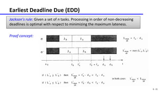
EDF Scheduling
 If the deadline was missed at t2 then define t1 as a time before t2 such that (a) the processor is
continuously busy in [t1, t2 ] and (b) the processor only executes tasks that have their arrival
time AND their deadline in [t1, t2 ].
 Why does such a time t1 exist? We find such a t1 by starting at t2 and going backwards in time,
always ensuring that the processor only executed tasks that have their deadline before or at t2 :
 Because of EDF, the processor will be busy shortly before t2 and it executes on the task that has
deadline at t2.
 Suppose that we reach a time such that shortly before the processor works on a task with deadline
after t2 or the processor is idle, then we found t1: We know that there is no execution on a task with
deadline after t2 .
 But it could be in principle, that a task that arrived before t1 is executing in [t1, t2 ].
 If the processor is idle before t1, then this is clearly not possible due to EDF (the processor is not idle, if
there is a ready task).
 If the processor is not idle before t1, this is not possible as well. Due to EDF, the processor will always
work on the task with the closest deadline and therefore, once starting with a task with deadline after t2
all task with deadlines before t2 are finished.

6 - 72
EDF Scheduling
 Within the interval the total computation time demanded by the periodic
tasks is bounded by
 Since the deadline at time is missed, we must have:
 
2
1,t
t
 U
t
t
C
T
t
t
C
T
t
t
t
t
C
n
i
i
i
n
i
i
i
p 1
2
1
1
2
1
1
2
2
1 )
,
( 








 
 
 

    1
, 1
2
2
1
1
2 




 U
U
t
t
t
t
C
t
t p
number of complete periods
of task i in the interval
2
t

6 - 73
Periodic Task Scheduling

6 - 74
Real-Time Scheduling of Mixed Task Sets

6 - 75
Problem of Mixed Task Sets
In many applications, there are aperiodic as well as periodic tasks.
 Periodic tasks: time-driven, execute critical control activities with hard timing
constraints aimed at guaranteeing regular activation rates.
 Aperiodic tasks: event-driven, may have hard, soft, non-real-time requirements
depending on the specific application.
 Sporadic tasks: Offline guarantee of event-driven aperiodic tasks with critical
timing constraints can be done only by making proper assumptions on the
environment; that is by assuming a maximum arrival rate for each critical event.
Aperiodic tasks characterized by a minimum interarrival time are called
sporadic.

6 - 76
Background Scheduling
Background scheduling is a simple solution for RM and EDF:
 Processing of aperiodic tasks in the background, i.e. execute if there are no
pending periodic requests.
 Periodic tasks are not affected.
 Response of aperiodic tasks may be prohibitively long and there is no possibility to
assign a higher priority to them.
 Example:

6 - 77
Background Scheduling
Example (rate monotonic periodic schedule):

6 - 78
Rate-Monotonic Polling Server
 Idea: Introduce an artificial periodic task whose purpose is to service aperiodic
requests as soon as possible (therefore, “server”).
 Function of polling server (PS)
 At regular intervals equal to , a PS task is instantiated. When it has the highest
current priority, it serves any pending aperiodic requests within the limit of its
capacity .
 If no aperiodic requests are pending, PS suspends itself until the beginning of the
next period and the time originally allocated for aperiodic service is not preserved
for aperiodic execution.
 Its priority (period!) can be chosen to match the response time requirement for
the aperiodic tasks.
 Disadvantage: If an aperiodic requests arrives just after the server has
suspended, it must wait until the beginning of the next polling period.
s
T
s
C

6 - 79
Example:
server has current
highest priority
and checks the
queue of tasks
remaining budget is lost

6 - 80
Schedulability analysis of periodic tasks:
 The interference by a server task is the same as the one introduced by an
equivalent periodic task in rate-monotonic fixed-priority scheduling.
 A set of periodic tasks and a server task can be executed within their deadlines if
 Again, this test is sufficient but not necessary.
 
1
2
)
1
( )
1
/(
1
1



 

 n
n
i i
i
s
s n
T
C
T
C

6 - 81
Guarantee the response time of aperiodic requests:
 Assumption: An aperiodic task is finished before a new aperiodic request
arrives.
 Computation time , deadline
 Sufficient schedulability test:
a
s
s
a D
T
C
C







 )
1
(
a
C a
D
The aperiodic task arrives
shortly after the activation
of the server task. Maximal number of
necessary server periods.
If the server task
has the highest
priority there is a
necessary test also.

6 - 82
EDF – Total Bandwidth Server
Total Bandwidth Server:
 When the kth aperiodic request arrives at time t = rk, it receives a deadline
where Ck is the execution time of the request and Us is the server utilization
factor (that is, its bandwidth). By definition, d0=0.
 Once a deadline is assigned, the request is inserted into the ready queue of
the system as any other periodic instance.
s
k
k
k
k
U
C
d
r
d 
  )
,
max( 1

6 - 84
Example:
1
,
25
.
0
,
75
.
0 


 s
p
s
p U
U
U
U

6 - 85
Schedulability test:
Given a set of n periodic tasks with processor utilization Up and a total bandwidth
server with utilization Us, the whole set is schedulable by EDF if and only if
Proof:
 In each interval of time , if Cape is the total execution time demanded by
aperiodic requests arrived at t1 or later and served with deadlines less or equal to
t2, then
1

 s
p U
U
]
,
[ 2
1 t
t
s
ape U
t
t
C )
( 1
2 


6 - 86
If this has been proven, the proof of the schedulability test follows closely that of the
periodic case.
Proof of lemma:
 
)
(
)
,
max(
))
,
max(
(
1
2
1
1
1
1
2
2
1
2
1
t
t
U
d
r
d
U
d
r
d
U
C
C
s
k
k
k
s
k
k
k
k
k
k
s
k
k
k
k
ape














6_RealTimeScheduling.pdf

Recommended

Recommended

More Related Content

Similar to 6_RealTimeScheduling.pdf

Similar to 6_RealTimeScheduling.pdf (20)

More from Tigabu Yaya

More from Tigabu Yaya (20)

Recently uploaded

Recently uploaded (20)

6_RealTimeScheduling.pdf