Unit II and III

1. Computer Vision (21AM504) - Unit II & III
Topics not covered in PPT
1
Unit II
1 Affinity measures: Some model of segmentation simply requires a weight to place on each edge of the
graph; these weights are usually called affinity measures.
Clearly, the affinity measure depends on the problem at hand. The weight of an arc connecting similar
nodes should be large, and the weight on an arc connecting very different nodes should be small. It is
fairly easy to come up with affinity measures with these properties for a variety of important cases, and
we can construct an affinity function for a combination of cues by forming a product of powers of these
affinity functions.
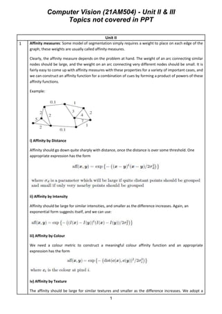
Example:
i) Affinity by Distance
Affinity should go down quite sharply with distance, once the distance is over some threshold. One
appropriate expression has the form
ii) Affinity by Intensity
Affinity should be large for similar intensities, and smaller as the difference increases. Again, an
exponential form suggests itself, and we can use:
iii) Affinity by Colour
We need a colour metric to construct a meaningful colour affinity function and an appropriate
expression has the form
iv) Affinity by Texture
The affinity should be large for similar textures and smaller as the difference increases. We adopt a

2. Computer Vision (21AM504) - Unit II & III
Topics not covered in PPT
2
collection of filters f1, . . ., fn, and describe textures by the outputs of these filters, which should span a
range of scales and orientations. Now for most textures, the filter outputs will not be the same at each
point in the texture
we use an exponential form:
v) Affinity by Motion
In the case of motion, the nodes of the graph are going to represent a pixel in a particular image in the
sequence. It is difficult to estimate the motion at a particular pixel accurately; instead, it makes sense to
construct a distribution over the possible motions. The quality of motion estimate available depends on
what the neighbourhood of the pixel looks like.
If we define a similarity measure for an image motion v at a pixel x to be
We have a measure that will be near one for a good value of the motion and near zero for a poor one.
This can be massaged into a probability distribution by ensuring that it somes to one, so we have
Now we need to obtain an affinity measure from this. The arcs on the graph will connect pixels that are
“nearby” in space and in time. For each pair of pixels, the affinity should be high if the motion pattern
around the pixels could look similar, and low otherwise. This suggests using a correlation measure for
the affinity.
2 Normalized Cuts
An approach to cut the graph into two connected components such that the cost of the cut is a
small fraction of the total affinity within each group.
We can formalise this as decomposing a weighted graph V into two components A and B, and
scoring the decomposition with
(where cut(A,B) is the sum of weights of all edges in V that have one end in A and the other in
B, and assoc(A, V ) is the sum of weights of all edges that have one end in A). This score will be
small if the cut separates two components that have very few edges of low weight between
them and many internal edges of high weight.
We would like to find the cut with the minimum value of this criterion, called a normalized cut.
 This problem is too difficult to solve in this form, because we would need to look at

3. Computer Vision (21AM504) - Unit II & III
Topics not covered in PPT
3
every graph cut — it’s a combinatorial optimization problem, so we can’t use continuity
arguments to reason about how good a neighbouring cut is given the value of a
particular cut.
3 Human Vision: Stereopsis
Unlike the cameras rigidly attached to a passive stereo rig, the two eyes of a person can rotate
in their sockets. At each instant, they fixate on a particular point in space, i.e., they rotate so
that its two images form in the centers of the eyes’ foveas.
Below Figure illustrates a simplified, two-dimensional situation.
If l and r denote the angles between the vertical planes of symmetry of two eyes and two rays
passing through the same scene point, we define the corresponding disparity as d = r − l.
It is an elementary exercise in trigonometry to show that d = D −F, where D denotes the angle
between these rays, and F is the angle between the two rays passing through the fixated point.
Points with zero disparity lie on the ViethM¨uller circle that passes through the fixated point
and the anterior nodal points of the eyes.
Points lying inside this circle have a positive (or convergent) disparity, points lying outside it
have, a negative (or divergent) disparity, and the locus of all points having a given disparity d
forms, as d varies, the pencil of all circles passing through the two eyes’ nodal points. This
property is clearly sufficient to rank-order in depth dots that are near the fixation point.
However, it is also clear that the vergence angles between the vertical median plane of
symmetry of the head and the two fixation rays must be known in order to reconstruct the
absolute position of scene points.
4 Epipolar Geometry

4. Computer Vision (21AM504) - Unit II & III
Topics not covered in PPT
4
5 Trinocular Stereo
Adding a third camera eliminates (in large part) the ambiguity inherent in two view point
matching. In essence, the third image can be used to check hypothetical matches between the
first two pictures (as shown in below figure, the three-dimensional point associated with such
a match is first reconstructed then reprojected into the third image.
If no compatible point lies nearby, then the match must be wrong. In fact, the
reconstruction/reprojection process can be avoided by noting, that, given three weakly (and a

5. Computer Vision (21AM504) - Unit II & III
Topics not covered in PPT
5
fortiori strongly) calibrated cameras and two images of a point, one can always predict its
position in a third image by intersecting the corresponding epipolar lines.
The trifocal tensor can be used to also predict the tangent line to some image curve in one
image given the corresponding tangents in the other images: given matching tangents l2 and l3
in images 2 and 3, we can reconstruct the tangent l1 in image number 1 is
Unit III
1. What is tracking? List and explain the various applications of tracking. Describe tracking
people.
Tracking:
Tracking is the problem of generating an inference about the motion of an object given a
sequence of images.
Good solutions to this problem have a variety of applications:
• Motion Capture: if we can track a moving person accurately, then we can make an accurate
record of their motions. Once we have this record, we can use it to drive a rendering process;

6. Computer Vision (21AM504) - Unit II & III
Topics not covered in PPT
6
for example, we might control a cartoon character, thousands of virtual extras in a crowd
scene, or a virtual stunt avatar. Furthermore, we could modify the motion record to obtain
slightly different motions. This means that a single performer can produce sequences they
wouldn’t want to do in person.
• Recognition From Motion: the motion of objects is quite characteristic. We may be able to
determine the identity of the object from its motion; we should be able to tell what it’s doing.
• Surveillance: knowing what objects are doing can be very useful. For example, different kinds
of trucks should move in different, fixed patterns in an airport; if they do not, then something
is going very wrong. Similarly, there are combinations of places and patterns of motions that
should never occur (no truck should ever stop on an active runway, say). It could be helpful to
have a computer system that can monitor activities and give a warning if it detects a problem
case.
• Targeting: a significant fraction of the tracking literature is oriented towards (a) deciding
what to shoot and (b) hitting it. Typically, this literature describes tracking using radar or infra-
red signals (rather than vision), but the basic issues are the same — what do we infer about an
object’s future position from a sequence of measurements? (i.e. where should we aim?)
In typical tracking problems, we have a model for the object’s motion, and some set of
measurements from a sequence of images. These measurements could be the position of
some image points, the position and moments of some image regions, or pretty much anything
else. They are not guaranteed to be relevant, in the sense that some could come from the
object of interest and some might come from other objects, or from noise.
Tracking People
 People are typically modelled as a collection of body segments, connected with rigid
transformations.
 These segments can be modelled as cylinders — in which case, we can ignore the top
and bottom of the cylinder and any variations in view, and represent the cylinder as an
image rectangle of fixed size — or as ellipsoids.
 The state of the tracker is then given by the rigid body transformations connecting
these body segments (and perhaps, various velocities and accelerations associated with
them).
 Both particle filters and (variants of) Kalman filters have been used to track people.
Each approach can be made to succeed, but neither is particularly robust.
2 Explain vehicle tracking application in detail
Vehicle tracking
Systems that can track cars using video from fixed cameras can be used to predict traffic
volume and flow; the ideal is to report on, and act to prevent, traffic problems as quickly as
possible. A number of systems can track vehicles successfully. The crucial issue is initiating a
track automatically.
• Sullivan et al. construct a set of regions of interest (ROI’s) in each frame. Because the
camera is fixed, these regions of interest can be chosen to span each lane, this means that
almost all vehicles must pass directly through a region of interest in a known direction.

7. Computer Vision (21AM504) - Unit II & III
Topics not covered in PPT
7
Their system then watches for characteristic edge signatures in the ROI that indicate
the presence of a vehicle. These signatures can alias slightly — typically, a track is initiated
when the front of the vehicle enters the ROI, another is initiated when the vehicle lies in the
ROI, and a third is initiated close to the vehicle’s leaving — because some of the vehicle’s
edges are easily mistaken for others.
Each initiated track is tracked for a sequence of frames, during which time it
accumulates a quality score — essentially, an estimate of the extent to which predictions of
future position were accurate.
If this quality score is sufficiently high, the track is accepted as an hypothesis. An
exclusion region in space and time is constructed around each hypothesis, such that there can
be only one track in this region, and if the regions overlap, the track with the highest quality is
chosen.
The requirement that the exclusion regions do not overlap derives from the fact that
two cars can’t occupy the same region of space at the same time. Once a track has passed
these tests, the position in which and the time at which it will pass through another ROI can be
predicted. The track is finally confirmed or rejected by comparing this ROI at the appropriate
time with a template that predicts the car’s appearance. Typically, relatively few tracks that are
initiated reach this stage.
• An alternative method for initiating car tracks is to track individual features, and then
group those tracks into possible cars. Beymer et al. use this strategy rather successfully.
Because the road is plane and the camera is fixed, the homography connecting the road plane
and the camera can be determined. This homography can be used to determine the distance
between points; and points can lie together on a car only if this distance doesn’t change with
time.
Their system tracks corner points, identified using a second moment matrix, using a
Kalman filter. Points are grouped using a simple algorithm using a graph abstraction: each
feature track is a vertex, and edges represent a grouping relationship between the tracks.
When a new feature comes into view — and a track is thereby initiated — it is given an
edge joining it to every feature track that appears nearby in that frame. If, at some future time,
the distance between points in a track changes by too much, the edge is discarded.
An exit region is defined near where vehicles will leave the frame. When tracks reach
this exit region, connected components are defined to be vehicles. This grouper is successful,
both in example images and in estimating traffic parameters over long sequences.
The ground plane to camera transformation can provide a great deal of information;
once an object has been tracked, we can use this transformation to reason about spatial layout
and occlusion.
• Remagnino et al. track vehicles and pedestrians — pedestrians in coarse scale images
are represented with a closed B-spline curve, whose control points are tracked with a Kalman
filter; the B-spline tracks edge data, using a fairly narrow gate around a set of discrete points
along the spline and then reconstruct spatial relations using this homography. The advantage
of this approach is that one can engage in explicit occlusion reasoning, so that even
pedestrians partially occluded by a car can be tracked. Another use of the homography makes
it possible to track cars from moving vehicles. In this case, there are two issues to manage:
firstly, the motion of the camera platform (so-called ego-motion); and secondly, the motion of
other vehicles.
• Maybank et al. estimate the ego-motion by matching views of the road to one another
from frame to frame. With an estimate of the homography and of the ego-motion, we can now
refer tracks of other moving vehicles into the road coordinate system to come up with

8. Computer Vision (21AM504) - Unit II & III
Topics not covered in PPT
8
reconstructions of all vehicles visible on the road from a moving vehicle