Adaline and Madaline are adaptive linear neuron models. Adaline is a single linear neuron that can be trained with the least mean square algorithm or stochastic gradient descent. Madaline is a network of multiple Adalines that can be trained with Madaline Rule II to perform non-linear functions like XOR. Madaline has applications in tasks like echo cancellation, signal prediction, adaptive beamforming antennas, and translation-invariant pattern recognition. Conjugate gradient descent converges faster than gradient descent for minimizing quadratic functions.

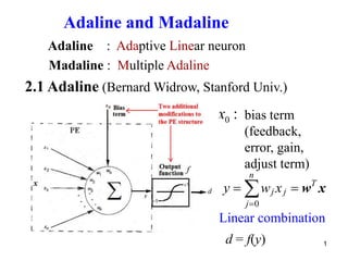
1. 1
Adaline and Madaline
Adaline : Adaptive Linear neuron
Madaline : Multiple Adaline
2.1 Adaline (Bernard Widrow, Stanford Univ.)
bias term
(feedback,
error, gain,
adjust term)
0
w x
n
T
j j
j
y w x

 

0 :
x
Linear combination
d = f(y)

2. 2
2.1.1 Least Mean Square (LMS) Learning
◎ Input vectors :
Ideal outputs :
Actual outputs :
1 2
{ , , , }
L

x x x
1 2
{ , , , }
L
d d d

1 2
{ , , , }
L
y y y

   
2
2
2 2
1
2
1
2 -- (2.4)
L
T
k k k k k k
k
T T T
k k k k k
ε ε d y d
L
d d

    
  
 w x
w x x w x w
Mean square error:
Let 2
, ,
k k k
ξ ε d
 
p x :
x xT
k k
R  correlation
matrix
Assume the output function: f(y) = y = d

3. 3
Let
( )
2 2 0.
d
R
d

  
w
w p
w
* 1
.
R

w p
Obtain
Practical difficulties of analytical formula :
1. Large dimensions - difficult to calculate
2. < > expected value - Knowledge of probabilities
1
R
Idea: *
argmin ( )
 
w
w w
2
(2.4) 2
T T
k
d R

   
w w p w

4. 4
The graph of is a
paraboloid.
2
( ) 2
T T
k
d R
   
w w w p w
2.1.2 Steepest Descent

5. 5
Steps: 1. Initialize weight values
2. Determine the steepest descent direction
Let
3. Modify weight values
4. Repeat 2~3.
( 1) ( ) ( ), : step size
t t t
   
w w w
 
( ( ))
( ( )) 2( ( ))
( )
d t
t R t
d t


    
w
w
w p w
w
0
( )
t
w
No calculation of
( ) ( ( ))
t t
  
w
w w

Drawbacks: i) To know R and p is equivalent to
knowing the error surface in advance. ii) Steepest
descent training is a batch training method.
1
R

6. 6
2.1.3 Stochastic Gradient Descent
Approximate by randomly
selecting one training example at a time
1. Apply an input vector
2.
3.
4.
5. Repeat 1~4 with the next input vector
( ( )) 2( ( ))
t R t
  

w
w p w
k
x
2 2 2
( ) ( ) ( ( ) )
T
k k k k k
ε t d y d t
    
w x
2 2
( ) ( ) ( )
2( ( ) ) 2 ( )
k k
t
k k k k k
t ε t ε t
d t ε t

    
     
w w w
w x x x
( 1) ( ) 2 ( )
k k
t t με t
  
w w x
and R
p
No calculation of

7. 7
○ Practical Considerations:
(a) No. of training vectors, (b) Stopping criteria
(c) Initial weights, (d) Step size
Drawback: time consuming.
Improvement: mini-batch training method.

8. 2.1.4 Conjugate Gradient Descent
-- Drawback: can only minimize quadratic functions,
e.g., 1
( )
2
T T
f A c
  
w w w b w
Advantage: guarantees to find the optimum solution in
at most n iterations, where n is the size of matrix A.
A-Conjugate Vectors:
Let square, symmetric, positive-definite matrix.
Vectors are A-conjugate
if
{ (0), (1), , ( 1)}
S n
  
s s s
( ) ( ) 0,
s s
T
i A j i j
  
:
n n
A 
* If A = I (identity matrix), conjugacy = orthogonality.

9. Set S forms a basis for space .
n
R
The solution in can be written as
1
0
( )
n
i
i
a i



 
w s

w n
R
• The conjugate-direction method for minimizing f(w) is
defined by ( 1) ( ) ( ) ( ), 0,1, , 1
i i i i i n

     
w w s
where w(0) is an arbitrary starting vector.
is determined by
( )
i
 min ( ( ) ( ))
f i i



w s
Let ( ) ( ) ( ) ( 1), 1,2, , 1 (A)
i i i i i n

      
s r s
Define , which is in the steepest
descent direction of
( ) ( )
i A i
 
r b w
( ( ) 2( )).
f A
  
w
w b w
How to determine ( )?
i
s
( )
f w

10. 10
Multiply by s(i-1)A,
( 1) ( ) ( 1) ( ( ) ( ) ( 1)).
i A i i A i i i

    
T T
s s s r s
( ) ( ) 0,
T
i A j i j
  
s s
In order to be A-conjugate:
0 ( 1) ( ) ( ) ( 1) ( 1).
i A i i i A i

    
T T
s r s s
( 1) ( )
( ) (B)
( 1) ( 1)
i A i
i
i A i


    
 
T
T
s r
s s
(1), (2), , ( 1)
n
 
s s s generated by Eqs. (A) and (B)
are A-conjugate.
• Desire that evaluating does not need to know A.
Polak-Ribiere formula:
( )( ( ) ( 1))
( )
( 1) ( 1)
T
T
r r r
r r
i i i
i
i i
 
 
 

( )
i


11. Fletcher-Reeves formula:
( ) ( )
( )
( 1) ( 1)
T
T
r r
r r
i i
i
i i

 

* The conjugate-direction method for minimizing
Let ( 1) ( ) ( ) ( ), 0,1, , 1
i i i i i n

     
w w s
2
( ) 2
T T
k
d R
   
w w w p w
w(0) is an arbitrary starting vector
( )
i
 min ( ( ) ( ))
i i

 

w s
is determined by
( ) ( ) ( ) ( 1),
s r s
i i i i
  
 ( ) ( )
i R i
 
r p w
( 1) ( )
( )
( 1) ( 1)
i R i
i
i R i


 
 
T
T
s r
s s

12. Nonlinear Conjugate Gradient Algorithm
Initialize w(0) by an appropriate process

13. Conjugate gradient
converges in at most
n steps where n is the
size of the matrix of
the system (here n=2).
Example: A comparison of the convergences of
gradient descent (green) and conjugate gradient
(red) for minimizing a quadratic function.

14. 14
2.3. Applications
2.3.1. Echo Cancellation in Telephone Circuits
n
n
n : incoming voice, s : outgoing voice
: noise (leakage of the incoming voice)
y : the output of the filter mimics

15. 15
Hybrid circuit: deals with the leakage issue, which
attempts to isolate incoming from outgoing signals
Adaptive filter: deals with the choppy issue, which
mimics the leakage of the incoming voice for
suppressing the choppy speech from the outgoing
signals
2 2 2 2
2 2
( ) ( ) 2 ( )
( )
s s n y s n y s n y
s n y
   
                 

      
( ) 0
s n y

    (s not correlated with y, )
n
2 2 2 2
( )
ε s s n y
 
           
2 2
min min ( )
ε n y

      

16. 16
2.3.2 Predict Signal
An adaptive filter is trained to predict signal.
The signal used to train the filter is a delayed
actual signal.
The expected output is the current signal.

17. 17
2.3.3 Reproduce Signal

18. 18
2.3.4. Adaptive beam – forming antenna
arrays
Antenna : spatial array of sensors which are
directional in their reception
characteristics.
Adaptive filter learns to steer antennae in order
that they can respond to incoming signals no
matter what their directions are, which reduce
responses to unwanted noise signals coming in
from other directions

19. 19
2.4 Madaline : Many adaline
○ XOR function
?

20. 20

21. 21
2.4.2. Madaline Rule II (MRII)
○ Training algorithm – A trial–and–error procedure
with a minimum disturbance principle (those
nodes that can affect the output error while
incurring the least change in their weights
should have precedence in the learning
process)
○ Procedure –
1. Input a training pattern
2. Count #incorrect values in the output layer

22. 22
3.1. Select the first previously unselected error
node whose analog output is closest to zero
( this node can reverse its bipolar output
with the least change in its weights)
3.2. Change the weights on the selected unit s.t.
the bipolar output of the unit changes
3.3. Input the same training pattern
3.4. If reduce #errors, accept the weight change,
otherwise restore the original weights
Q
3. For all units on the output layer
4. Repeat Step 3 for all layers except the input layer

23. 23
6. Repeat step 5 for all layers except the input layer.
5. For all units on the output layer
5.1. Select the previously unselected pair of units
whose output are closest to zero
5.2. Apply a weight correction to both units, in
order to change their bipolar outputs
5.3. Input the same training pattern
5.4. If reduce # errors, accept the correction;
otherwise, restore the original weights.

24. 24
※ Steps 5 and 6 can be repeated with triplets,
quadruplets or longer combinations of units
until satisfactory results are obtained
The MRII learning rule considers the network with
only one hidden layer. For networks with more hidden
layers, the backpropagation learning strategy to be
discussed later can be employed.

25. 25
2.4.3. A Madaline for Translation–Invariant
Pattern Recognition

26. 26
。Relationships among the weight matrices of Adalines

27. 27
○ Extension -- Mutiple slabs with different key weight
matrices for discriminating more then two classes of
patterns