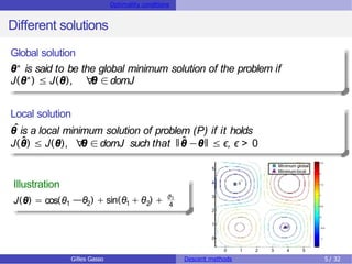
The document discusses descent methods for unconstrained optimization, focusing on the formulation of problems, optimality conditions, notions of gradients, and the existence of solutions. It explains various descent algorithms, including gradient and Newton methods, detailing the principles underlying their operation and the conditions necessary for achieving convergence to a stationary point. Key concepts such as global and local solutions, Hessian matrices, and second-order optimality conditions are also covered.

![Notions gradient Existence of a solution
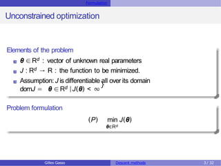
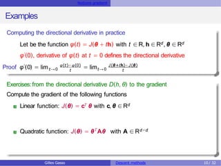
First order necessary condition
Theorem [First order condition]
Let J : Rd → R be a differential function on its domain. A vector θ0 is a
(local or global) solution of the problem (P), if it necessarily satisfies the
condition ∇J(θ0) = 0.
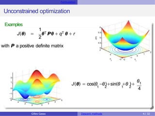
Vocabulary
Any vector θ0 that verifies ∇J(θ0) = 0 is called a stationary point or critical
point
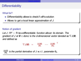
∇J(θ) ∈Rd is the gradient vector of J at θ.
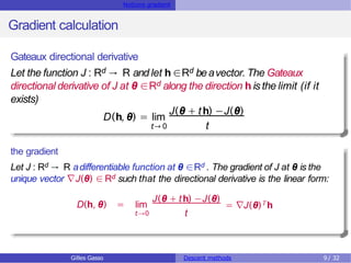
The gradient is the unique vector such that the directional derivative can be
written as:
lim
t→0
J(θ + th) −J(θ)
t
T h
= ∇J(θ) , h ∈Rd, t ∈R
Gilles Gasso Descent methods 12 / 32](https://image.slidesharecdn.com/unconstroptimeng-230327154019-fc7481f8/85/UnconstrOptim_Eng-pptx-12-320.jpg)
![Notions gradient Existence of a solution
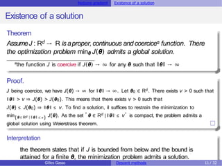
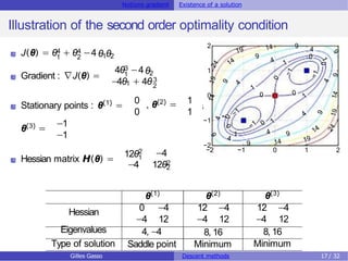
Second order optimality condition
Theorem [Second order optimality condition]
Let J : Rd → R beatwice differentiable function on its domain. If θ0 is a
minimum of J, then ∇J(θ0) = 0 and H(θ0) is a positive definite matrix.
Remarks
H is positive definite if and only if all its eigenvalues are positive
H is negative definite if and only if all its eigenvalues are negative
For θ ∈R, this condition means that the gradient of J at the minimum is
null, J′(θ) = 0 and its second derivative is positive i.e. J′′(θ) > 0
If at a stationary point θ0 H(θ0)) is negative definite, θ0 is a local
maximum of J
Gilles Gasso Descent methods 16 / 32](https://image.slidesharecdn.com/unconstroptimeng-230327154019-fc7481f8/85/UnconstrOptim_Eng-pptx-16-320.jpg)
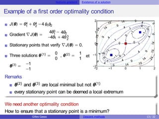
![Notions gradient Existence of a solution
Necessary and sufficient optimality condition
Theorem [2nd order sufficient condition ]
Assumethe hessian matrix H(θ0) of J(θ) at θ0 existsand is positive
definite. Assumealsothe gradient ∇J(θ0) = 0. Then θ0 is a(local or
global) minimum of problem (P).
Theorem [Sufficient and necessary optimality condition]
Let J be a convex function. Every local solution θ
ˆis a global solution θ∗.
Recall
A function J : Rd → R is convex if it verifies
J(αθ + (1−α)z) ≤ αJ(θ) + (1 −α)J(z), ∀
θ, z ∈domJ, 0 ≤ α ≤ 1
Gilles Gasso Descent methods 18 / 32](https://image.slidesharecdn.com/unconstroptimeng-230327154019-fc7481f8/85/UnconstrOptim_Eng-pptx-18-320.jpg)

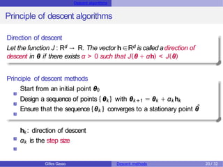
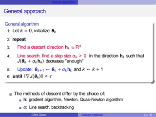
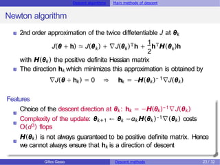
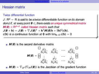
![Descent algorithms Main methods of descent
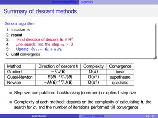
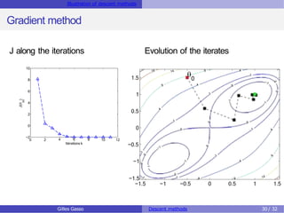
Gradient Algorithm
Theorem [descent direction and opposite direction of gradient]
Let J(θ) beadifferential function. The direction h = −∇J(θ) ∈Rd is a
descent direction.
Proof.
J being differentiable, for any t > 0 we have
J(θ + th) = J(θ) + t∇J(θ)Th + tǁhǁϵ(th). Setting h = −∇J(θ), we get
J(θ + th) −J(θ) = −tǁ∇J(θ)ǁ2 + tǁhǁϵ(th). For t small enough ϵ(th) → 0 and
so J(θ + th) −J(θ) = −tǁ∇J(θ)ǁ2 < 0. It is then a descent direction.
Characteristics of the gradient algorithm
Choice of the descent direction at θk: hk = −∇J(θk)
Complexity of the update: θk+1 ← θk −αk ∇J(θk) costs O(d)
Gilles Gasso Descent methods 22 / 32](https://image.slidesharecdn.com/unconstroptimeng-230327154019-fc7481f8/85/UnconstrOptim_Eng-pptx-22-320.jpg)