Download to read offline
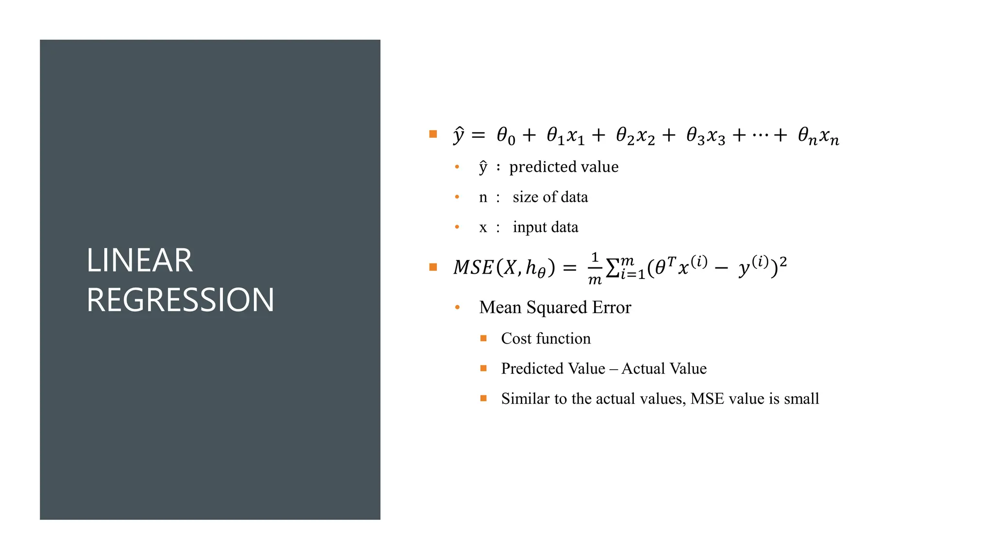
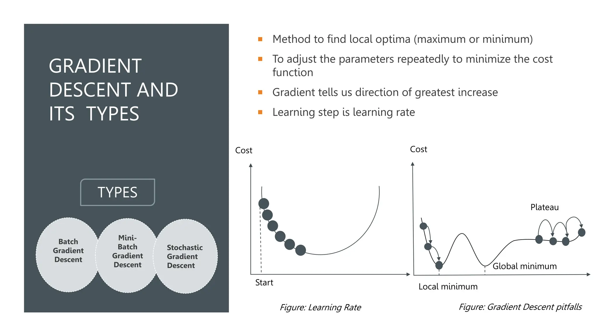
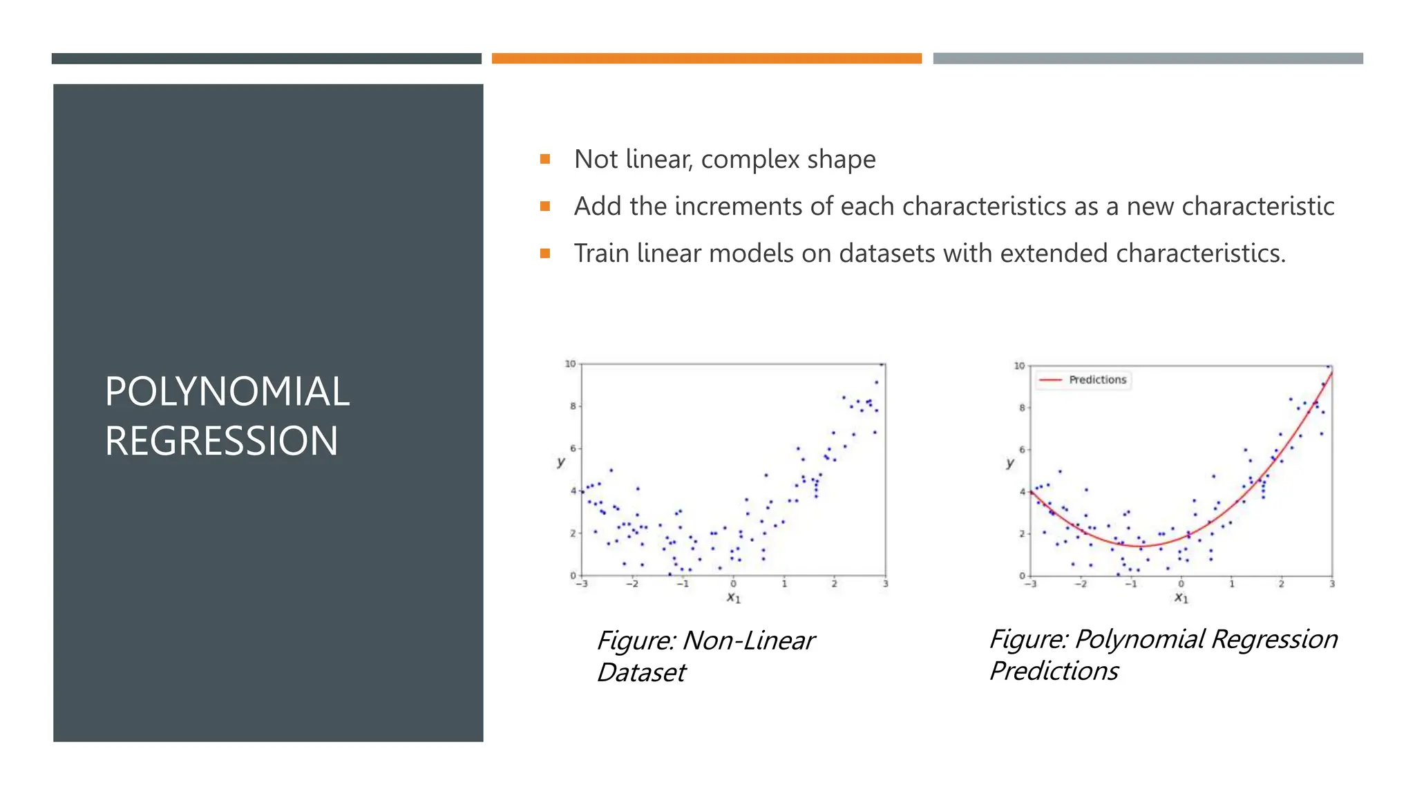
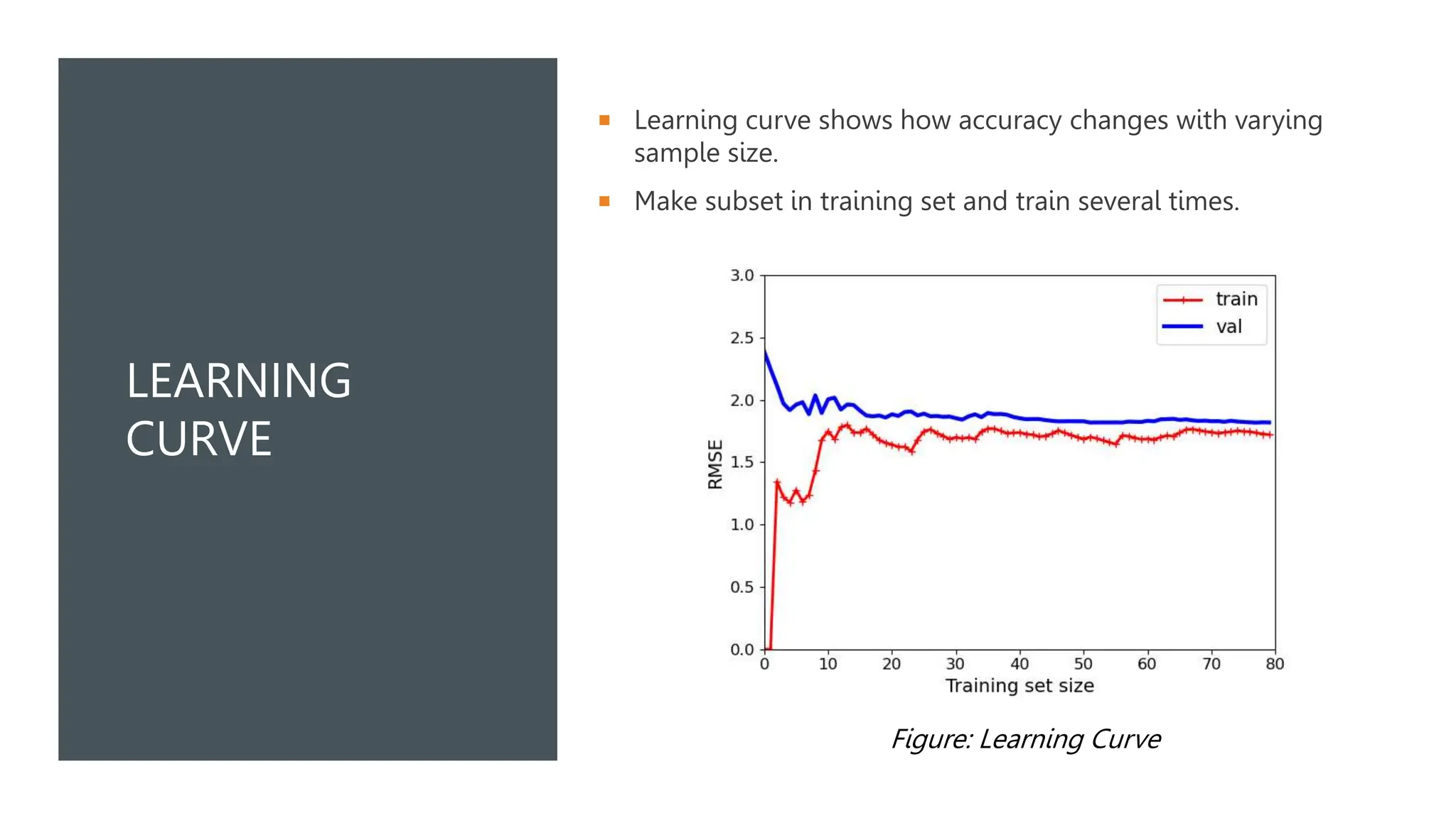
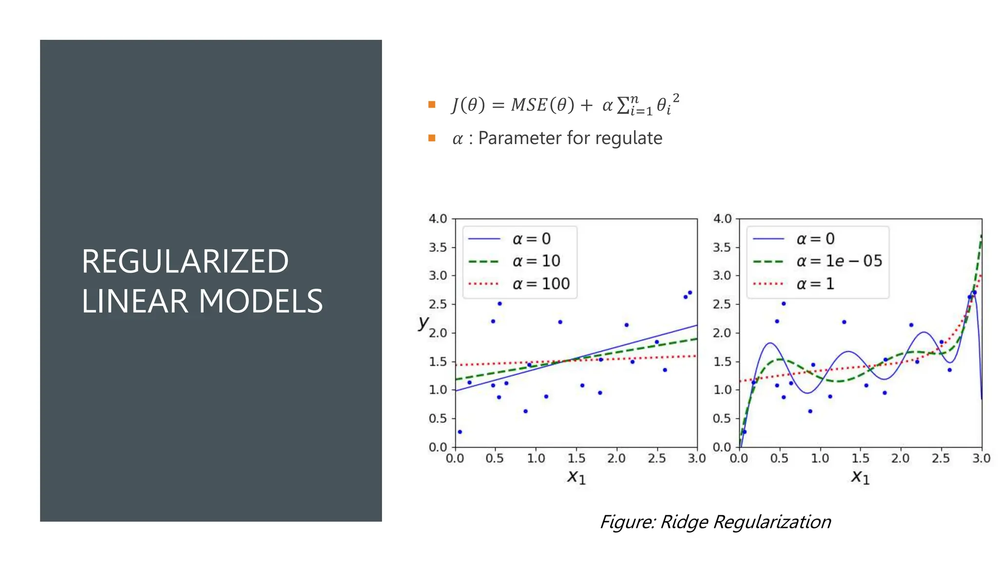
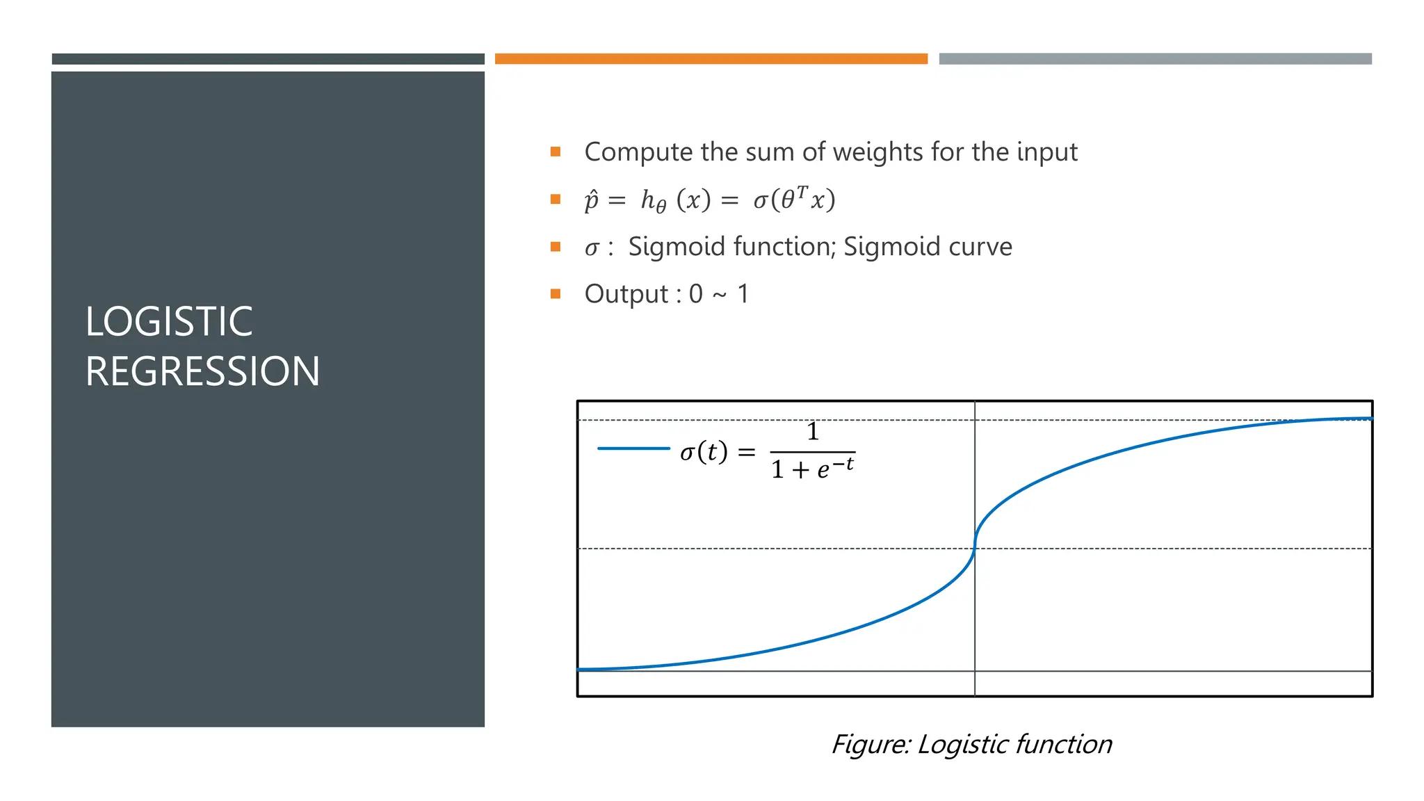


The document covers various machine learning topics including linear and polynomial regression, gradient descent, and logistic regression. It explains key concepts such as mean squared error, cost functions, and learning curves, as well as types of gradient descent methods. Regularization techniques for improving model performance are also discussed, along with the application of sigmoid functions in logistic regression.