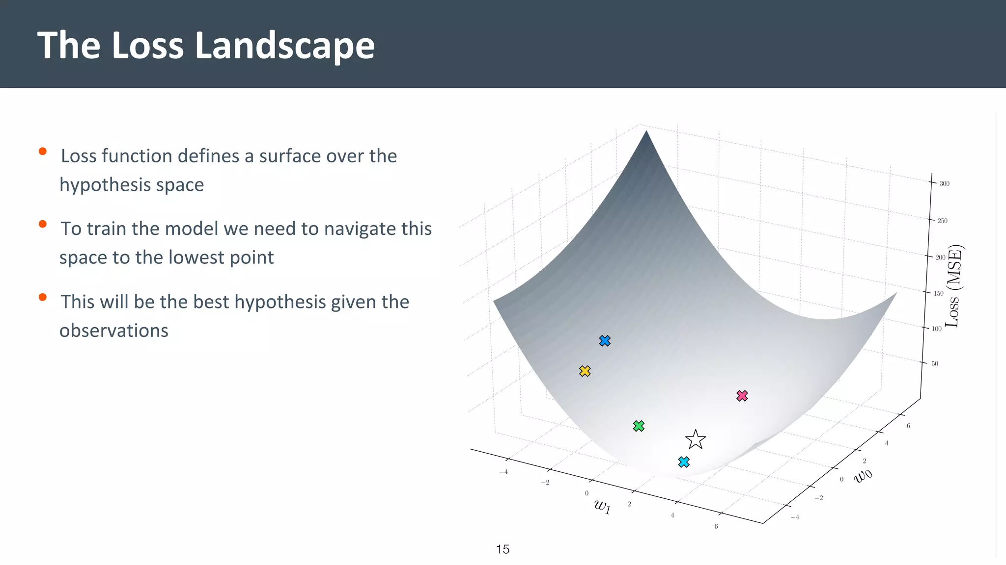
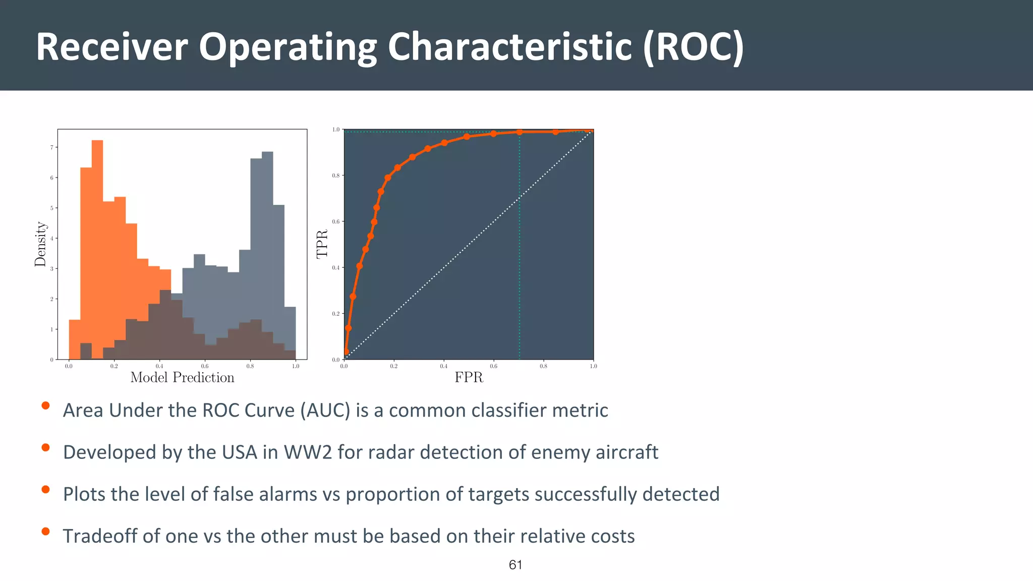
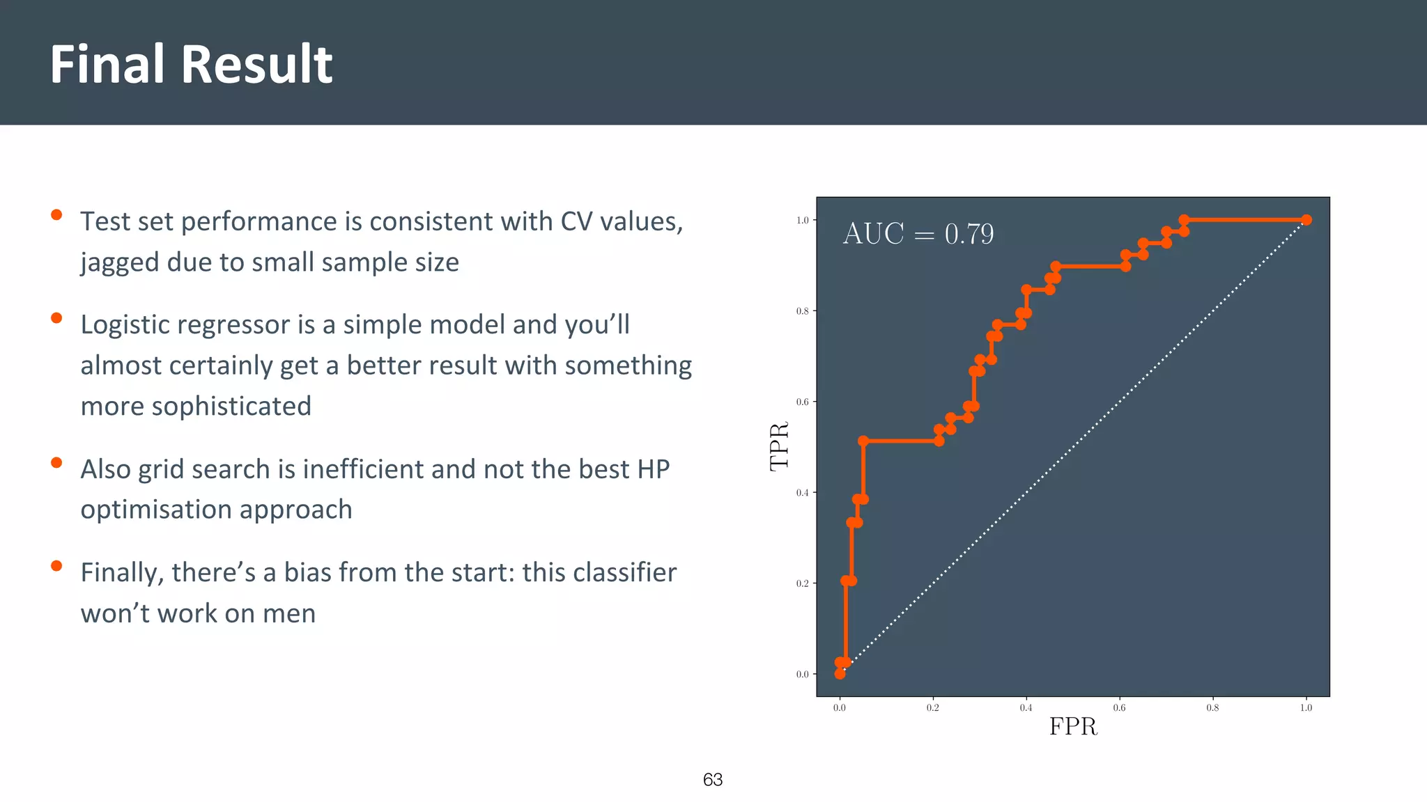
This document provides a comprehensive introduction to machine learning, covering key topics such as algorithm structures, model selection, and tuning techniques. It explains the importance of inductive bias, loss functions, and the empirical risk minimization process, illustrated with examples like linear regression and logistic regression. Additionally, it discusses practical aspects of machine learning, including data preparation, hyperparameter optimization, and the challenges of generalization in models.

1. Introduction to
Machine Learning
Liberate | Simplify | Connect www.finbourne.com
1

2. Introduction
• This talk aims to give a reasonably comprehensive
introduction to machine learning
• Covers the common structure and inner workings of
ML algorithms
• Covers how they fail, how to select and tune them
• Ties it all together at the end with a demonstration
on a real dataset
1. Learning processes
2. First Machine Learning Example
3. Empirical Risk Minimisation
4. ML Model Capacity
5. Regularisation
6. Hyperparameter tuning and model
selection
7. Example tying it all together
2

3. What is Learning
Anyway?
3

4. • Improvement at some task as measured by some
metric given some experience
• Inductive process: combine premises to reach
conclusion
• Needs some internal model that can be updated by
some optimisation process
• This model takes features (premises) and produces
predictions (conclusions)
What is Learning?
4

5. Bait Shyness in Rats
• Task: to eat without becoming unwell
• Experience: smells/tastes food. Eats a little
• Metric: level of nausea after eating
• If food makes the rat feel sick, it updates its internal
model of foods to avoid based on smell/taste
• Outcome: rat successfully learns to avoid bad food
given smell and taste features
5

6. Pigeon Superstition
• Setup: pigeon is put in a box and fed at random
• Task: to get fed
• Experience: do random action, does food appear?
• Metric: has food appeared?
• If food appears during action, update model and do
action more often
• Outcome: pigeons learn to do random things
unconnected to when they’re fed (superstitions)
6

7. What happened?
• Why did the rats succeed and the pigeons fail?
• Rats don’t avoid food if given a different unpleasant
stimulus
• Rats have an inductive bias towards associating
smells, tastes and nausea with bad food (due to
natural selection)
• Inductive bias is crucial for learning: without it
learning can’t succeed
• For a machine to be able to learn we need to
describe this learning process mathematically
7

8. How to Describe Observations
• Feature vector: values to make predictions
from
• Target: desired prediction values (optional)
such as class labels or continuous values
• Data-Generating Process: the unknown
probability distribution that feature vectors
and targets are drawn from.
• Dataset: collection of feature vectors (and
optionally) paired with target values
8

9. Features and Data: Irises
9
0 1 2 3 4 5 6 7
petal length (cm)
0.0
0.5
1.0
1.5
2.0
2.5
3.0
petalwidth(cm)
Iris Features
Setosa
Versicolor
Virginica
[1.4 0.2][0]
[1.4 0.2][0]
[1.3 0.2][0]
[1.5 0.2][0]
[1.4 0.2][0]
[6.0 2.5][2]
[5.1 1.9][2]
[5.9 2.1][2]
[5.6 1.8][2]
[5.8 2.2][2]
[4.7 1.4][1]
[4.5 1.5][1]
[4.9 1.5][1]
[4.0 1.3][1]
[4.6 1.5][1]
1 2 3 4 5 6 7
petal length (cm)
Iris Features
Setosa
Versicolor
Virginica

10. How Can Machines Learn?
• Model: takes vector of features given an internal
vector of parameters and produces a prediction
• Loss: function that takes predictions and gives a
score (lower is better by convention). Encodes our
opinion of what a good prediction is.
• Optimisation: a process that alters the model
parameters to reduce the loss and drives the
learning process.
• Inductive Bias: manifests everywhere as our
choices in the above objects
10

11. A First Example: Linear
Regressor
11

12. Problem and Dataset
• Dataset: generated from linear
relationship plus some random value that
smears the observation
• Random value is drawn from Gaussian
with mean = 0 and standard deviation = 2
• Problem: predict value of target y given
feature x
12

13. Model and Parameters
• Model is a simple linear function (a straight line): y = w0+w1x
• Has two parameters: w0 (intercept) and w1 (line gradient) that form a space
• Each point is a hypothesis about the data-generating process
• How can we evaluate a hypothesis?
13

14. The Loss
• Loss function in this case is the Mean Squared Error (MSE)
• We can choose a hypothesis by measuring the loss of a collection of hypotheses and picking the lowest
• Eyeballing a graph isn’t going to scale though…
14

15. The Loss Landscape
• Loss function defines a surface over the
hypothesis space
• To train the model we need to navigate this
space to the lowest point
• This will be the best hypothesis given the
observations
15

16. Navigation: Loss Gradients
• Gradients of the loss surface guide the
model to the minimum
• Most ML algorithms use some sort of
gradient descent in their training process
16

17. The Training Process
• Model is initialised at w=(5,-3)
• Steps down the loss landscape along the
gradient
• Step size is equal to the gradient size
multiplied by a scale factor: the learning
rate
• Stop when the gain in performance is
below threshold
17

18. Final Result
• Training has not produced the true
relationship
• Fit to the sample is good though
• Problem is that the sample is an imperfect
measurement of the data-generating
process
• Random noise has pulled the y values down
in the low x region
• We are optimising for the loss calculated
with observed data
18

19. Empirical Risk
Minimisation
19

20. Empirical vs True Loss
• ERM is a formal model of statistical learning
processes where we choose hypotheses that
minimise empirical loss (aka risk)
• Empirical loss is the loss measured with
respect to observation
• We are minimising this empirical loss, not the
true loss
• We don’t know the true loss because we
don’t know the true data-generating process
20

21. Empirical Issues
• Small samples will be sensitive to fluctuations that distort the loss surface
• Class imbalance and different feature scales can also distort this landscape in a way that will cause models
to fail to generalise
21

22. °3 °2 °1 0 1 2 3
x
0
100
200
300
400
500
Later
Decision Line
Class 0
Class 1
0
100
200
300
400
500
Now
Independent and Identically Distributed
• Non independent and identically distributed
(IID) processes will cause issues. IID is a key
assumption in many algorithms.
• Identically distributed: distribution is not
changing between sampling
• Independent: samples do not affect each
other. Are you intervening in the data
generating process by sampling it?
• Many real world distributions will change
over time: this is domain shift (aka concept
drift). Your trained algorithm will have a
shelf life.
22

23. Primer: Decision Trees
• Models can fail even if empirical loss is fine:
memorising the training data could get an
empirical loss of zero
• Decision trees are a good example of this
• DTs partition feature space to optimise loss
at each cut
• Defines a branching tree structure where the
leaves are predicted values
23

24. Generalisation Error: Variance
• This tree is an example of such a
memorisation function
• Achieves perfect loss on training set (loss =
0)
• Fails completely on new data drawn from
same distribution
• This is variance error, a type of
generalisation error (aka overfitting)
24

25. Primer: Logistic Regressor
• Model is based on Sigmoid function: outputs number between 0 and 1, given a weighted sum of features
and constant
• Inductive bias is for a linear (straight) decision boundary in feature space
25

26. Generalisation Error: Bias
• When classes are not linearly separable the algorithm fails completely
• Logistic regressor’s inductive bias is inappropriate leading to bias error (aka underfitting)
26

27. From Bias to Variance
27

28. From Bias to Variance
28

29. From Bias to Variance
29

30. From Bias to Variance
30

31. From Bias to Variance
31

32. From Bias to Variance
32

33. From Bias to Variance
33

34. From Bias to Variance
34

35. Bias-Variance Tradeoff
• Generalisation errors from
bias and variance are linked
and must be traded off each
other
• Generalisation error is
measured with holdout data:
a test set
• The underlying property
driving this trade off is model
capacity
35

36. Capacity and
Hypothesis Space
36

37. Capacity and Hypothesis Space
• A model’s capacity is linked to the size of its hypothesis
space
• If the hypotheses are too restricted the model will not be
able to describe what it sees
• Too large and the algorithm can select over-complicated
Rube-Goldberg machine solutions
• Can truncate this space (remove dimensions - e.g.
polynomial degree)
• an alternative is to introduce a penalty over the space:
regularisation terms
37

38. Regularisation
• Regularisation is a broad class of techniques for
improving ML algorithms’ generalisation
• Regularisation terms are functions of the model
parameters that are added to the loss
• These function as penalties over the hypothesis space
• Two particularly common examples based on L1 and L2
norms
38

39. L1 Term
• Manhattan distance
• AKA LASSO when used in linear regression
• Encourages sparsity where some parameters are large and others close to zero
39

40. L2 Term
• Squared Euclidean norm (normal distance)
• AKA Ridge when used in Linear Regression
• Encourages all parameters to be small as possible
40

41. Demo: Toy Data & Model with L2
• Generated from a cubic where w0 and w1 are
zero, plus gaussian noise
• Model is a cubic polynomial, but only the x2 and
x3 terms matter so the hypothesis space is 2D
• Loss is the same bowl-shaped MSE loss
• L1 is going to make the loss landscape more
“inverted pyramid”-like
41

42. Increasing Regulariser Strength
42

43. Increasing Regulariser Strength
43

44. Increasing Regulariser Strength
44

45. Increasing Regulariser Strength
45

46. Increasing Regulariser Strength
46

47. Increasing Regulariser Strength
47

48. Hyperparameters and
model selection
48

49. Hyperparameters and Model Selection
• Hyperparameters are non-learned model parameters such as regulariser
strength
• Can’t use training data to tune them because the training process will just grant
itself max capacity and overfit
• Can’t use the test data to tune them because we lose our unbiased estimate of
generalisation performance
• To select these we optimise with respect to another holdout set, typically a
subsample of the training data: a validation set
• Selecting which ML algorithm to use follows the same workflow
49

50. Hyperparameter Search Example
• Data: quadratic plus noise
• Algorithm: linear regressor with 9th-order
polynomial features and L1 regulariser
(LASSO)
• Procedure:
1. Scan along hyperparameter range
2. For each value of HP train the algorithm
3. Test on validation set
4. Pick the best one
50

51. Tuning with Validation Set
51

52. Tuning with Validation Set
• This optimisation is sensitive to
noise in the validation set
• Have experienced variance error
and in effect overfitted again
• Demonstrates why it’s so
important to not use the test set
for tuning
52

53. K-Fold Cross Validation
• K-Fold Cross Validation offers a
better approach
• Split the data into N-many folds.
Train on N-1 validate on the
holdout. Repeat over
combinations.
• Will in effect “smooth out” the
fluctuations
• Will also give us a measurement of
the variance of the model
53

54. Tuning with Cross Validation
• Idea is the same as before
• Instead of working with one train/validation
set we use combinations of the four folds
• Also repeat this 10 times, shuffling the data
before doing the CV again
• This all smooths the observed relationship
• Pick the one with the best performance
averaged over all the runs
54

55. Results Comparison
• CV has produced a final result that’s
closer to the true relation
• Test set is also noisy and isn’t going to
favour one over the other
• Ideally we gather more data, but if that’s
not possible CV offers a good way to
smooth out the statistical fluctuations
55

56. Putting it all together: a
Practical Example
56

57. Akimel O’otham (Pima) Diabetes Dataset
• Dataset gathered from the Akimel O’otham people
for diabetes study
• Native Americans as a group have a genetic
predisposition for developing type 2 diabetes
• Specifically of women with and without type 2
diabetes
• Objective is to develop a classifier that will predict
whether or not an individual has diabetes
57

58. Data Exploration and Cleaning
n_pregnancies plasma_glucoseblood_pressure skin_thickness insulin bmi pedigree_func age outcome
6 148 72 35 0 33.6 0.627 50 1
1 85 66 29 0 26.6 0.351 31 0
8 183 64 0 0 23.3 0.672 32 1
1 89 66 23 94 28.1 0.167 21 0
0 137 40 35 168 43.1 2.288 33 1
5 116 74 0 0 25.6 0.201 30 0
3 78 50 32 88 31 0.248 26 1
10 115 0 0 0 35.3 0.134 29 0
2 197 70 45 543 30.5 0.158 53 1
8 125 96 0 0 0 0.232 54 1
4 110 92 0 0 37.6 0.191 30 0
10 168 74 0 0 38 0.537 34 1
10 139 80 0 0 27.1 1.441 57 0
1 189 60 23 846 30.1 0.398 59 1
• There are zeros for features that don’t make sense. They are placeholder values for missing measurements
• For simplicity just throw these rows out. However, there are other ways of handling it
• There is a class imbalance with twice as many non-diabetic as diabetic people
58

59. Exploration: Marginal Distributions
59

60. Setup and Procedure
• ML Algorithm: SKLearn Logistic Regressor with elastic net
regularisation and balanced class weights
• Data Split: 70% train, 30% test.
• Data Preprocessing: features are mean subtracted and scaled
by their standard deviation.
• HP Search: grid search in 2D plane using 4-fold CV and AUROC
as the objective.
• Selected HP model trained on entire training set, with final
result given as a ROC curve on test data.
60

61. Receiver Operating Characteristic (ROC)
• Area Under the ROC Curve (AUC) is a common classifier metric
• Developed by the USA in WW2 for radar detection of enemy aircraft
• Plots the level of false alarms vs proportion of targets successfully detected
• Tradeoff of one vs the other must be based on their relative costs
61

62. Hyperparameter Grid Search
62

63. Final Result
• Test set performance is consistent with CV values,
jagged due to small sample size
• Logistic regressor is a simple model and you’ll
almost certainly get a better result with something
more sophisticated
• Also grid search is inefficient and not the best HP
optimisation approach
• Finally, there’s a bias from the start: this classifier
won’t work on men
63

64. What is Machine Learning?
64
• Field concerned with algorithms that improve at a task as
measured by some metric given some experience
• An empirical process where we search over many
hypotheses to find the best one (as measured by a loss
function with respect to some data)
• A biased process where our choice of inductive bias
represents the domain knowledge crucial for any algorithm
to succeed
• This bias is encoded in how we choose our algorithms, the
data we give them, how we describe what a good result is,
and in our choice of hyperparameters

65. Outlook
• Although the examples we considered are simple their usage and
optimisation is common amongst all ML algorithms
• They also set the groundwork for more complex ones:
• Decision Trees are weak learners commonly used in ensembles
(XGBoost, LightGBM) a class of techniques for fighting variance
• Logistic Regressors are the individual neurons of neural nets (Deep
Learning)
• Mapping non-linearly separable data into a space where they are
underlies kernels (Kernel Support Vector Machines, Gaussian
Processes)
65

66. Jack Wright
Jack.wright@finbourne.com
Liberate | Simplify | Connect www.finbourne.com
66