Downloaded 36 times


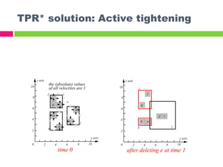
![TPR* solution: Choose path
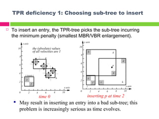
Aims at finding the best insertion path globally, namely,
among all possible paths.
Observation: We can find this path by accessing only a few
more nodes (than the TPR-tree algorithm).
20 4 6 8 10
2
4
6
8
10
x axis
y axis
c
d
a
b g
h
p
e
f
i
inserting p at time 2
Maintain a priority queue:
[(g),0], [(h),0], [(i),20]
the path expanded so far
the accumulated penalty so far](https://image.slidesharecdn.com/tprstar-tree-140621223405-phpapp02/85/Tpr-star-tree-9-320.jpg)
![TPR* solution: Choose path
20 4 6 8 10
2
4
6
8
10
x axis
y axis
c
d
a
b g
h
p
e
f
i
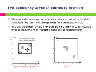
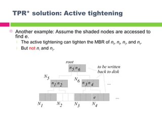
inserting p at time 2
Visit node g:
[(h),0], [(a,g),3], [(i),20],
[(b,g),32]
complete paths already
although nodes a and b are
not visited](https://image.slidesharecdn.com/tprstar-tree-140621223405-phpapp02/85/Tpr-star-tree-10-320.jpg)
![TPR* solution: Choose path
20 4 6 8 10
2
4
6
8
10
x axis
y axis
c
d
a
b g
h
p
e
f
i
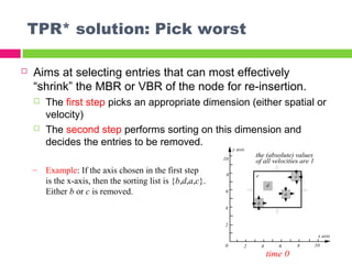
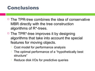
inserting p at time 2
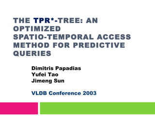
Visit node h:
[(a,g),3], [(d,h),9],
[(c,h),17], [(i),20],
[(b,g),32]
The algorithm stops now.](https://image.slidesharecdn.com/tprstar-tree-140621223405-phpapp02/85/Tpr-star-tree-11-320.jpg)

![Experiments: Settings (query and tree)
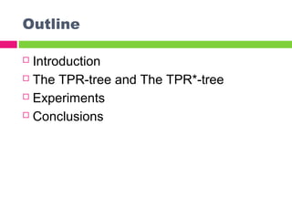
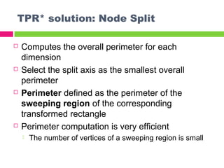
Dataset
50,000 sampled objects’ MBRs are taken from a real spatial dataset NJ
[Tiger]
each object is associated with a VBR such that on each dimension
The velocity extent is zero (i.e., the object does not change
spatial extents during its movement)
the velocity value distribution is randomed in range [0,8]
the velocity can be positive or negative with equal probability.
We compare TPR*- with TPR-trees.
Disk page size=1k bytes (node capacity=27 for both trees).
For each object update, perform a deletion followed by an insertion on each
tree.
Each predictive query is a moving rectangle, and has these
parameters:
qRlen: The length of the query’s MBR
qVlen: The length of the query’s VBR
qTlen: The number of timestamps covered.](https://image.slidesharecdn.com/tprstar-tree-140621223405-phpapp02/85/Tpr-star-tree-22-320.jpg)

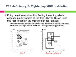
The document describes the TPR*-tree, an optimized index structure for predictive queries on moving objects in spatiotemporal databases. The TPR*-tree improves upon the Time Parameterized R-tree (TPR-tree) by addressing three deficiencies: 1) choosing a better path for insertions, 2) selecting entries that minimize node size for reinsertions, and 3) actively tightening node boundaries during deletions. Experiments showed the TPR*-tree outperformed the TPR-tree in answering predictive queries with fewer disk I/O operations.