Does early grading affect educational choices? To answer this question, I exploit a curriculum reform which postponed grade assignment in Swedish compulsory schools. The staggered implementation of the reform allows me to identify short- and long-term effects of early grading, for students with different academic ability and socioeconomic status (SES). When graded early on, high-ability students (especially if high-SES) exhibit higher grades in compulsory school, and are more likely to choose academic courses. Low-ability students react in the opposite way, with particularly negative reactions among low-SES students. High school attainment increases for high-ability low-SES students; college attainment decreases for low-ability low-SES students. None of these effects carry over to the labor market: early grading allows students to better sort into education early on. I show that the short-term effects are consistent with predictions from a learning model in which children are uncertain about academic ability, have different priors depending on SES, and use grading information to re-optimize educational choices. I find no evidence of demotivating effects for low-ability students, an alternative mechanism through which grades might affect education choices, and the main motivation behind the grading reform.

1. The Impact of Early Grading on Academic Choices:
Mechanisms and Social Implications
(Job Market Paper Draft)
Luca Facchinello
October 13, 2015
Abstract
Does early grading affect educational choices? To answer this question, I exploit a cur-
riculum reform which postponed grade assignment in Swedish compulsory schools. The
staggered implementation of the reform allows me to identify short- and long-term effects of
early grading, for students with different academic ability and socioeconomic status (SES).
When graded early on, high-ability students (especially if high-SES) exhibit higher grades in
compulsory school, and are more likely to choose academic courses. Low-ability students re-
act in the opposite way, with particularly negative reactions among low-SES students. High
school attainment increases for high-ability low-SES students; college attainment decreases
for low-ability low-SES students. None of these effects carry over to the labor market: early
grading allows students to better sort into education early on. I show that the short-term
effects are consistent with predictions from a learning model in which children are uncertain
about academic ability, have different priors depending on SES, and use grading information
to re-optimize educational choices. I find no evidence of demotivating effects for low-ability
students, an alternative mechanism through which grades might affect education choices,
and the main motivation behind the grading reform.
JEL codes: I21; I28; J13; J24
Keywords: Grades, Ability, Uncertainty, Learning, Sequential Choice, School Choice, Social
Background, Educational Attainment, Dropout, Difference in Differences
—————————————————————
Department of Economics, Stockholm School of Economics. Email: luca.facchinello@hhs.se
Acknowledgements: a special thanks to my two advisors, Erik Lindqvist and Juanna Joensen,
who provided excellent guidance and sound advice throughout the paper. I thank John
Bound, Charlie Brown, Susan Dynarski, Tore Ellingsen, Jeffrey Smith and Kevin Stange
for their valuable comments. Lastly I thank seminar participants at Stockholm School of
Economics and University of Michigan (CIERS and Economics Lunch Seminar) for their
useful feedback. I gratefully acknowledge financial support from the Swedish Foundation
for Humanities and Social Sciences (Riksbankens Jubileumsfond) grant P12-0968 enabling
the data collection for this project. The usual disclaimers apply.
1

2. Contents
Contents 2
1 Introduction 3
2 Institutional Setup 7
2.1 Data . . . . . . . . . . . . . . . . . . . . . . . . . . . . . . . . . . . . . . . . . . . 7
2.2 The Education System . . . . . . . . . . . . . . . . . . . . . . . . . . . . . . . . . 8
2.3 Grades and the Reform . . . . . . . . . . . . . . . . . . . . . . . . . . . . . . . . . 10
3 Model 12
3.1 Structure of the Model . . . . . . . . . . . . . . . . . . . . . . . . . . . . . . . . . 12
3.2 Optimal Choice . . . . . . . . . . . . . . . . . . . . . . . . . . . . . . . . . . . . . 15
4 Model’s Results 16
4.1 Effort in Compulsory School . . . . . . . . . . . . . . . . . . . . . . . . . . . . . . 17
4.2 Education . . . . . . . . . . . . . . . . . . . . . . . . . . . . . . . . . . . . . . . . 22
4.3 Summary of Results . . . . . . . . . . . . . . . . . . . . . . . . . . . . . . . . . . . 25
5 Empirics 27
5.1 Identification . . . . . . . . . . . . . . . . . . . . . . . . . . . . . . . . . . . . . . . 27
5.2 Inference . . . . . . . . . . . . . . . . . . . . . . . . . . . . . . . . . . . . . . . . . 29
5.3 Testing for Identifying Assumptions . . . . . . . . . . . . . . . . . . . . . . . . . . 29
6 Empirical Results 31
6.1 Effort in Compulsory School . . . . . . . . . . . . . . . . . . . . . . . . . . . . . . 31
6.2 Education and Income . . . . . . . . . . . . . . . . . . . . . . . . . . . . . . . . . 35
6.3 Student Welfare . . . . . . . . . . . . . . . . . . . . . . . . . . . . . . . . . . . . . 37
7 Discussion 40
8 Conclusion 42
Bibliography 44
A Numerical Model 49
A.1 Evidence on assumptions and Calibration . . . . . . . . . . . . . . . . . . . . . . . 49
A.2 Solution Method . . . . . . . . . . . . . . . . . . . . . . . . . . . . . . . . . . . . . 57
A.3 Additional Simulation Results . . . . . . . . . . . . . . . . . . . . . . . . . . . . . 64
A.4 Model and Institutional Setup . . . . . . . . . . . . . . . . . . . . . . . . . . . . . 72
B Descriptives 73
B.1 Definition of Ability and SES . . . . . . . . . . . . . . . . . . . . . . . . . . . . . 73
B.2 Education Choices, Grades and Outcomes . . . . . . . . . . . . . . . . . . . . . . 76
B.3 Treated and Control Municipalities . . . . . . . . . . . . . . . . . . . . . . . . . . 81
C Refutability Tests 90
C.1 Tests for Parallel Trends . . . . . . . . . . . . . . . . . . . . . . . . . . . . . . . . 90
C.2 Tests for Differential Response and Compositional Change . . . . . . . . . . . . . 99
2

3. 1 Introduction
While education is traditionally seen in economics as a form of investment with known
costs and returns (Becker, 1994; Ben-Porath, 1967), recent models of education choice
(e.g., Altonji, 1993) have highlighted the role of uncertainty in educational investment: the
expected return of any education choice depends ex-ante on the probability of graduation,
and thus on academic ability. When students are uncertain about ability, information, in
the form of school grades, might affect their choices.
The role of grades on education choice has been studied almost exclusively at the
college level (Stinebrickner & Stinebrickner, 2012; Zafar, 2011). Little is known about how
grades affect students at early stages of education, when children have less information
on their academic ability, and are still unconstrained by previous choices. In this paper
I investigate how assigning grades in early compulsory school affects educational choices
and attainment of Swedish students. To investigate mechanisms I compare the empirical
results to the predictions of a sequential choice learning model calibrated to the data.
The institutional setup and the data are particularly suitable to answer the research
question. In Sweden, students used to receive the first formal grades in school year 3, at
age 10. Grades were based on students’ rankings in national standardized tests, and thus
provided different information from the test scores students received during the year. In
1969 a reform allowed municipalities to postpone grade assignment to school years 6 or
7. In 1982, a second reform compelled all municipalities to postpone grade assignment to
school year 8.1 The reforms, gradually implemented over time in different municipalities,
provide a source of exogenous variation in grade assignment.
I use detailed survey and register data on cohorts born in 1967 and 1972. The 1967
cohort comprises treated students, who were living in municipalities where grading started
in middle compulsory school (school year 6), and control students, who lived in munic-
ipalities where grades were assigned starting from late compulsory school (school year
7). Students born in 1972 started receiving grades in late compulsory school (in school
year 8) in both treatment and control municipalities. If the education choices of students
in treatment and control municipalities trend in the same way over time, it is possible
to disentangle the effect of early grade assignment from pre-existing differences between
the two sets of municipalities. I provide evidence that trends in educational attainment
are the same for treatment and control municipalities, when early grades were abolished.
Moreover I show that pre-treatment differences in determinants of education appear in
1
In 2012 the reform was reversed, and grades in school year 6 were reinstated. Currently grading in school
year 4 is being discussed.
3

4. general to persist over time.
To guide the empirical analysis, I set up a model of early education choice that captures
the most important features of the institutional setup.2 In the model, ability determines
optimal effort and education choices during compulsory school: for low-ability students it
is optimal to exert low effort and enroll into vocational high school; for high-ability stu-
dents higher effort and academic education are the optimal choices. Children are uncer-
tain about their cognitive ability, and their priors reflect aggregate ability distributions:
high-SES children are on average endowed with higher ability than low-SES children.3
Grades reveal information about true ability, and allow students to re-optimize educa-
tional choices. As in the institutional setup, grades can be assigned starting from middle
or late compulsory school, while they are never assigned in early compulsory school.
The calibrated model shows that early grade assignment results in better sorting of
students into education, that is, in choices closer to first best. However, students react
differently to the ability signals, due to their different priors about ability. Low (high)
SES students who receive low (high) ability signals confirm their priors, and thus react
strongly to the information. Students who receive signals inconsistent with their priors
form imprecise posteriors, and thus their responses are weaker. When graded early on,
students with particularly low ability increase effort in compulsory school, are more likely
to choose vocational high school, and thus less likely to drop out of high school. Low-
ability students on average reduce effort in compulsory school, and are more likely to
choose vocational education paths. These responses appear to be stronger for low-SES
students, who are more sensitive to low ability signals. When graded early on, high-ability
students increase effort in late compulsory school if they are low-SES, and decrease it if
they are high-SES. All high-ability students are more likely to choose academic high
school, but only low-SES students increase college attainment as a result of early grading:
some high-SES students fail to access college due to early reductions in effort.
The model guides the empirical analysis: I present the effects of early grades for
students with different SES and academic ability. SES is based on parental education.
Ability is directly measured from cognitive ability tests administered to both cohorts in
school year 6, before grades were assigned. To investigate empirically the effects of early
grading on short-term effort, I focus on grades and course choices in late compulsory
school. Academic electives are more demanding and prepare for academic high school,
while grades increase with effort.
Results are broadly consistent with model’s predictions: when graded early on, low-
2
The model builds on the theoretical framework outlined in Altonji et al (2012)
3
Régner (2002) discusses biases about ability for low SES students in the psychology literature.
4

5. ability students, especially if low-SES, receive lower grades and are less likely to choose
academic courses in late compulsory school. High-ability students exhibit instead higher-
grades in late compulsory school, but do not revise course choices. The pattern found in
the model is thus reproduced by the data, with the difference that high-ability high-SES
students are putting more effort, instead of reducing it, as in the model.4
I consider thereafter effects of early grades on high school choices and attainment.
Contrary to model predictions, I do not observe changes in high school track choice. I
find instead an increase in high school enrollment for all students.5 Effects on educational
attainment for low-SES students are qualitatively consistent with model’s predictions.
Early grading leads to a 3 percentage points decrease in college attainment for low-ability
low-SES students, and a 6 percentage points increase in high school attainment for high-
ability low-SES students (mostly due to a reduction in dropout). Why do empirical results
for high school choices and educational attainment among high-SES students differ from
model’s predictions? I propose as an explanation that preferences for education might
attenuate the effects of early grades. My data shows that, controlling for ability, high-
SES students’ academic high school enrollment rates are 20 percentage points higher than
those of low-SES students. At the same time grade differences in late compulsory school
between high- and low-SES students are at most one fourth of a grade: SES appears thus
to strongly influence high school choices in Sweden, independently of ability.
Do education effects carry over to the labor market? I find no effects on income at
ages 33-40, and a positive effect on upward income mobility for low-ability low-SES stu-
dents, who showed the strongest reductions in school grades and educational attainment.
This suggests that early grades improved the match between early education choices and
academic ability, and reduced over-investment in education. Methodologically I confirm
the importance of evaluating education policy in the long-run: limiting the analysis to
short-term or intermediate education outcomes would have led to different conclusions.
The idea that early grades could motivate/demotivate children in compulsory school
was the main motivation behind the grading reform. I thus empirically investigate this
alternative mechanism through which grades could affect education choice. I test for effects
of early grades on student motivation and attitudes toward school. These outcomes are
measured from survey responses, in the year in which grades where assigned, and in late
compulsory school. I find overall no evidence of early grading discouraging or motivating
students, which is consistent with grades simply revealing information to the students.
4
The result can be easily reconciled with the model assuming that different college majors require different
ability levels.
5
This is due to the increase in effort during compulsory school for high-ability students. While low-ability
students reduced effort, the weakest students could have increased effort when graded early on.
5

6. I conclude that early grading leads to better allocation of ability to education. However
it increases inequality in educational attainment and reduces effort in compulsory school
for low-ability students. The final judgement on this school policy thus depends on the
objectives of the policy-maker.
Early grading has relevant effects in the Swedish education system, in which students
are explicitly sorted into academic tracks that provide access to college (a tracked educa-
tion system). To what extent do my results generalize to different setups? As knowledge
production is cumulative, early education choices constrain late choices for all students
(e.g., college preparation affects college enrollment). Assigning grades early on might thus
affect students’ education choices and attainment also in non-tracked (comprehensive) ed-
ucation systems.6
Results are consistent with the learning mechanism outlined by Stinebrickner & Stine-
brickner (2012) and Zafar (2011), who find that college students react to grading infor-
mation. Students who get lower (higher) than expected grades are more (less) likely to
drop out/switch to an easier major. As the students are in college, it is not possible to
tell whether they are learning from grades about their academic ability or their previous
preparation. In my setup grades were assigned when children were 13, so there is less con-
cern that students are learning about previous preparation rather than ability. Moreover
I investigate how grades affect students with different ability levels, and find responses
consistent with students revising their priors about ability.
My paper is also related to the grading standards literature, which stresses the role of
ability in students’ responses to grades. Becker & Rosen (1992) and Betts (1998) show
theoretically that higher grading standards encourage high ability students to put more
effort, while students below standard might be discouraged. Betts & Grogger (2003)
empirically confirm the heterogeneous effects of increasing grading standards at the high
school level, while Figlio & Lucas (2004) find that higher standards lead to positive results
on test scores, with effects that depend on the ability of the student relative to the class.
In my setup untreated students do not observe grades, but only test scores. Absent grades,
low-SES students are likely to have lower grading standards than high-SES students (for
instance because the difficulty of the tests follow class ability), so that introducing grades
should lead to positive effects for high-SES students and negative effects for low-SES
students. My results do not confirm this, and are rather consistent with students learning
about their ability from grades.
6
Early grade assignment has a bigger impact in tracked education systems because students face early
choices, and benefit more of timely information about ability. This point has not received much attention
in the tracking literature (e.g., Brunello & Checchi, 2007).
6

7. The grading reform I consider has been previously studied in economics by Sjögren
(2010) and in the educational psychology literature by Alli Klapp (2014, 2015).7 Sjögren’s
paper uses administrative data to study long-run effects (final education and income) of
the overall grading reform. She finds evidence of a positive effect of early grading on
educational attainment for girls, and a negative effect for high-SES students. Differences
in educational attainment are found also before and after the reform took place, which
casts some doubts on the robustness of the results. My paper focuses on the mechanisms
through which grades affect education choice, and is motivated by a learning model.
Results appear to be more robust, as tests for parallel trends in educational attainment
do not fail. This is likely due to the different cohorts used: Sjögren needs to assume
parallel trends over two decades, while I only need to assume parallel trends within a
5-year period.
The paper proceeds as follows. In Section 2 I describe the data, the education system,
and the grading reforms. In Section 3 I set up the sequential choice learning model that
guides the empirical analysis, and illustrate the solution of the model. Section 4 discusses
the model’s results. In Section 5 I turn to the empirical analysis, and discuss identification,
inference and robustness. Section 6 discusses empirical results, while Section 7 relates
them to the literature. Finally, Section 8 draws conclusions.
2 Institutional Setup
2.1 Data
I use survey data matched to administrative data. The surveys are part of Evaluation
Through Follow-up (ETF), a longitudinal project which surveys every 5 years represen-
tative samples of Swedish students enrolled in compulsory school. I use waves 3 and 4
of the study, corresponding to cohorts born approximately in 1967 and 1972.8 The 1967
cohort was followed form 1980, when students were in school year 6 (most students were
13 at the time). The 1972 cohort was followed from 1982, when students were in school
year 3 (most students were 10 at the time).
Each sample consists of roughly 9000 Swedish compulsory school students (10% of
the targeted population) living in 29 (out of 290) municipalities, which are the lowest
administrative division in Sweden. Whole classes were systematically sampled from mu-
nicipalities, and the same municipalities were extracted in both waves.9 The final sample
7
Klapp’s papers are descriptive regression-control studies
8
In the following I will refer to the two samples as 1967 and 1972 cohort.
9
Municipalities are drawn with stratified sampling, with strata defined by population, fraction of left-wing
7

8. is thus a repeated cross-section, and allows to use a difference in differences identification
strategy.
The survey data contains important information for my analysis. First, in school year
6, before grades were assigned, sampled students took standard intelligence tests in verbal,
logical and spatial ability. The tests are exactly the same for both cohorts, which grants
comparability of the intelligence measures over time. At the time of the tests students
were 13, a point in which IQ should have already stabilized (Cunha & Heckman, 2009).
This allows me to investigate the effects of early grades using proper measures of ability.
Second, grades and course choices in compulsory school are recored from school registers,
which allows to inspect the effect of early grading right after grades were assigned. Third,
children filled in detailed surveys in school years 6 and 10 (the first year of high school).
They were asked to evaluate their own ability, how they chose courses/high school tracks,
and how they were feeling both in the current grade and in previous stages of their
education. I use children responses about stress, anxiety, and motivation as outcomes to
understand whether early grades had motivating/demotivating effects on the children, a
main concern in the policy debate. Finally, parents were surveyed the year their children
started to be followed up. They were asked questions about children school choices and
the role of school in Swedish society. This evidence helps to understand how the choices
of parents in grading municipalities differ from those of parents living in municipalities
where the early grades were abolished.
I match to the sample high quality register data from Statistics Sweden registers. For
both cohorts I observe parental education, income and demographics. These variables
allow me to test for compositional change in the sample, and I use them as controls in the
final specification to increase precision. From the longitudinal LISA dataset I measure
educational attainment, income, and income mobility at ages 33-40 for both cohorts. This
allows me to evaluate how the short- and medium-run effects of early grading transmit to
the labor market.
2.2 The Education System
Table 1 summarizes the Swedish educational setup for the two cohorts in my sample.
Compulsory school (Grundskola) started at age 7 and lasted 9 years. It was formally di-
vided in three stages, that could also entail physically changing schools: early compulsory
school (grades 1-3), middle compulsory school (grades 4-6), and late compulsory school
voters, fraction working in the public sector and fraction of immigrants. The three biggest municipalities in
Sweden (Stockholm, Malmö, Gothenburg) are always part of the sample. Further details on the sampling
scheme can be found in Emanuelsson (1979).
8

9. (grades 7-9). Standardized end-of-the-year grades were released at the end of each educa-
tion cycle, and in every year during late compulsory school. Early grades were over time
abolished. The next section provides details about the grades and the grading reforms.
The education system was tracked. In the spring of school year 6 children had to
choose whether to take math and English at the advanced or general level in the next
school year. Academic electives provided better preparation for academic tracks in high
school, and students could switch course type over time. At the end of compulsory school,
students could enroll in either academic or vocational high school tracks. Vocational tracks
lasted two years, provided professional training, and did not allow direct access to college.
Academic high school lasted three or four years, prepared for college, and was selective.
A high grade 9 GPA and advanced math electives in compulsory school could be used as
admission requirement.
After academic high school graduation (or taking one more year of high school after
vocational school) students became eligible to apply to college. A student quota, set by
the government, limited access to college. Slots were competitively assigned to the stu-
dents with highest GPA or SweSAT (a college entry test similar to the American SAT).10
College was tuition-free, and a mix of grants and income-contingent loans allowed admit-
ted students to pay for living expenses. Higher education was thus both meritocratic and
competitive. Appendix B.2 presents detailed evidence on education choices and attain-
ment for sampled students.
Table 1: Structure of Swedish education
Compulsory school Non Compulsory school
Early and
Middle
Late
High
School
College
Age 7-12 13-15 16-19
Selection:
- HS track
- GPA or
SweSAT
Funding:
- Free tuition and
grants
- Loans for living
expenses
School Year 1-6 7-9 10-12
Grades (3), (6) (7), 8, 9 10-12
Choices -
General or
advanced
courses
Vocational
or academic
track
Selection - -
GPA and
course
choices
10
Öckert (2002) reports that around 50% of the students were rejected admission to college in the period
I study, confirming the selective nature of Swedish higher education.
9

10. 2.3 Grades and the Reform
Formal grades were assigned in compulsory school at the end of the school year. Grades
were “close to standardized”, norm-referenced, and given on 1 to 5 integer scale. They
represented the student performance in specific subjects (math, English and Swedish),
with reference to the whole student cohort.11 Given that only homework and test scores
were assigned during the school year, grades provided students with relevant information
to assess their academic ability.
The school year in which grades were first assigned was over time postponed from
school year 3, when students were 10, to school year 8, when they were 15.12 Up to
1968 grades were assigned in school years 3, 6, 7, 8 and 9. In 1969 a curriculum reform
(Curriculum Lgr 69) allowed municipal school boards to abolish “early” grades, that is,
grades in school years 3 and 6. As a substitute for the abolished grades the reform intro-
duced parent-teacher conferences, non-compulsory biannual meetings in which teachers
evaluated pupil improvement over the year. Sjögren (2010) reports that supporters of
early grade abolition were concerned about early grades harming low SES or poorly per-
forming students. The idea behind the reform was that of making the class environment
less competitive and more inclusive.
Since 1969 more and more municipalities took the chance to abolish grades in the
early school years, but the issue was contentious. Left parties (Social Democrats and
Communists) in general favored early grades abolition, while right-wing parties (Center
party and Moderate Party) leaned towards keeping the early grades (this is confirmed in
Figure B.2 on page 81). In the end the government, led by a socialist majority, chose
to abolish “early grading” in all municipalities: starting from 1982 (Curriculum Lgr 80)
end-of-the-year grades were released only starting from school year 8, when children were
15.
Figure 1 shows in a timeline how the reforms affected the two cohorts in the sample.
Half of the municipalities in the 1967 cohort sample were assigning grades in school year
6, while the rest had abolished them.13 Grade assignment in school year 3 is not recorded
in my data for this cohort, as the children were followed from school year 6. Using
information provided in Sjögren (2010), I can assume that the municipalities assigning
grades in year 6 could have been also assigning grades in year 3. However municipalities
11
Tests were corrected by the teachers. The government used the scores to determine the national grade
distribution. When assigning final grades, teachers could deviate from test scores, if they thought the
student test performance did not reflect proficiency.
12
In 2012 grades were reintroduced in school year 6, and the government is considering assigning grades
also in school year 4.
13
Figure B.3 shows in a map which sampled municipalities were assigning early grades.
10

11. 1969 1982
Final reform: no grades
allowed in school years 3
and 6
1984
Early reform: possibility
to abolish grades in
school years 3 and 6
school year 6:
1979
1981
1976
school year 3:
Cohort
1967
Cohort
1972
Cohort
1972
Cohort
1967
Figure 1: Grading reform timeline and sampled cohorts
not assigning grades in year 6 should have also abolished grades in school year 3. No
municipality in the 1972 cohort sample was assigning grades in school year 6. While the
final reform was effective the year after the children born in this cohort were in school year
3, my data reports that no grades were assigned in school year 3. Finally end-of-the-year
grades were assigned for all cohorts and municipalities in school years 8 and 9.14
In the following I emphasize the role of grades in school year 6, rather than school
year 3. First, treatment status in my analysis is based on grade assignment in school year
6. Second, grades at the age of 13 are arguably more relevant than grades at age 10, the
end of early compulsory school. At that stage, grades might be more informative of effort,
or preferences for education, rather than academic ability. Moreover, after school year
6 students had to choose whether to take math and English at the general or advanced
level, so grades in school year 6 should be more relevant for education choices.
Table 2 summarizes the grading structure. I label treatment municipalities those
municipalities that were assigning grades in school years 6 before the final reform, and
control municipalities the ones who were not assigning grades in school year 6 before the
final reform. The treatment is receiving early grades in school year 6 (and potentially 3),
14
Differently from earlier school years, they were assigned two times per year, at the end of each semester.
Details are taken from Skolverket.
11

12. Table 2: Grade assignment
1967
Cohort
1972
Cohort
Early Grading
Municipalities
(Treatment)

13. (Year 3)
Year 6
Year 7
Year 8
Year 9
Year 8
Year 9
Late Grading
Municipalities
(Control)
Year 7
Year 8
Year 9
Year 8
Year 9
which holds for students born in 1967 who lived in treatment municipalities.
3 Model
The model presented in this section investigates how early grading affects students’ educa-
tion choices and attainment when grades convey information about ability. The qualitative
predictions of the learning model are compared to the empirical results in Section 6.
3.1 Structure of the Model
The model focuses on the link between early education choices and educational attainment.
I thus model explicitly early phases of education and treat non-compulsory education and
the labor market as realizations. The structure of the model is illustrated in Figure 2.
Compulsory education is divided, as in my setup, into three periods: early compulsory
school (t1), middle compulsory school (t2), and late compulsory school (t3). In each period
student i chooses how much effort to exert: eit ∈ {1, 2, 3}. Effort choices and academic
ability (ai) determine the knowledge (kit) the student accumulates in any period:15
kit = ωt(αai + βeit−1) + δkit−1. (1)
After the end of compulsory education students can go to work (E1) and earn low wages
15
Notice that the three stages of education have different lengths in my setup: I use weights ωt to adjust
the length of each stage.
12

14. Vocational high school
Medium wage High wage (with high ability)
No high school
Low wage
Middle compulsory school:
If grades are assigned, children update priors and, potentially, revise effort choices.
Late compulsory school:
Grades are assigned. Children update priors and, potentially, revise effort and high school choices.
Academic high school
College
Early compulsory school:
No grades are assigned. Children choose effort based on their family background (SES).
Figure 2: Structure of the model
(w1). They can enroll into vocational high school (E2) and study for two years, or enter
academic high school (E3) and study for 3 years. Both high school tracks grant medium
wage (w2) upon graduation. Academic high school is the only option that gives access
to college (E4), which lasts 4 years and grants upon graduation wages that increase with
academic ability: w3 = f(ai).16 Completing higher levels of education and accessing
academic high school requires higher knowledge (and thus higher ability and effort) at
the end of period 3. Notice that knowledge is here not productive per se, as wages fully
depend on attained education and ability. This is consistent with a signaling model, where
employers are uncertain about workers’ ability, but observe attained education. Higher
education is attained in equilibrium only by high-ability workers, who fetch higher wages
in the market. The knowledge thresholds at time 3 are the following:
¯kE2
kE3
¯kE3
¯kE4
, (2)
16
As this is a stylized model, returns to education do not reflect the substantial wage heterogeneity docu-
mented in the literature (Arcidiacono, 2004; Hussey et al, 2011).
13

15. where kEj
and kEj
are respectively the entry and attainment requirements for education
level Ej. Failure to meet the thresholds results in dropout (assumed at the midpoint of
each education level), and thus in foregone earnings. Given that high school grants the
same wage independently of track, it is optimal to enter academic high school only under
the expectation to be able to complete college.17 Academic ability indeed determines
optimal education and effort choices. Low-ability students (ai ∈ {1, 2, 3}) optimally choose
vocational school, and put during compulsory school levels of effort inversely proportional
to their ability: to reach the same education level, a weaker student needs to exert higher
effort in school. The optimal education choice of high-ability students (ai ∈ {4, 5}) is
academic high school, and thus college. To attain college education they need to exert
higher effort in compulsory school.
Students are uncertain about academic ability: ˜ait ∼ ft(a). Children start compulsory
school (t1) with a prior that reflects the ability distribution of students with the same
SES: fi1(a) = f(a|SES). Low-SES students have on average lower ability than high-SES
students. Grades are unbiased ability signals, and they allow students to update their
prior about academic ability. They can be assigned in middle compulsory school, and are
always assigned in late compulsory school, before students choose high school:
gi2 = d(ai + 2) with 2 ∼ N 0, σ2
2( ) , (3)
gi3 = d(ai + 3) with 3 ∼ N 0, σ2
3( ) , (4)
where d is a function that discretizes the normal values to the scale of ability. Grades
assigned in late compulsory school are more precise than those assigned in middle compul-
sory school: σ2
2( ) σ2
3( ). This reflects the fact that more grades are assigned in the last
period of compulsory school. Table 3 makes explicit the information structure in the three
Table 3: Information structure
Early grades Late grades
fi1(a) f(a|SES) f(a|SES)
fi2(a) f(a|gi2, SES) f(a|SES)
fi3(a) f(a|gi3, gi2, SES) f(a|gi3, SES)
periods. If early grades are not assigned in period 2, students’ beliefs remain unchanged:
fi2(a) = f(a|SES). Otherwise they are updated: fi2(a) = f(a|gi2, SES). In period 3
grades are always assigned, so that fi3(a) = f(a|gi3, SES) if no grades are assigned in
17
Notice also that I do not model entry to college, and simply consider people staying out as college dropouts.
14

16. middle compulsory school, and fi3(a) = f(a|gi3, gi2, SES) with early grades. When stu-
dents update their priors about ability, they also revise their beliefs about accumulated
knowledge in any period:
˜kit =
5
j=1
P(˜ait = j) × ωt(αj + βeit−1) + δkit−1 . (5)
3.2 Optimal Choice
At any period t, students consider the different values of each education choice. They
choose the education level that gives the highest utility, and the associated optimal effort
level eE
it :
eit = arg max
eEs
it
V E1
i (eE1
it ), V E2
i,t (eE2
it ), V E3
i,t (eE3
it ) . (6)
The value of compulsory school, V 1
i , does not depend on ability, and is thus not indexed
by time. It is maximized when effort is set to the lowest level, so it is a constant: V 1
i = k.
As vocational and academic high school have access and completion requirements, values
V E2
i,t and V E3
i,t depend on students’ beliefs about ability. They are thus indexed by time,
as ˜kt
i3 changes when new information is revealed:
V E2
i,t = 3
τ=t C(eE2
iτ ) + P(˜kt
i3 ≥ ¯kE2 ) × U((L − 2) × w2) (7)
+P(˜kt
i3 ¯kE2 )U((L − 1) × w1))
V E3
i,t = 3
τ=t C(e3
iτ ) + P(˜kt
i3 ≥ ¯kE4 ) × U((L − 7) × w3(ai) + (8)
P(¯kE3 ≤ ˜kt
i3 ¯kE4 ) × U((L − 5) × w2) + P(kE3
≤ ˜kt
i3 ¯kE3 ) × U((L − 2) × w1)
P(˜kt
i3 kE3
) × P(˜kt
i3 ≥ ¯kE2 ) × U((L − 2) × w2 + P(˜kt
i3 ¯kE2 ) × U((L − 1) × w1) .
C is a convex cost function, U is a concave utility function, and L is the number of working
years.
The effect of grades
When students are assigned grades they update their priors in the direction of their true
ability level. Figures A.5 to A.9 in Appendix A.2 show priors and posterior distributions
of ability after grades are assigned. Updating can have two effects: an “income” and
a “substitution” effect. When the student realizes she has higher (lower) ability than
expected, she revises the level of knowledge accumulated upward (downward). Provided
15

17. the optimal education choice has not changed, the student will need to put less (more)
effort to reach the level of non-compulsory education she was targeting, an “income effect”:
∂eEs
it
∂˜ait
Et =Et−1
=
∂˜kt
i3
∂˜ait
×
∂eEs
it
∂˜kt
i3
≤ 0. (9)
If after observing the signal expected ability is high (low) enough to alter optimal ed-
ucational choice, the student will instead revise effort choices upward (downward), a
“substitution effect”:18
∂eEs
it
∂˜ait
Et Et−1
=
∂˜kt
i3
∂˜ait
×
∂eEs
it
∂˜kt
i3
0. (10)
4 Model’s Results
Before discussing the model’s predictions, it is important to be clear about the purpose
of the model. First, the model is meant to qualitatively assess the effect of early grades
in the specific setup I consider. I calibrate to the data the key parameters of the model,
ability distributions and education payoffs. I set thresholds for educational attainment so
that higher levels of education require both higher ability and effort. Parameters with no
direct counterpart in the data (knowledge production function, precision of grade signals,
and value function parameters) are fixed to specific values.19 Appendix A.1 contains
further details on calibration, and provides evidence on model assumptions. Second, I do
not estimate the model. While this might be an interesting direction for future research,
my aim here is to generate predictions of the effect of early grading in a learning model,
rather than fitting the data.
I solve numerically the model under three different information setups: late grade
assignment, early grade assignment and, as a benchmark, full information.20 In Table
4 I show as a reference optimal effort and education choices by ability level under full
information. The “income effect” is clear for both low- and high-ability students: for
higher levels of ability it is optimal to put less effort. The “substitution effect” appears
when ability changes from 3 to 4: students need to put higher effort early on in order to
be able to attain college education.
18
Higher education levels always require higher knowledge.
19
Results remain qualitatively the same when slightly changing the parameters. Extreme parameterizations
lead to different predictions, but are also inconsistent with the data observed.
20
Appendix A.2 presents the simulation and solution methods.
16

18. Table 4: Optimal choices under full information
ai ei1 ei2 ei3 E V E
i,1
Low-ability
1 Medium Medium Medium Vocational 106.53
2 Medium Medium Low Vocational 112.63
3 Low High Low Vocational 115.84
High-ability
4 High High Medium Academic 126.49
5 Medium High Medium Academic 155.48
4.1 Effort in Compulsory School
Figure 3 shows optimal effort choices in t1, before grades are assigned. The fact that
additional information will arrive in t2, might change effort choice before grades are re-
leased. This is not the case in the model. Under uncertainty about ability, it is always
optimal for both low- and high-SES students to keep effort at a medium level. This is
due to three reasons. First, uncertainty favors higher effort early on: putting low effort
in the beginning might actually preclude the student form entering academic high school,
and thus college. Second, even if the student learns that she is high-ability in time, she
would then need to compensate for previous low effort levels: effort cost is convex, so
this behavior would not be optimal. Finally, knowledge production is cumulative, so it is
better to exert higher effort early on, when it is more productive.
In middle compulsory school students can be assigned grades. Figure A.10 in Appendix
A.3 compares posterior distributions of ability for low and high SES students who get the
same grades in t2. While all students update priors in the right directions, updates differ by
SES. Low (high) SES students who receive low (high) grades confirm their priors, and thus
their posterior distributions have higher densities on low (high) ability levels. Students
who receive grades different from their priors, form instead posterior distributions with
higher weight on intermediate values of ability. These posteriors are thus also less precise.
Figure 4 shows the effect of early grading on effort choices in t2, by aggregate (low or
high) ability and SES. Results for each ability level, reported in Appendix A.3, are useful
to better interpret the aggregate picture, so in the following I refer to both pictures.
Early grading changes optimal behavior in middle compulsory school only for high-SES
students: students who observe signals consistent with high-ability put higher effort (see
Figure A.11). As shown in table 4, this is consistent with optimal education choice: for
high-ability students it is optimal to exert high effort in middle compulsory school, and
then reduce effort in late compulsory school. Low-SES students do not react differently
at this stage, independently of ability. Their priors are set lower, and hence posteriors
17

19. about ability are less sensitive to the high grades they observe.
In t3 all students are graded. Figure 5 shows that high-SES students with high-ability
strongly react to the additional grades, and put lower effort. Together with the reaction in
middle school, this can be overall interpreted as a negative “income effect”. High-ability
low-SES students react to early grades in the opposite way: they increase effort. Against
their priors, these students realize they are high-ability. They thus switch education and
effort choices (“a substitution effect”). Low-ability students reduce effort when graded
early on. Figure A.12 shows that the strongest reductions are found among low-SES
students. The aggregate effect for low-ability students masks a positive “income effect”
among lowest ability students. Figure A.12 shows that, when graded early on, these
students put more effort to reach the same education level they targeted (an “income
effect”). This effects is strongest among low-SES students.
18

20. 27.9 43.2 28.9
100.0
31.2 46.8 22.0
100.0
High-SES
Low-SES
Full Info
Uncertainty
Full Info
Uncertainty
Early Effort Choice by Information Regime and SES
Low Medium High
Figure 3: Early effort choice by SES and information regime
Note: The Figure plots effort distributions in early compulsory school. Since in this period no
grades are assigned, choices are the same for both low and high ability students, and can only
differ by SES. Assigning early or late grades does not change effort choices in t1.
19

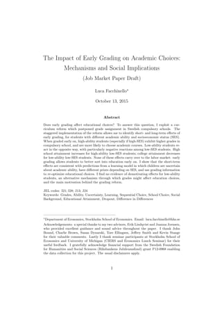
21. 100.0
100.0
100.0
54.1 45.9
100.0
100.0
High-ability
Low-ability
Full Information
Early Grades
Late Grades
Full Information
Early Grades
Late Grades
Low-SES
100.0
60.4 39.6
100.0
41.9 58.1
94.8 5.2
100.0
High-SES
Intermediate Effort Choice by Grading Regime, Ability and SES
Medium High
Figure 4: Intermediate effort choice by aggregate ability and SES for different grading
regimes
Note: The Figure plots effort distributions in middle compulsory school. Results are presented for
low-ability students, for whom it is optimal to follow an academic education path, and low-ability
students, whose optimal choice is vocational high school. SES affects students’s priors about
ability, and thus optimal choices.
20

22. 100.0
27.9 0.1 72.0
28.4 0.2 71.4
81.0 19.0
68.5 20.8 10.6
67.5 19.0 13.5
High-ability
Low-ability
Full Information
Early Grades
Late Grades
Full Information
Early Grades
Late Grades
Low-SES
100.0
17.2 21.7 61.1
19.6 0.1 80.3
87.3 12.7
69.0 12.1 18.9
66.4 12.5 21.2
High-SES
Late Effort Choice by Grading Regime, Ability and SES
Low Medium High
Figure 5: Late effort choice by aggregate ability and SES for different grading regimes
Note: The Figure plots effort distributions in late compulsory school. Results are presented for
low-ability students, for whom it is optimal to follow an academic education path, and low-ability
students, whose optimal choice is vocational high school. SES affects students’s priors about
ability, and thus optimal choices.
21

23. 4.2 Education
Figures 6 and A.13 show high school choices in the three information regimes. When
graded early on, low-ability students are less likely to choose academic education paths.
The effect is stronger for low-SES students. All high-ability students are instead more
likely to choose academic high school with early grades. Among students with high (but
not top) ability, the reaction is stronger for high-SES students.
Figures 7 and A.14 show final education distributions for the different grading setups.
The effects of early grades mirror those observed for education choice. The main difference
is that some high (but not top) ability students with high-SES fail to attain college, and
only complete academic high school. These students observed signals consistent with top
ability early on, lowered effort, and thus failed to graduate from college (see Figure A.16).
No such effect is found for low-SES students, who are actually less likely to dropout of
both high school (see Figure A.15) and college (see Figure A.16).
22

24. 100.0
28.0 72.0
28.6 71.4
100.0
89.4 10.6
86.5 13.5
High-ability
Low-ability
Full Information
Early Grades
Late Grades
Full Information
Early Grades
Late Grades
Low-SES
100.0
17.2 82.8
19.7 80.3
100.0
80.9 19.1
78.8 21.2
High-SES
High School Choice by Grading Regime, Ability and SES
Vocational Academic
Figure 6: High school choice by aggregate ability and SES for different grading regimes
Note: The Figure plots high school choice distributions. Results are presented for low-ability
students, for whom it is optimal to follow an academic education path, and low-ability students,
whose optimal choice is vocational high school. SES affects students’s priors about ability, and
thus optimal choices.
23

25. 100.0
28.0 72.0
28.6 71.4
100.0
6.3 83.1 10.6
7.7 78.8 13.4
High-ability
Low-ability
Full Information
Early Grades
Late Grades
Full Information
Early Grades
Late Grades
Low-SES
100.0
17.2 3.3 79.5
19.7 80.3
100.0
5.8 75.0 19.1
6.3 72.6 21.1
High-SES
Final Education by Grading Regime, Ability and SES
Compulsory Vocational HS Academic HS College
Figure 7: Final education by aggregate ability and SES for different grading regimes
Note: The Figure plots final education distributions. Results are presented for low-ability stu-
dents, for whom it is optimal to follow an academic education path, and low-ability students,
whose optimal choice is vocational high school. SES affects students’s priors about ability, and
thus optimal choices.
24

26. 4.3 Summary of Results
In Table 5 I summarize the effects of early grading (the treatment) on education choices,
educational attainment, and income. The effects are reported for each ability and SES
group, and are compared to the baseline scenario (late grading, in brackets).
In general early grades lead to an overall reduction in effort.21 Only high-ability low-
SES students, for whom positive “substitution effects” prevail, increase effort when graded
early on. While the mean reduction in effort is the same for all low-ability students,
effects are qualitatively different by SES. As seen before, there are weaker negative “income
effects” for high-SES students, and both positive and negative “income effects” for low-SES
students. The biggest negative “income effect” on effort is found for high-ability high-SES
students, who are the most sensitive to high grade signals.
Staying out of high school is never optimal in the model, even when students realize
they have lower ability than expected. The rational choice for these low-ability students
is to enroll into vocational school, and later dropout if they fall short of the required
preparation. This does not change with early grades, which instead have nontrivial effects
on high school track choices: all low ability-students are less likely to enroll into academic
tracks, and the opposite is true for high-ability students. Positive reactions are strongest
for high-SES students, and negative reactions are more pronounced for low-SES students.
Even if they reduced effort after observing early grades, all low-ability students benefit
of the early information, due to the different choices taken at the end of compulsory school:
dropout rates decrease, in particular for low-SES students. This translates one to one into
an increase in high school attainment. Finally, college attainment increases for high-ability
low-SES students, and slightly decreases for high-ability high-SES students.
In the long-run the effects of early grades on education translate into small increases
in lifetime income for all students, with the exception of high-ability high-SES students.
While effects on income are pretty small, most of the gains in utility are due to the early
reductions in effort, so that early grading improves on average the welfare of all students.
All in all the simulations show that assigning grades earlier leads to choices and edu-
cation outcomes more consistent with academic ability, with responses differing by SES.
Lowest ability students are more likely to increase effort when graded early on, especially
if low-SES. Low to medium ability students reduce effort in compulsory school, in partic-
ular if low-SES, but are more likely to choose vocational tracks, which they are able to
complete. High-ability low-SES students increase effort in compulsory school, are more
21
I take a weighted average of middle and late effort choices in order to provide a more complete picture
on the effects of early grades on effort choice.
25

27. likely to choose academic paths, and to attain college. For high-ability high-SES stu-
dents, “income effects” tend to prevail: these students put less effort when they observe
high grades, which leads some of them to fail to graduate from college.
Table 5: Summary of the effects of early grade assignment
Outcome: Low-ability High-ability
All Sample Low-SES High-SES Low-SES High-SES
Effort in late -0.033 -0.032 -0.032 0.009 -0.074
compulsory school [1.917] [1.550] [1.624] [2.359] [2.506]
HS Enrollment 0.000 0.000 0.000 0.000 0.000
[1.000] [1.000] [1.000] [1.000] [1.000]
Academic track -0.009 -0.029 -0.020 0.006 0.025
HS Enrollment [0.399] [0.135] [0.212] [0.714] [0.803]
HS Dropout -0.007 -0.014 -0.004 0.000 0.000
[0.044] [0.077] [0.063] [0.000] [0.000]
Attains HS 0.007 0.014 0.004 0.000 0.000
[0.956] [0.923] [0.937] [1.000] [1.000]
Attains College -0.001 0.000 0.000 0.006 -0.009
[0.304] [0.000] [0.000] [0.714] [0.803]
Income (0-1 scale) 0.001 0.002 0.001 0.002 -0.001
[0.752] [0.675] [0.675] [0.850] [0.884]
Utility 0.511 0.619 0.388 0.235 0.669
[117.007] [107.832] [107.197] [128.908] [133.171]
Values in brackets represent outcomes when only late grades are assigned. Effort is defined
on a 1-3 scale (1 is low effort). Income is a measure of lifetime income, and assumes
everybody starts working right after finishing their education or dropping out.
26

28. 5 Empirics
In this section I discuss identification of the effect of early grading on education choices. I
then briefly discuss inference in my setup, and lastly provide evidence on the identifying
assumptions.
5.1 Identification
The decision to assign early grades was taken by municipal school boards, and, as previ-
ously discussed, correlates with the political color of the municipality. Treatment assign-
ment is thus likely not random with respect to education outcomes. A simple comparison
of outcomes between grading and non-grading municipalities would pick up systematic
differences between the two sets of municipalities, and thus bias OLS.
In Appendix B.3 I test for differences in pre-treatment variables between graded and
non-graded municipalities in the 1967 cohort. Table B.7 shows that in graded munici-
palities children are less likely to be foreign born, score better in the ability tests, and
are less likely to switch classes over compulsory school. In terms of school level variables
(changes of teachers, class size, kindergarten) there are no big differences, in line with the
homogeneous nature of Swedish education. Parents in grading municipalities (Tables B.8
to B.12) are less likely to divorce and more likely to be married. They are slightly poorer,
less educated, and more likely to be employed in low-skill jobs or agriculture. However,
when asked about how they chose math and English courses, and the priorities of Swedish
education, parents give very similar answers. The only differences, the weight they put on
the role of parents in school choice and critical thinking in school, do not seem to imply a
different preference for children educational attainment. Altogether it appears that there
are some small differences in determinants of education choice between the two sets of
municipalities. The differences in parental education, generally thought to be one of the
most important determinants of education choice, seem to reflect a different structure of
the economy, rather than different preferences for education.
A simple cross-sectional comparison of outcomes for treated and untreated munici-
palities would likely lead to a negative bias, due to the pre-existing differences between
treated and control units. Given that I observe treatment and control group before and
after the final reform, when early grades were abolished, I can “control” for any persistent
difference between the two sets of municipalities. If outcomes trend in the same way in
the two municipalities (parallel trends assumption), it is possible to isolate the effect of
early grades. This situation is pictured in Figure 8: while the two sets of municipalities
exhibit differences in outcomes unrelated to grade assignment, these differences are sta-
27

29. old cohorts
1967 cohort
Final
Reform
Early
Reform
1972 cohort
Ungraded
in s.y. 6
Graded
in s.y. 6
Figure 8: Difference in differences identification strategy
ble over time. Observed outcomes for the 1967 treated cohort can be compared to the
counterfactual outcomes that would have been observed for the same set of municipalities
absent the treatment (early grades). This counterfactual is given by the trend observed
for the ungraded municipalities, assumed to be the same for treated municipalities. The
effect of early grading is represented in the picture by the white arrow. The empirical
specification that implements the difference in differences identification strategy is the
following:
Yimc = α + βasGradedm × 1967c + 1967c + Municm + ∆ Ximc + imc (11)
a∈{Low ability, High ability}; s∈{Low SES, High SES},
where i indexes the individual, m the municipality, and c the cohort. Municm is a vector
of fixed effects that captures persistent cross-sectional differences between municipalities.
1967c is a dummy that controls for the trend in outcomes. The variable Gradedm × 1967c
picks up any differences in outcomes between grading and non-grading municipalities,
that are not persistent, or the same, over time. Under the parallel trends assumption βas
represents the causal effect of early grading. Consistently with the model, the effect is
allowed to differ by ability and SES, indexed respectively by a and s in equation 11. SES
and ability are measured respectively using parental education and ability tests adminis-
tered in school year 6. 22 Notice that any determinant of the outcome that changes over
time in a different way between the two sets of municipalities will also enter βas, and thus
22
Appendix B.1 provides further details on ability and SES measures, and on the way I discretize them to
match the model.
28

30. bias the coefficient. Observable compositional change is controlled for in the regression
by adding Ximc, a vector of time varying pre-treatment controls. These covariates also
increase precision of the estimates.
5.2 Inference
Sample size is large (around 18000 observation), but the treatment, grade assignment,
varies at the municipal level. There are 29 municipalities in my sample, and half of them
are treated before the reform. I conservatively cluster standard errors at the municipal
level, rather than at the municipal − cohort level, which would result in twice as many
clusters.23 While the standard solution is to use cluster robust standard errors (Arellano,
1987; White, 1984), the number of clusters must be high for these standard errors to be
unbiased. Cameron et al (2008) show that cluster-robust standard errors are downward
biased in samples with few balanced (equally sized) clusters. They instead propose to use
Cluster Bootstrap-t methods with null hypothesis imposed, and find that these methods
yield the right p-values even with relatively few clusters (as few as 20). In a recent working
paper MacKinnon Webb (2014) confirm the good performance of the Cluster Bootstrap-
t in the realistic case in which clusters are unbalanced. The Cluster Bootstrap-t is shown
to perform well when treatment has enough variance.
My sample consists of 29 municipalities, both small and big. Treatment is given by
the interaction between belonging to the cohort born 1967 and studying in a grading
municipality, which holds for about a quarter of the sample. There are thus enough
clusters and treatment variation to believe that the Cluster Bootstrap-t should guarantee
unbiased standard errors in my analysis. So in all my specifications I bootstrap standard
errors using the method suggested by Cameron et al. (2008). I also use sample weights
to recover nationally representative estimates.
5.3 Testing for Identifying Assumptions
Difference in differences identifies the causal effect of assigning early grades under a specific
set of assumptions. The most important one, as discussed before, is the parallel trends
assumption: outcomes should trend similarly in both grading and non-grading municipal-
ities. The assumption is more credible when the treated and untreated populations are
not so different, especially in terms of “characteristics that are thought to be associated
with the dynamics of the outcome variable” (Abadie 2005). This was shown to be the case
23
This is suggested in Bertrand, Duflo, and Mullainathan (2004) for the case of panels. My final dataset
is instead a cluster-panel, so there should be less correlation between clusters over time.
29

31. above. In Appendix C.1 I use administrative data from Statistics Sweden to test whether
education and its determinants evolve in the same way in the two sets of municipalities:
all tests pass. In particular trends in education for cohorts who went through compulsory
school when all municipalities had abolished early grades (cohorts born 1969 onwards)
appear to be parallel. The evidence thus supports the main assumption underlying the
identification strategy.
A testable assumption of the identification strategy is that differences between treat-
ment and control group in determinants of the outcome should be stable over time (e.g.,
there should be no compositional change). In the same way, response rates should be the
same between treated and controls units over time (e.g., there should be no differential
attrition).24 In Appendix C.2 I test for differential attrition and compositional change
in the sample. First, there is no differential response to the student surveys and, im-
portantly, I find no differential attrition in availability of SES and ability data. Second,
it appears that the cross-sectional differences between grading non-grading municipali-
ties are broadly stable over time, but there is compositional change in specific parental
occupations and education levels. Therefore in my final specification I also control for
occupational dummies and parental education.
A further assumption in the difference in differences setup is that the treated popula-
tion should not change as a reaction to treatment assignment. In my setup this means that
the students born 1967 should not enroll into different schools to get/avoid early grades.
As catchment areas determined the compulsory school the student attended, parents had
to relocate to a different municipality if they wanted a different grading policy for their
children in compulsory school. Alternatively they could send their children to a private
school. The first scenario seems highly unlikely, while private schools were not common
in that period.
Finally it is important for identification that the treatment and control group do
not undergo different shocks over time. The presence of concurrent education reforms
would be a problem in my setup if they were implemented at the municipal level. During
the period I consider, schooling was quite centralized, with national curricula determining
most of school policies. There is thus little scope for additional policies being differentially
implemented in the two sets of municipalities. On top of that, the two cohorts I use in my
analysis received their education in a relatively stable educational system: Sweden had
already implemented the reforms of the 60s for the 9-year inclusive compulsory school,
24
Both compositional change and differential attrition can lead to biased difference in differences coefficients
(Blundell Costa Dias, 2009).
30

32. while the market-oriented school reforms of the 90s did not affect these cohorts.25
6 Empirical Results
The outcomes in the empirical analysis match those of the model. This allows me to
understand whether empirical findings are consistent with students learning about their
academic ability from grades. I thus investigate the effect of early grades on short-term
effort choices, high school choices and attainment, and, finally, educational attainment
and income. I also consider an alternative mechanism through which grades might af-
fect education choices: grades might motivate/demotivate students, and thus affect their
welfare.
I present difference in differences estimates from specification 11, which I re-parametrize
to directly get coefficients for each ability − SES cell. In all specifications I control for
ability (verbal and inductive ability normalized to the cohort-treatment level), basic de-
mographics (gender, birth year, foreign status, special education), SES (income, parental
occupation dummies, and education) and school-level variables (class size and teacher
changes). For every outcome I report the point estimate, the p-value in parentheses, and,
as a reference, the sample mean in brackets.26
There are two caveats when interpreting results. First, estimates are not very precise,
so I can not detect very small effects. Second, I test many hypotheses, which in principle
creates problems of false null rejection. Notice that the two problems go in opposite
directions, and that the multiple hypothesis testing problem is less severe than it seems:
most of the outcomes are strongly correlated, or can be considered different proxies for the
same underlying variable (e.g., grades and course choices proxy for effort choice). Keeping
this in mind, when I interpret results I focus on the overall picture rather than on single
coefficients.
6.1 Effort in Compulsory School
In Tables 6 and 7 I investigate effects of early grades on school effort. The first Table
reports effects on math and English course choices, which can be interpreted both as effort
choices (academic courses are more challenging), and as early school choices reflecting
future track selection (advanced courses are good preparation for academic high school).
The second Table reports effects on grades in late compulsory school, more clear measures
25
The reforms are described respectively by Meghir Palme (2005) and Björklund et al (2005).
26
The wild cluster bootstrap with null imposed does not yield standard errors.
31

33. of school effort.27
Low-ability students, especially those with low-SES, reacted to early grade assignment
by switching to non-academic English, which can be interpreted as a reduction in effort
(columns 2 and 3 in Table 6). The switches appear in grade 8, the first time in which
the students could respond to grades released at the end of school year 6, and persist in
school year 9.28 Switches in course choice are observed for English, but not for math. One
possible explanation is that parents and children already had feedback in math due to
the correction of exercises. At this proficiency level parents could probably test children’s
math skills more than their English proficiency.29 High-ability students did not revise
course choices when graded early on.
Low-ability low-SES students exhibit worse math performance when graded early on
(see column 2 and 3 of Table 7). High-ability high-SES students show instead higher
English and Swedish grades when they receive the early grades. One can clearly see from
the standardized Swedish test, which has more variation due to the different scale, that
all low-ability students performed worse after being assigned early grades, while high-
ability students performed better. Negative effects are stronger for low-SES students,
positive effects are instead more pronounced for the high-SES students. In the aggregate
no effect is found, as both positive and negative effects are summed up. This confirms
the importance of looking at heterogeneous effects.
The pattern found in the model is thus reproduced by the data: low (high) ability
students are putting less (more) effort, and effects are stronger for low (high) SES students.
However, high-ability high-SES students are putting more effort, rather than reducing
it, as in the model. This implies that “substitution”, rather than “income effects”, are
prevailing. This can be easily rationalized within the model, for instance assuming that
different majors require different ability levels. Then it is easy to see that these students
would react to high grades by further increasing effort.
27
This is especially true of Swedish, a subject that does not involve any choice.
28
The courses were chosen at the end of school year 6 for year 7, before final grades were released.
29
The parents of the treated students were born in the 40s: at that time English proficiency was less
widespread among parents than it is now the case in Sweden.
32

34. Table 6: Effects on course choices (school years 7-9):
Summary of difference in differences estimates
Outcome: Low-ability High-ability
All Sample Low-SES High-SES Low-SES High-SES
Advanced Math 0.00 -0.03 0.01 0.04 0.04
(school year 7) (0.94) (0.70) (0.84) (0.50) (0.47)
[0.73] [0.54] [0.72] [0.90] [0.95]
Advanced Math -0.01 -0.00 -0.04 0.02 -0.00
(school year 8) (0.80) (1.00) (0.26) (0.40) (0.94)
[0.66] [0.43] [0.64] [0.87] [0.96]
Advanced Math 0.02 0.01 -0.00 0.03 0.05
(school year 9) (0.64) (0.74) (0.97) (0.58) (0.16)
[0.57] [0.32] [0.53] [0.76] [0.90]
Advanced English 0.00 -0.03 -0.01 0.05 0.05
(school year 7) (0.90) (0.60) (0.88) (0.15) (0.21)
[0.75] [0.57] [0.76] [0.91] [0.97]
Advanced English -0.05** -0.06*** -0.07 -0.01 -0.01
(school year 8) (0.02) (0.01) (0.19) (0.48) (0.63)
[0.73] [0.53] [0.73] [0.91] [0.97]
Advanced English -0.06* -0.07** -0.08 -0.05 -0.01
(school year 9) (0.06) (0.02) (0.12) (0.14) (0.58)
[0.68] [0.46] [0.65] [0.87] [0.95]
* p 0.10, ** p 0.05, *** p 0.01
Wild Cluster Bootstrap p-values in parentheses; sample averages in brackets. All specifications
control for basic demographics, relative ability measures (standardized at the treatment-cohort
level) and parental background.
33

35. Table 7: Effects on grades (school years 8 and 9):
Summary of difference in differences estimates
Outcome: Low-ability High-ability
All Sample Low-SES High-SES Low-SES High-SES
Math Grade -0.02 -0.08* -0.04 0.05 0.07
(school year 8) (0.75) (0.07) (0.64) (0.14) (0.32)
[3.04] [2.70] [2.87] [3.35] [3.59]
Math Grade -0.11 -0.15** -0.13 -0.04 -0.06
(school year 9) (0.12) (0.02) (0.20) (0.68) (0.42)
[3.20] [2.86] [3.03] [3.54] [3.73]
English Grade 0.06 0.00 0.10 0.02 0.17***
(school year 8) (0.25) (0.98) (0.11) (0.79) (0.00)
[3.05] [2.70] [2.86] [3.37] [3.61]
English Grade 0.05 -0.03 0.12 0.05 0.16***
(school year 9) (0.21) (0.57) (0.11) (0.48) (0.00)
[3.18] [2.82] [3.05] [3.46] [3.73]
Swedish Grade 0.03 -0.04 -0.03 0.12 0.17***
(school year 8) (0.47) (0.38) (0.58) (0.13) (0.00)
[3.06] [2.64] [2.91] [3.43] [3.68]
Swedish Grade 0.06 -0.02 0.03 0.14** 0.18***
(school year 9) (0.17) (0.76) (0.64) (0.01) (0.01)
[3.17] [2.69] [3.03] [3.54] [3.86]
Swedish Test 0.18 -3.64*** -1.54** 4.49*** 6.14***
(school year 9) (0.84) (0.00) (0.01) (0.00) (0.00)
[15.84] [13.43] [13.25] [19.96] [18.51]
* p 0.10, ** p 0.05, *** p 0.01
Wild Cluster Bootstrap p-values in parentheses; sample averages in brackets. Math and
English pool together grades for advanced and general courses. All specifications control for
basic demographics, relative ability measures (standardized at the treatment-cohort level)
and parental background.
34

36. 6.2 Education and Income
In Table 8 I report effects of early grades on high school choices, educational attainment,
and income. Contrary to what the model predicts, early grades do not lead to different
high school track choices. I observe instead an increase in enrollment for all students.
While this can be surprising (on average low-ability students reduced effort in compulsory
school), it is possible that lowest ability students increased effort early on, and thus decided
to enroll into high school. This “income effect” was discussed in the model in Section 4.
When looking at educational attainment, I find an increase in high school attainment
at age 17-20 for high-ability low-SES students, mostly explained by a reduction in high
school dropout. In the long-run this effect becomes smaller and close to insignificant. In
Sweden adult education programs (Komvux) allow people to complete further education:
in the counterfactual scenario of late grading students might still have been able to finish
their high school education. Moreover, I find that low-ability low-SES students are less
likely to attain college. These effects are qualitatively consistent with model’s predictions:
a reduction in dropout due to higher effort in compulsory school, and less low-ability
students ending up with an academic education.
Why do short-run effects of early grades do not pass on to high school track choice,
and why is educational attainment not affected for high SES-students? I propose as an
explanation that preferences for education might attenuate the effects of early grades. In
Appendix B.2 I show that, controlling for ability, academic high school enrollment rates
of high-SES students are 20 percentage points higher than those of low-SES students.
At the same time grade differences in late compulsory school between high- and low-SES
students are at most 1
4th of a grade. SES appears thus to strongly influence high school
choices in Sweden, independently of ability.
While it is important to assess how early grades affect education outcomes to under-
stand mechanisms, a full evaluation of the policy requires looking at long-run outcomes.
Early grade assignment does not significantly affect income at ages 33-40, a good proxy
of lifetime income in the Sweden labor market (Börklund, 1993). This is consistent with
the theoretical model, which also generated very small effects on lifetime income. Early
grading leads instead to an increase in upward income mobility among low-ability low-SES
students, who displayed the strongest downward revisions in education choices.30 I can
thus conclude that, from the perspective of the labor market, early grades simply allowed
students to better sort by ability into education. For low-ability low-SES students this
implies a reduction of over-investment in education.
30
I consider upward mobile a student if she is 15 percentile ranks above the parents’ income percentile rank.
35

37. Table 8: Effects on high school choices, educational attainment and income:
Summary of difference in differences estimates
Outcome: Low-ability High-ability
All Sample Low-SES High-SES Low-SES High-SES
HS Enrollment 0.04** 0.03* 0.06** 0.03* 0.03**
(age 15-18) (0.02) (0.08) (0.03) (0.06) (0.03)
[0.89] [0.85] [0.92] [0.93] [0.97]
Academic HS Track 0.02 0.01 0.01 0.02 0.04
(age 15-18) (0.55) (0.82) (0.85) (0.68) (0.13)
[0.47] [0.20] [0.44] [0.59] [0.81]
HS Dropout 0.00 0.02 -0.01 -0.05** 0.02
(age 17-20) (0.98) (0.46) (0.53) (0.02) (0.34)
[0.13] [0.18] [0.12] [0.10] [0.08]
Attains HS 0.00 -0.02 0.02 0.06*** -0.01
(age 17-20) (0.79) (0.49) (0.35) (0.01) (0.82)
[0.79] [0.72] [0.83] [0.86] [0.91]
Attains HS 0.00 -0.02 0.03 0.02 -0.00
(age 33-40) (0.94) (0.19) (0.10) (0.14) (0.87)
[0.92] [0.88] [0.95] [0.96] [0.98]
College or more -0.02 -0.03* 0.02 -0.04 0.00
(age 33-40) (0.28) (0.06) (0.59) (0.23) (0.94)
[0.43] [0.22] [0.42] [0.52] [0.75]
Gross income 3.28 11.49 -3.64 -6.76 0.78
(age 33-40) (0.61) (0.21) (0.75) (0.62) (0.95)
[259.11] [223.88] [256.31] [269.89] [330.13]
↑ Income mobility 0.04** 0.08*** 0.02 0.01 0.02
(age 33-40) (0.02) (0.00) (0.54) (0.60) (0.60)
[0.34] [0.38] [0.27] [0.45] [0.28]
* p 0.10, ** p 0.05, *** p 0.01
Wild Cluster Bootstrap p-values in parentheses; sample averages in brackets. HS Enrollment is
measured at ages 16-18, HS attainment at age 40. Income is measured at ages 33-40. ↑ Income
mobility is 1 when student income is 15 ranks above family income rank. All specifications control
for basic demographics, relative ability measures (standardized at the treatment-cohort level) and
parental background.
36

38. 6.3 Student Welfare
Part of the policy debate in Sweden, and in other countries that considered early grades
abolition, revolved around the concern that grades might motivate (demotivate) students
who put high (low) effort independently of their ability, and create a competitive envi-
ronment where weak students fare worse.
While these aspects are not considered in my learning model, for illustrative clarity
it is useful to describe how such a mechanism would work in a formal model. Rather
than observing unbiased ability signals, students would observe signals that depend on
produced knowledge (of which grades are a mapping). The difference with respect to my
model is that students are not able to distinguish the ability signal from the grade itself,
which is a function of previous effort choices. This implies a failure in the updating process.
Under this model, early grades could lead to inefficient outcomes. For instance a high
(low) ability student with low (high) SES who put low (high) effort in early compulsory
school would mistakingly observe a low (high) ability signal, and consequently under-
invest (over-invest) in education.31
To validate this alternative mechanism I investigate the effects of early grading on
reported child welfare. Outcomes are taken from the student surveys. The first survey
was administered in school year 6, before final grades were assigned. It should pick
up potential effects due to the more competitive/challenging environment. The second
survey was assigned in school year 10, and asked many retrospective questions about
how children were feeling in late compulsory school, when I observe most of the effects
of early grades. Tables 9 and 10 show that, all in all, early grades did not significantly
affect student welfare.32 The only statistically significant effects are found for low-ability
low-SES students, who are less likely to report that they do well in school before getting
the grades, and also are less likely to report that they enjoyed late compulsory school
(school years 7-9). While the first finding is not negative per se, since it shows that these
students were more conscious of their school performance, the second one might be more
concerning for policy-makers. However similar outcomes pertaining to school welfare show
a 0 effect also for these students, so I am more inclined to consider the finding a spurious
effect.
31
Notice that for this to be the case grades must heavily reflect effort choices, rather than ability. This might
be true in higher tiers of education, but is not obvious in elementary school, where final grades might be
more indicative of ability rather than effort, due to the limited amount of personal effort required.
32
As explained before I cannot detect small effects, but I can state that there appears to be no major effect.
37

39. Table 9: Effects on behavior in school year 6:
Summary of difference in differences estimates
Outcome: Low-ability High-ability
All Sample Low-SES High-SES Low-SES High-SES
I do well in school -0.04 -0.07** -0.08 -0.01 0.03
(0.15) (0.02) (0.13) (0.71) (0.23)
[0.73] [0.61] [0.69] [0.84] [0.89]
Parents think I do -0.02 -0.02 -0.06 -0.03 0.03
well in school (0.27) (0.17) (0.11) (0.19) (0.11)
[0.89] [0.84] [0.86] [0.94] [0.96]
I do my best, even -0.02 -0.03 -0.03 -0.01 -0.01
if boring (0.30) (0.29) (0.16) (0.77) (0.88)
[0.71] [0.73] [0.71] [0.71] [0.67]
I want to improve -0.00 -0.01 -0.02 0.04 -0.03
in school (0.91) (0.77) (0.53) (0.36) (0.51)
[0.59] [0.71] [0.66] [0.47] [0.44]
I dislike answering -0.02 -0.03 -0.01 0.00 -0.04*
questions (0.34) (0.21) (0.79) (0.87) (0.07)
[0.16] [0.21] [0.18] [0.14] [0.10]
I learn useless stuff 0.01 0.03 0.03 -0.00 -0.01
at school (0.69) (0.33) (0.37) (0.97) (0.80)
[0.38] [0.39] [0.38] [0.40] [0.34]
I get disappointed 0.01 -0.02 0.02 0.04 0.03
if I get bad scores (0.65) (0.58) (0.33) (0.34) (0.26)
[0.68] [0.63] [0.70] [0.69] [0.75]
* p 0.10, ** p 0.05, *** p 0.01
Wild Cluster Bootstrap p-values in parentheses; sample averages in brackets. All specifications
control for basic demographics, relative ability measures (standardized at the treatment-cohort
level) and parental background.
38

40. Table 10: Effects on behavior in late compulsory school:
Summary of difference in differences estimates
Outcome: Low-ability High-ability
All Sample Low-SES High-SES Low-SES High-SES
I enjoyed grades -0.01 -0.03* -0.01 -0.01 0.01
7-9 (0.41) (0.07) (0.65) (0.69) (0.67)
[0.72] [0.71] [0.71] [0.75] [0.74]
I was worried in 0.01 -0.01 0.05 0.01 -0.00
grades 7-9 (0.79) (0.72) (0.65) (0.75) (0.98)
[0.12] [0.13] [0.10] [0.11] [0.12]
I am happy with 0.00 -0.01 0.00 0.02 0.00
grades 7-9 (0.81) (0.89) (0.86) (0.65) (0.86)
[0.75] [0.68] [0.71] [0.82] [0.85]
I got help at home -0.01 -0.01 -0.02 -0.01 0.02
in grades 7-9 (0.66) (0.52) (0.30) (0.62) (0.33)
[0.71] [0.67] [0.75] [0.68] [0.76]
I did my best even 0.01 -0.00 0.05 0.02 -0.00
if boring (0.62) (0.93) (0.14) (0.28) (1.00)
[0.47] [0.50] [0.47] [0.47] [0.45]
I did my best even -0.00 -0.01 0.04 -0.02 0.02
if hard (1.00) (0.44) (0.17) (0.26) (0.55)
[0.71] [0.71] [0.70] [0.71] [0.74]
I learned useless 0.03 0.04 0.03 0.05 0.01
stuff at school (0.19) (0.27) (0.19) (0.17) (0.84)
[0.53] [0.57] [0.52] [0.54] [0.47]
I was stressed at 0.01 0.01 0.00 0.00 0.02
school (0.65) (0.76) (0.86) (0.93) (0.39)
[0.20] [0.20] [0.22] [0.19] [0.19]
* p 0.10, ** p 0.05, *** p 0.01
Wild Cluster Bootstrap p-values in parentheses; sample averages in brackets. All specifications
control for basic demographics, relative ability measures (standardized at the treatment-cohort
level) and parental background.
39

41. 7 Discussion
In the following I assess how my results compare to previous literature on the effects
of grading information. Stinebrickner Stinebrickner (2012) study dropout behavior in
Berea college, an institution with free tuition and subsidized boarding catering to dis-
advantaged students. They find that dropout is strongly explained by students revising
downward their expectations of academic ability. Similarly Zafar (2011) finds that North-
western undergraduates revise downward their beliefs, and switch to easier majors, when
they observe grades lower than predicted. In Zafar’s paper the deviation between expected
and realized academic performance is taken as an “information metric” that identifies new
information about students’ “own unobserved academic ability.” In fact this information
might reflect, as explicitly recognized in Stinebrickner’s paper, college preparedness rather
than academic ability. Due to the college setup, in both studies it is not possible to deter-
mine whether the updates are on academic ability or the stock of knowledge accumulated.
While both problems signal the need for better selection into college, from the policy
perspective they have quite different implications.33 The results of my paper are in line
with the learning mechanism outlined by Stinebrickner Stinebrickner (2012) and Zafar
(2011) at the college level. In particular, the responses I find along the ability distribution
are consistent with students revising their priors about ability. Moreover, in my setup
grades were assigned when children were 13 years old, so there is less concern that the
update is on previous preparation, rather than ability. My paper shows both theoretically
and empirically that the reaction to grades differs by SES. In the above-mentioned two
papers there is no variation in SES, as sampled students are either low-SES (Berea college)
or high-SES (Northwestern undergraduate students).
My paper is also related to the grading standards literature, which stresses the role of
ability in students’ responses to grades. Becker Rosen (1992) and Betts (1998) show
theoretically that higher grading standards encourage high ability students to put more
effort, while students below standard might be discouraged. Betts Grogger (2003)
empirically confirm the heterogeneous effects of increasing grading standard at the high
school level, while Figlio Lucas (2004) find that higher standards lead to positive re-
sults on test scores, with effects that depend on the ability of the student relative to the
class. In my setup untreated students do not observe grades, but only test scores. Ab-
sent grades, low-SES students are likely to have lower grading standards than high-SES
students (for instance because the difficulty of the tests follow class ability). Introducing
33
Failure in evaluating own ability calls for a revision of grading information. Failure in college preparation
requires to revise the curricula in earlier education tiers.
40

42. grades should thus lead to positive effects for high-SES students and negative effects for
low-SES students. My results do not confirm this, and are rather consistent with students
learning about their ability from grades.
The grading reform I analyze has been previously studied by Sjögren (2010), who uses
administrative data to study long-run effects (final education and income) of the overall
reform using difference in differences. She finds evidence of a positive effect of early
grading on educational attainment for girls, and a negative effect for high-SES students.
Differences in educational attainment are found also before and after the reform took
place, which casts some doubts on the robustness of the results. My paper focuses on the
mechanisms through which grades affect education choice: the theoretical model I develop
shows that average treatment effects could mask substantial heterogeneity in the response
to grades, which suggests conditioning the analysis at least by ability. I do not find any
negative effect of early grades for high-SES students, while I do not study effects by gender,
as this would exacerbate the multiple hypothesis testing problem. Results appear to be
more robust, as trends in educational attainment for treated and control municipalities
appear to be parallel in the refutability tests. This is likely due to the different cohorts
used: Sjögren’s sample comprises twenty cohorts, so she needs to assume parallel trends
over two decades. My sample uses cohorts who studied just before and after the final
reform. I only need to assume that trends between the two sets of municipalities are the
same within a 5-year window, which I show to be the case.
41

43. 8 Conclusion
In this paper I investigate the effect of early grades on students’ education choices and at-
tainment. I exploit the staggered implementation of a curriculum reform, which postponed
grade assignment in Swedish compulsory schools, to estimate both short- and long-run
effects of early grading. To investigate mechanisms I compare empirical results to the
predictions of a sequential choice learning model based on the setup.
In the model children are uncertain about academic ability, and their priors differ by
socioeconomic status (SES). Grades are ability signals that allow children to re-optimize
educational choices. The calibrated model shows that early grading results into choices
closer to first best for all students: low-ability students reduce effort in compulsory school
and are more likely to choose vocational high school. High-ability students increase effort
in school and are more likely to choose academic education paths. Stronger responses are
found for students who observe information consistent with their priors, so that effects
differ by SES.
The empirical results of my analysis are in line with the theoretical predictions for effort
choices in late compulsory school. When graded early on, low-ability low-SES students
are more likely to get lower grades and switch to easier courses in compulsory school
than high-SES students with similar levels of ability. High-ability students, especially if
high-SES, are more likely to get higher grades in late compulsory school when graded
early on. Contrary to what the model predicts, early grades do not affect high school
track choices and educational attainment for high-SES students. In line with model’s
predictions, I find that high school attainment increases by 6 pp for high-ability low-SES
students, while college attainment decreases by 3 pp for low-ability low-SES students.
What explains the differences between model predictions and empirical findings at the
high school level? The data suggests that SES strongly influences high school choices in
Sweden, independently of ability. This might attenuate the effects of early grades. None
of the effects found on education carry over to the labor market. In particular I find
no effects on lifetime income, measured at ages 33-40. This suggests that early grading
information simply improved the match between early education choices and ability, and
reduced over-investment in education. Finally I find no evidence of demotivating effects
for low-SES students, one of the main concerns that motivated the grading reforms.
The key economic implication of my results is that students are uncertain about their
ability in early stages of education, when I show that grades affect their choices. This
contrasts with the workhorse models of education choice (Becker, 1994; Ben-Porath, 1967),
that assume complete information and thus no ex-ante uncertainty in the returns to non-
42

44. compulsory education. From the policy point of view, I establish that early grading
leads to a more efficient allocation of education, but increases inequality in educational
attainment and reduces effort in compulsory school for low-ability students. Whether early
grading is a desirable policy depends thus on the objective function of the policy-maker.
With regard to future research directions, it is possible to expand the scope of the
analysis by looking at further sources of heterogeneity, which relate to different mecha-
nisms. First, as whole classes are sampled in my data, I can look at differential effects
of grading depending on relative ability. If students judge ability against their immediate
peers, average ability students in high-ability (low-ability) classes might react positively
(negatively) to early grades. Second, average ability students might get more information
out of grades, as it is less likely that they get top or bottom scores in homework and
tests.34 Third, there could be different responses to grading information along the gen-
der dimension, as boys are found to generally be more overconfident than girls in ability
(Bertrand, 2011). Before exploring these additional sources of heterogeneity it is how-
ever important to correct standard errors for multiple hypothesis testing. This requires
some additional work, as standard errors are already bootstrapped to deal with the small
number of clusters.
Lastly, it is worthy to investigate theoretically alternative mechanisms through which
grades affect education choices, including the ones outlined above. For instance what
happens when ability signals reflect knowledge rather than ability? This can be the case
if parents and students are not able to distinguish the ability component of the grade
from previous effort choices. I argue this is a plausible mechanism when parents do not
observe children’s effort, but do observe the final grades.
34
Relatedly, Stange (2012) reports that the students for whom college grades, and the option to dropout in
college, have the highest value, are moderate ability students, who have the strongest uncertainty about
finishing college.
43

45. Bibliography
[1] Abadie Alberto, 2005. Semiparametric Difference-in-Differences Estimators, Re-
view of Economic Studies, Oxford University Press, vol. 72(1), pages 1-19.
[2] Altonji Joseph G, 1993. The Demand for and Return to Education When Education
Outcomes Are Uncertain, Journal of Labor Economics, University of Chicago Press,
vol. 11(1), pages 48-83, January.
[3] Altonji Joseph G. Blom Erica Meghir Costas, 2012. Heterogeneity in Human
Capital Investments: High School Curriculum, College Major, and Careers, NBER
Working Papers 17985, National Bureau of Economic Research, Inc.
[4] Angrist Joshua D. Pischke Jörn-Steffen. Mostly harmless econometrics: An em-
piricist’s companion, Princeton university press, 2008.
[5] Arcidiacono Peter, 2004. Ability Sorting and the Returns to College Major, Journal
of Econometrics, Elsevier, vol. 121(1-2), pages 343-375.
[6] Arellano Manuel, 1987 Computing Robust Standard Errors for Within-Group Esti-
mators, Oxford Bulletin of Economics and Statistics 49, 431–434.
[7] Azmat Ghazala Iriberri Nagore, 2010. The Importance of Relative Performance
Feedback Information: Evidence from a Natural Experiment using High School Stu-
dents, Working Papers 444, Barcelona Graduate School of Economics.
[8] Bandiera Oriana Larcinese Valentino Rasul Imran, 2008. Blissful ignorance?
Evidence from a natural experiment on the effect of individual feedback on perfor-
mance, mimeo.
[9] Basit Zafar, 2011. How Do College Students Form Expectations?, Journal of Labor
Economics, University of Chicago Press, vol. 29(2), pages 301 - 348.
[10] Becker Gary S., 1994. Human Capital: A Theoretical and Empirical Analysis with
Special Reference to Education, 3rd Edition, NBER Books, National Bureau of
Economic Research, Inc, number beck94-1, August.
[11] Ben-Porath Yoram, 1967. The Production of Human Capital and the Life Cycle of
Earnings, Journal of Political Economy, University of Chicago Press, vol. 75, pages
352.
44

46. [12] Betts Julian R, 1998. The Impact of Educational Standards on the Level and Distri-
bution of Earnings, American Economic Review, American Economic Association,
vol. 88(1), pages 266-75, March.
[13] Betts Julian R. Grogger Jeff, 2003. The impact of grading standards on stu-
dent achievement, educational attainment, and entry-level earnings, Economics of
Education Review, Elsevier, vol. 22(4), pages 343-352, August.
[14] Becker W. Rosen S., 1990. The Learning Effect Of Assessment And Evaluation
In High School, University of Chicago - Economics Research Center 90-7, Chicago
- Economics Research Center.
[15] Bertrand Marianne, 2011. New Perspectives on Gender, Handbook of Labor Eco-
nomics, Elsevier.
[16] Bertrand Marianne Duflo Esther Mullainathan Sendhil, 2004. How Much
Should We Trust Differences-in-Differences Estimates?, The Quarterly Journal of
Economics, MIT Press, vol. 119(1), pages 249-275, February.
[17] Blundell Richard Costa Dias Monica, 2009. Alternative Approaches to Evaluation
in Empirical Microeconomics, Journal of Human Resources, University of Wisconsin
Press, vol. 44(3).
[18] Börklund Anders, 1993. A Comparison between Actual Distributions of Annual
and Lifetime Income: Sweden 1951-89, Review of Income and Wealth, International
Association for Research in Income and Wealth, vol. 39(4), pages 377-86, December.
[19] Björklund Anders Clark Melissa A. Edin Per-Anders Fredriksson Peter
Krueger Alan B., 2005. The market comes to education in Sweden: an evaluation
of Sweden’s surprising school reforms, Russell Sage Foundation Publications.
[20] Borghans Lex Lee Duckworth Angela Heckman James J. Ter Weel Bas, 2008.
The Economics and Psychology of Personality Traits, Journal of Human Resources,
University of Wisconsin Press, vol. 43(4).
[21] Borghans Lex Meijers Huub Weel Bas Ter, 2008. The Role Of Noncognitive
Skills In Explaining Cognitive Test Scores, Economic Inquiry, Western Economic
Association International, vol. 46(1), pages 2-12, 01.
45

47. [22] Brunello Giorgio Checchi Daniele, 2007. Does school tracking affect equality of
opportunity? New international evidence, Economic Policy, CEPR;CES;MSH, vol.
22, pages 781-861, October.
[23] Chetty Raj Friedman N. John Rockoff E. Jonah, 2014. Measuring the Impacts
of Teachers II: Teacher Value-Added and Student Outcomes in Adulthood, Ameri-
can Economic Review, American Economic Association, vol. 104(9), pages 2633-79,
September.
[24] Colin Cameron Jonah B. Gelbach Douglas L. Miller, 2008. Bootstrap-Based
Improvements for Inference with Clustered Errors, The Review of Economics and
Statistics, MIT Press, vol. 90(3), pages 414-427, August.
[25] Cunha Flavio Heckman James, 2007. The Technology of Skill Formation, Ameri-
can Economic Review, American Economic Association, vol. 97(2), pages 31-47, May.
[26] Cunha Flavio Heckman James, 2009. The Economics and Psychology of Inequality
and Human Development, Journal of the European Economic Association, MIT
Press, vol. 7(2-3), pages 320-364, 04-05.
[27] Emanuelson Ingemar, 1979. Utvärdering genom uppföljning av elever - Ett nytt
Individualstatistikproject, Stockholm School of Teacher Education, Report 11-1979.
[28] Figlio David N. Lucas Maurice E., 2004. Do high grading standards affect student
performance?, Journal of Public Economics, Elsevier, vol. 88(9-10), pages 1815-1834,
August.
[29] Härnqvist Kjell, 1994a. Den sociala selektionen till gymnasieskola och högskola,
Rapport 1994:10, Göteborgs universitet, Institutionen för pedagogik.
[30] Härnqvist Kjell, 1998. A longitudinal program for studying education and career
development, Report 1998: 01, Göteborgs universitet, Institutionen för pedagogik
(1998).
[31] Hoxby Caroline, 2011. Program Report, NBER Economics of Education Program,
Issue 1, NBER Reporter.
[32] Jalava Nina Joensen Schrøter Juanna Pellas Elin, 2015. Grades and rank: Im-
pacts of non-financial incentives on test performance, Journal of Economic Behavior
Organization, Elsevier, vol. 115(C), pages 161-196.
46

48. [33] Hussey J. Andrew Swinton H. Omari, 2011. Estimating the Ex Ante Expected
Returns to College, American Economic Review, American Economic Association,
vol. 101(3), pages 598-602, May.
[34] Klapp Alli Cliffordson Christina Gustafsson Jan-Eric. The effect of being graded
on later achievement: Evidence from 13-year olds in Swedish compulsory school,
Educational Psychology ahead-of-print (2014): 1-19.
[35] Klapp Alli. Does grading affect educational attainment? A longitudinal study,
Assessment in Education: Principles, Policy Practice ahead-of-print (2015): 1-22.
[36] Kolenikov Stanislav Angeles Gustavo, 2005. On reuse of clusters in repeated
studies,” presented at the American Statistical Association, Minneapolis, MN.
[37] Lechner Michael, 2011. The Estimation of Causal Effects by Difference-in-Difference
Methods, Foundations and Trends in Econometrics, now publishers, vol. 4(3), pages
165-224, November.
[38] Lindqvist, Erik Roine Vestman, The Labor Market Returns to Cognitive and
Noncognitive Ability: Evidence from the Swedish Enlistment, American Economic
Journal: Applied Economics 3.1 (2011): 101-28.
[39] MacKinnon James G. Matthew D. Webb, 2014. Wild Bootstrap Inference for
Wildly Different Cluster Sizes, Working Papers 1314, Queen’s University, Depart-
ment of Economics.
[40] Meghir Costas Palme Mårten, 2005. Educational Reform, Ability, and Family
Background, American Economic Review, American Economic Association, vol.
95(1), pages 414-424, March.
[41] Mora Ricardo Reggio Iliana, 2012. Treatment effect identification using alternative
parallel assumptions, Economics Working Papers we1233, Universidad Carlos III,
Departamento de Economía.
[42] Öckert, Björn, 2002. Do university enrollment constraints affect education and earn-
ings?, Working Paper Series 2002:16, IFAU - Institute for Evaluation of Labour
Market and Education Policy.
[43] Öckert, Björn, 2010. What’s the value of an acceptance letter? Using admissions
data to estimate the return to college, Economics of Education Review, Elsevier,
vol. 29(4), pages 504-516, August.
47