The formation density log chapter 13

Petrophysics MSc Course Notes Formation Density Log
Dr. Paul Glover Page 121
13. THE FORMATION DENSITY LOG
13.1 Introduction
The formation density log measures the bulk density of the formation. Its main use is to derive a value
for the total porosity of the formation. It s also useful in the detection of gas-bearing formations and in
the recognition of evaporites.
The formation density tools are induced radiation tools. They bombard the formation with radiation
and measure how much radiation returns to a sensor.
13.2 Theory
The tool consists of:
• A radioactive source. This is usually caesium-137 or cobalt-60, and emits gamma rays of
medium energy (in the range 0.2 – 2 MeV). For example, caesium-137 emits gamma rays with a
energy of 0.662 MeV.
• A short range detector. This detector is very similar to the detectors used in the natural gamma
ray tools, and is placed 7 inches from the source.
• A long range detector. This detector is identical to the short range detector, and is placed 16
inches from the source.
The gamma rays enter the formation and undergo compton scattering by interaction with the electrons
in the atoms composing the formation, as described in Section 9.3. Compton scattering reduces the
energy of the gamma rays in a step-wise manner, and scatters the gamma rays in all directions. When
the energy of the gamma rays is less than 0.5 MeV they may undergo photo-electric absorption by
interaction with the atomic electrons. The flux of gamma rays that reach each of the two detectors is
therefore attenuated by the formation, and the amount of attenuation is dependent upon the density of
electrons in the formation.
• A formation with a high bulk density, has a high number density of electrons. It attenuates the
gamma rays significantly, and hence a low gamma ray count rate is recorded at the sensors.
• A formation with a low bulk density, has a low number density of electrons. It attenuates the
gamma rays less than a high density formation, and hence a higher gamma ray count rate is
recorded at the sensors.
The density of electrons in a formation is described by a parameter called the electron number density,
ne. For a pure substance, number density is directly related to bulk density, and we can derive the
relationship in the following way.
• The number of atoms in one mole of a material is defined as equal to Avagadro’s number N
(N≈6.02×1023
).
• The number of electrons in a mole of a material is therefore equal to NZ, where Z is the atomic
number (i.e., the number of protons, and therefore electrons per atom).

• Since the atomic mass number A is the weight of one mole of a substance, the number of electrons
per gram is equal to NZ/A.
• However, we want the number of electrons per unit volume, and we can obtain this from the
number of electrons per gram by multiplying by the bulk density of the substance, ρb. Hence, the
electron number density is
(13.1)
where: ne = the number density of electrons in the substance (electrons/cm3
)
N = Avagadro’s number (≈6.02×1023
)
Z = Atomic number (no units)
A = Atomic weight (g/mole)
ρb = the bulk density of the material (g/cm3
).
Thus, the gamma count rate depends upon the electron number density, which is related to the bulk
density of a substance by Eq. (13.1). The bulk density of a rock depends upon the solid minerals of
which it is composed, its porosity, and the density of the fluids filling that porosity. Hence, the
formation density tool is useful in the determination of porosity, the detection of low density fluids
(gasses) in the pores, and as an aid in lithological identification.
13.3 Operation
A radiation emitter and one detector are all that is necessary for a simple measurement. The early tools
had only one detector, which was pressed against the borehole wall by a spring-loaded arm.
Unfortunately, this type of tool was extremely inaccurate because it was unable to compensate for
mudcake of varying thicknesses and densities through which the gamma rays have to pass if a
measurement of the true formation is to be achieved.
All the newer tools have two detectors to help compensate for the mudcake problem. The method of
compensation is described in subsequent sections. The newer two detector tools are called
compensated formation density logs, an example of which is Schlumberger’s FDC (formation density
compensated) tool.
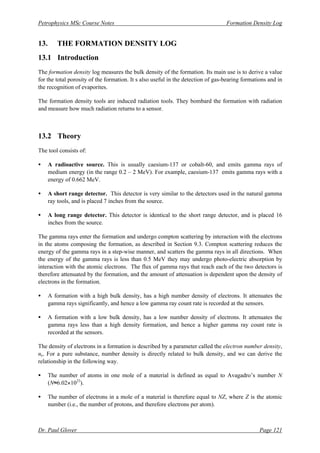
Compensated formation density tools have one focussed (collimated) radiation source, one short
spacing detector at 7 inches from the source, and one long spacing detector 16 inches from the source
(Fig. 13.1). The source and both detectors are heavily shielded (collimated) to ensure that the radiation
only goes into the mudcake and formation, and that detected gamma rays only come from the mudcake
or formation. The leading edge of the shield is fashioned into a plough which removes part of the
mudcake as the tool is pulled up the well. The tool is pressed against one side of the borehole using a
servo-operated arm with a force of 800 pounds force. Under this pressure and the pulling power of the
wireline winch the plough can make a deep impression in the mudcake. The large eccentering force
also means that there is much wear of the surface of the tool that is pressed against the borehole wall.
The heavy shielding also doubles as a skid and a wear plate that protects the source and detectors and
can be replaced easily and cheaply when worn down.
b
e
A
Z
N
n ρ
=

Figure 13.1 Schematic diagram of a formation density tool.
The operation of this tool depends upon the detection of gamma rays that have been supplied to the
formation by the source on the tool and have undergone scattering. Clearly the natural gamma rays
from the formation confuses the measurement. A background gamma ray count is therefore carried out
so that the gamma rays coming from the formation can be removed from the measurement.
Note in Fig. 13.1 that for the short spacing detector over 80% of its signal comes from within 5 cm of
the borehole wall, which is commonly mainly mudcake. About 80% of the long spacing signal comes
from within 10 cm of the borehole wall. Therefore the tool has a shallow depth of investigation. We
wish to remove the mudcake signal from the measurement, and the procedure to do this is described in
Section 13.4. When the mudcake compensation has been carried out, one can see from Fig. 13.1 that
the depth of investigation has been improved, and less signal comes from the first 5 cm region.
13.4 Mudcake Compensation
Gamma rays detected by the short spacing detector have penetrated only a short way into the mudcake
and formation before being scattered back to the detector. Readings from the short spacing detector are
therefore a measure of attenuation in the near-borehole region (i.e., mudcake and very shallow in the
formation). By comparison, gamma rays detected by the long spacing detector have penetrated through
the mudcake and deeper into the formation before being scattered back to the detector. Readings from
the long spacing detector are therefore a measure of attenuation in the formation that has been
perturbed by the gamma rays having to pass through the mudcake twice.
The compensation scheme described below effectively takes the effect of the near-borehole region
(short spaced detector) away from the formation plus near-borehole region (long spacing detector).
This sounds easy but is not straightforward.
For any given borehole and tool geometry there are eight independent parameters that affect the
reading of the tool. These are:
Formation
Plough
Eccentring
Arm
Source
Short Spacing
Detector
Long Spacing
Detector
Mudcake
Distance from Borehole Wall (cm)
Percentage
of
Total
Signal
(%)
Long
Spacing
Compensated
Reading
Short
Spacing

Zb = the mean atomic number of the formation
Ab = the mean atomic weight of the formation
ρb = the bulk density of the formation
Zmc = the mean atomic number of the mudcake
Amc = the mean atomic weight of the mudcake
ρmc = the bulk density of the mudcake
hmc = the thickness of the mudcake
The influence of changing Zb, Ab and Amc are small, and so these parameters can be considered to be
constant. Unfortunately we cannot assume that Zmc is constant as the drilling mud (and hence
mudcake) may or may not contain barite in very significant quantities.
The number of variable parameters is reduced to three by the incorporation of ρmc and Zmc into a single
parameter, the effective mudcake density ρmc* , which combines the influences of both ρmc and Zmc.
The remaining three parameters are ρb, ρmc* and hmc.
These three parameters are represented as a function of the readings from the short and long spacing
detectors by a single and rather clever graph. The y-axis (ordinate) of the graph is the reading from the
long spacing detector, and the x-axis (abscissa) of the graph is the reading from the short spacing
detector. Points plot on this graph in different ways depending upon the various values of ρb, ρmc* and
hmc.
Imagine that there is no mudcake. The short spaced detector will make a reading of gamma count rate
that is dependent upon the short path between the source and the detector through the formation. The
long spaced detector will also make a reading, which will be lower because of the greater distance of
this detector from the source.
The readings from the long and short spaced detectors will fall on a straight line (Fig. 13.2). The
higher the readings, the less dense the formation and vice versa. So we can calibrate the straight line to
be read in terms of the bulk density of the formation. This line is called the spine of the plot.
Now imagine that a mud of variable thickness and ρmc*=1.5 g/cm3
is present on the borehole wall, and
the formation density is 2.5 g/cm3
. If the mudcake does not exist the detector values plot at point A in
Fig. 13.3 as expected. If the mudcake thickness increases, the short spaced detector sees more of the
less dense mudcake, and so gives a higher count rate. The long spaced detector also give a higher
count rate due to the lower density mudcake that is present, but the increase is initially marginal
because the long spaced detector is sensitive to a region which the mudcake only forms a small part.
The result is the curve shown in Fig. 13.3. Note that this curve leaves the spine at 2.5 g/cm3
, when
hmc=0, forms an arc to the right of the spine, and rejoins the spine at 1.5 g/cm3
as hmc→∞. The
rejoining represents the state where the thickness of the mudcake is greater than the depth of
investigation of the tool, so that both the long and short spaced detectors read only mud. The curved
part of the graph therefore represents the complete range of mudcake thicknesses.
If the effective mudcake density remains at 1.5 g/cm3
, but the formation density changes, the bottom
point where the curved part of the line joins the spine slides up and down the spine, as shown in Fig.
13.4 for formation densities of 2.0, 2.5 and 3.0 g/cm3
. Each of the curved lines represents a different
formation density, leaving the spine at the formation density value for hmc=0, and rejoining the spine
together at the effective mudcake density of 1.5 g/cm3
.

Figure 13.2 Formation density tool mudcake
correction plot (spine and ribs) with no mudake
present.
correction plot (spine and ribs) with ρb=2.5 g/cm3
,
ρmc*=1.5 g/cm3
, and variable thickness mudake.
correction plot (spine and ribs) with ρb=2.0, 2.5
and 3.0 g/cm3
, ρmc*=1.5 g/cm3
, and variable
thickness mudake.
correction plot (spine and ribs) with ρb=2.5 g/cm3
,
ρmc*=1.5, 2.0 and 3.0 g/cm3
, and variable
thickness mudake.
Short Spacing Signal
Long
Spacing
Signal
3.0
2.5
2.0
1.5
B
u
l
k
D
e
n
s
i
t
y
Long
Spacing
Signal
3.0
2.5
2.0
1.5
B
u
l
k
D
e
n
s
i
t
y
Mudcake
Thickness
Increasing
hmc
Long
Spacing
Signal
3.0
2.5
2.0
1.5
B
u
l
k
D
e
n
s
i
t
y
Mudcake
Thickness
Increasing
hmc
Long
Spacing
Signal
3.0
2.5
2.0
1.5
B
u
l
k
D
e
n
s
i
t
y
Mudcake
Thickness
Increasing
hmc

If the formation density remains fixed at 2.5 g/cm3
the point where the curved portion of the line
leaves the spine is fixed at 2.5 g/cm3
. Now, if the effective mudcake density changes, the point where
the curved part of the line rejoins the spine slides up and down the spine, as shown in Fig. 13.5 for
effective mudcake densities of 1.5, 2.0 and 3.0 g/cm3
. Each of the curved lines represents a different
effective mudcake density, leaving the spine at the formation density value of 2.5 g/cm3
for hmc=0, and
rejoining the spine together at the relevant effective mudcake density, which may be above or below
the formation density on the spine.
Note that if the effective mudcake density is the same as the formation density, the curved portion of
the line does not exist, and the tool interprets the mudcake as formation.
In practice, only portions of the curved lines are relevant to wellbore conditions. Over the practical
range, the combination of the curves and the spine is reminiscent of a rib-cage. This type of plot is
therefore called a spine and ribs plot.
Figure 13.6 shows a spine and ribs plot for the formation density tool during a well controlled
laboratory study of the tool. Note that the data on each rib is practically independent of effective
mudcake density and composition, and that as mudcake becomes thicker, the data points lie further up
or down the rib from the spine as expected.
Figure 13.6 Formation density tool mudcake correction plot (spine and ribs) from laboratory derived
calibration data.

The spine and ribs plot therefore has the advantages that (i) the variation in effective mudcake density
and mudcake thickness can be described by a single parameter (the distance up a given rib), (ii) for
each formation density, all ribs leaving one side of the graph coincide on the spine at a single point
(the effective mudcake density), and (iii) knowing the spine and ribs plot for a given tool, the long and
short detector readings can be used to obtain the corrected value of formation density without explicit
measurement of either the effective mudcake density or the mudcake thickness. The correction
procedure is automated in modern tools.
13.5 Calibration
The direct relationship between electron number density and bulk density indicates that no calibration
is necessary. However, hydrogen is anomalous, and its presence perturbs the direct relationship. For
this reason the formation density tools are calibrated. The primary calibrations are made by inserting
the tool into a block of pure limestone saturated with fresh water of accurately known density.
Secondary (check) calibrations are made in the wireline tool workshop by inserting the tool into large
blocks of aluminium, sulphur and magnesium of known density. Sleeves of varying thickness are put
around the tool to simulate mudcake thickness to check the operation of the automatic mudcake
compensation process. A portable radiation source is used at the wellsite to check the responses of the
two detectors before and after the tool has been run.
The relationship between electron number density and the bulk density is given by Eq. (13.1). Note
that there is a linear relationship between the electron number density and the bulk density, and the
remaining parameters in the equation are either constant for a given element (A and Z), or universally
constant (N). Table 13.1 shows the values of A, Z, Z/A and 2Z/A for common elements in the crust.
Table 13.1 Atomic number and mass data for common elements in the crust.
Element Z A Z/A 2Z/A
H 1 1.0079 0.99215 1.9843
C 6 12.0111 0.4995 0.999
O 8 15.9994 0.5 1.000
Na 11 22.9898 0.47845 0.9569
Mg 12 24.3120 0.4936 0.9872
Al 13 26.9815 0.4818 0.9636
Si 14 28.086 0.49845 0.9969
S 16 32.064 0.499 0.9980
Cl 17 35.453 0.4795 0.9590
K 19 39.102 0.4859 0.9718
Ca 20 40.080 0.499 0.9980
Note that Z/A is close to 0.5 for all elements except hydrogen, which is almost unity.
We define a new parameter called the effective number density ρe, where ρe = 2 ne/N. Hence, Eq.
(13.1) becomes

(13.2)
For rocks that are composed of more than one element, Eq. (13.2) is valid providing that Z is the mean
atomic number and A is the mean atomic mass.
For most elements, the constant term is almost unity giving a one to one calibration. For hydrogen the
equation breaks down. We can examine the effect of the hydrogen on Eq. (13.2) by carrying out a
calibration of the tool in limestone saturated with fresh water, where its density is accurately known.
This calibration provides the relationship
(13.3)
where ρa is the apparent density (that read by the tool). For water-filled sandstones, limestones and
dolomites the tool reading is almost identical to the actual bulk density. Table 13.2 compares the
apparent density read by the tool against the actual bulk density.
Table 13.2 Comparison of apparent density measured by the formation density tool with the actual
bulk density for common mineralogies and fluids.
Compound Composition Actual
Bulk
Density,
ρ
ρb
2 Z/A Effective
Electron
Density,
ρ
ρe
Apparent
Bulk
Density,
ρ
ρa
Quartz SiO2 2.654 0.9985 2.650 2.648
Calcite CaCO3 2.710 0.9991 2.708 2.710
Dolomite CaCO3.MgCO3 2.870 0.9977 2.863 2.876
Anhydrite CaSO4 2.960 0.9990 2.957 2.977
Sylvite KCL 1.984 0.9657 1.916 1.863
Halite NaCl 2.165 0.9581 2.074 2.032
Gypsum CaSO4.2H2O 2.320 1.0222 2.372 2.351
Anthracite (low) 1.400 1.030 1.442 1.355
Anthracite (high) 1.800 1.030 1.852 1.796
Coal (Bituminous) 1.200 1.060 1.272 1.173
Coal 1.500 1.060 1.590 1.514
Pure Water H2O 1.000 1.1101 1.110 1.000
Salt Water 200,000 ppm NaCl 1.146 1.0797 1.237 1.135
Oil (CH2)n 0.850 1.1407 0.970 0.850
Methane CH4 ρm 1.247 1.247ρm 1.335ρm-
0.188
Gas C1.1 H4.2 ρg 1.238 1.238ρg 1.325ρg-
0.188
b
e
A
Z
ρ
ρ
2
=
188
.
0
07
.
1 −
×
= e
a ρ
ρ

The density in some formations such as anhydrite, sylvite and halite must be corrected, as do readings
in gas-bearing formations. Figure 13.7 shows the corrections that need to be made.
Figure 13.7 Formation density tool mineral correction plot.
Corrections also need to be made if the borehole is larger than 10 inches in diameter. The correction
curve for one tool is given in Fig. 13.8.
Figure 13.8 Formation density tool hole diameter correction plot.

13.6 Log Presentation
The formation density log is recorded in tracks 2 and 3 of the standard API log presentation on a linear
scale. The scale is in g/cm3
, and usually spans 1.95 to 2.95 g/cm3
as this is the normal range for rocks
(Fig. 13.9).
Figure 13.9 Formation density tool log presentation.

The automatic compensation (correction) for mudcake is often shown in either track 2 or track 3 on a
linear scale. This curve is included as a quality control curve. If the correction curve is greater than
±0.15 g/cm3
, the data in the main curve will not be very reliable.
As the formation density tool is a log that is commonly used to calculate porosity, a pseudo-porosity
that has been calculated from the density data may be shown together with the bulk density curve and
correction curve. This is a pseudo-porosity curve because it will assume a matrix and fluid density to
be constant throughout the logged interval. Matrix densities of 2.65 g/cm3
(for quartz) and fluid
densities of 1.1 g/cm3
(for salt water) are often used.
A wireline tension curve is often also included in the record, because the formation density tool is
prone to getting stuck in holes as a result of its ploughing in sticky mudcake.
The formation density tool is most often run in combination with (i) a gamma ray log, for depth
matching, (ii) a caliper log, for borehole quality control, and (iii) a neutron log, because the
interpretation of the formation density tool together with the results from the neutron log provide one
of the two best lithological assessment techniques for a reservoir.
13.7 Depth of Investigation
The depth of investigation of the tool is very shallow. For Schlumberger’s FDC tool 90% of the
response comes from the first 13 cm (5 inches) from the borehole wall for a 35% porosity sandstone
(which has low density compared with most reservoir rocks). In higher density rocks the depth of
investigation is even less, and a value of about 10 cm (4 inches) can be taken as an average value for
reservoir rocks. Figure 13.1 shows the percentage of the signal that comes from different depths into
the formation.
The shallow depth of investigation of the tool makes it sensitive to borehole quality, and it is therefore
necessary to interpret the formation density log together with the caliper log to ensure that the
measured values is not an artifact of bad hole quality.
The shallow depth of investigation also implies that in porous and permeable formations, where its
main use lies, it only measures the invaded zone. This should be taken into consideration when
deciding on a fluid density (mud filtrate density) to use for porosity calculations. The fact that the tool
only measures the invaded zone in porous formations makes the tool little use for distinguishing
between formation oil and formation water. However, gas may still be detected because (i) the greater
difference in density between gas and oil or water, and (ii) the fact that mud filtrate invasion into gas-
bearing zones is never complete, and always leaves a significant amount of gas behind in the invaded
zone.
13.8 Logging Speed
The typical logging speed for the tool is 1300 ft/hr (400 m/hr), although it is occasionally run at lower
speeds to increase the vertical resolution. The log quality is not as effected by logging speed as the
natural gamma ray logs because much higher count rates are obtained with the radioactive source on
the tool.

13.9 Vertical Resolution
The vertical resolution at the typical logging speed (1300 ft/hr) is good (about 26 cm, 10 inches),
which is defined by the distance between the two detectors. The measurement point is taken to be half
way between the two detectors. Beds can be resolved down to about 60 cm (2 ft) with the density tool
reading the true density value of the bed. Even better resolutions are possible with slower logging
speeds. Partial reaction of the logging tool to very thin beds of anomalously high or low density is
sometimes encountered. For example, thin (5 – 10 cm thick) layers of calcareous nodules.
The high vertical resolution means that the log is useful for defining formation boundaries.
13.10 Borehole Quality
The log is run eccentred in the borehole, and therefore is prone to caving and rough borehole walls
where the detectors or the source may not be pressed against the borehole wall. In this case the
readings will be erroneous due to radiation leakage along the borehole between the detectors and bad
measurement geometry. The sensitivity to bad hole quality is exacerbated by the shallow depth of
investigation that the tool has. The formation density log should, therefore be run with a caliper tool,
and the caliper reading should be used to judge the likely quality of the formation density log data.
13.11 Mud Type
Drilling muds with high density or that absorb gamma rays efficiently, such as barite filled muds, will
effect the detector readings. However, the effect of these muds is compensated for automatically by
the spine and ribs correction.
13.12 Uses of the Formation Density Log
The main use of the formation density log is to determine porosity. It has numerous other uses, the
main ones being the recognition of gas-bearing zones, and the identification of minerals (particularly
evaporites). The combination of formation density log data with neutron log data gives one of the best
ways of identifying lithologies in a borehole. This will be described in Chapter 15.
13.12.1 Determination of Porosity
The porosity φ of a formation can be obtained from the bulk density if the mean density of the rock
matrix and that of the fluids it contains are known.
The bulk density ρb of a formation can be written as a linear contribution of the density of the rock
matrix ρma and the fluid density ρf , with each present is proportions (1- φ) and φ, respectively :
(13.4)
When solved for porosity, we get
f
ma
b ρ
φ
ρ
φ
ρ +
−
= )
1
(

(13.5)
where: ρb = the bulk density of the formation
ρma = the density of the rock matrix
ρf = the density of the fluids occupying the porosity
φ = the porosity of the rock.
The fluid densities are usually available from RFT sampling, but values of 1.0 g/cm3
for fresh water
and 1.1 g/cm3
for salt water are often used. Remember that the tool measures the invaded zone, so the
relevant fluid is the mud filtrate in most circumstances. If available, the fluid densities should be
corrected to borehole temperature conditions. If the formation is hydrocarbon-bearing the fluid density
can be calculated by
(13.6)
where: SXO = the saturation of the mud filtrate in the invaded zone
ρmf = the density of the mud filtrate
ρhc = the density of the hydrocarbon
ρf = the fluid density.
The value of the matrix density taken depends upon the lithology of the interval under question. For
sandstones, the density of quartz is 2.65 g/cm3
, and for limestones, the density of calcite is 2.71 g/cm3
.
Clay minerals have varied grain densities. Often core data is used to provide accurate matrix densities
for particular intervals.
Table 13.3 gives the matrix densities of some common minerals.
Table 13.3 Grain (matrix) densities of some common rock forming minerals.
Mineral Grain Density (g/cm3
) Mineral Grain Density (g/cm3
)
Quartz 2.65 Halite* 2.16
Calcite 2.71 Gypsum* 2.30
Dolomite 2.87 Anhydrite* 2.96
Biotite 2.90 Carnalite* 1.61
Chlorite 2.80 Sylvite* 1.99
Illite 2.66 Polyhalite* 2.78
Kaolinite 2.594 Glauconite 2.30
Muscovite 2.83 Kainite 2.13
*Evaporites
Care must be taken within some lithological intervals because the composition of the matrix may
change. For example, the grain density for a clean sandstone is that of quartz (2.65 g/cm3
). However, if
there is a variable amount of biotite present mixed in with the sand, the bulk density of the rock can
rise to 2.84 g/cm3
because biotite has a density of 2.9 g/cm3
. This scenario is encountered in some
North Sea reservoirs. Analysis of Eq. (13.3) shows that an error of 0.01 g/cm3
in the matrix density
gives an error of 0.5% in the calculated porosity, which gives an error of almost 10% if a matrix
f
ma
b
ma
ρ
ρ
ρ
ρ
φ
−
−
=
( )
XO
hc
XO
mf
f S
S −
+
= 1
ρ
ρ
ρ

density of 2.65 g/cm3
is assumed for a sand that has an actual density of 2.84 g/cm3
due to additional
biotite.
The Effect of Fluid Density. The porosity may also be in error if the fluid density is misjudged. The
fluid existing in the zone of the rock measured by the formation density tool is usually mud filtrate.
The density of these fresh and salt waters is approximately 1.0 g/cm3
and 1.1 g/cm3
, respectively.
However, these vary with temperature and composition, so accurate values for the actual reservoir
formation water at the relevant reservoir temperatures should be used wherever possible. Such data
can be obtained from samples of reservoir fluid from RFT analysis, or from the analysis of mud
filtrate, bearing in mind that the tool measures the invaded zone, so the relevant fluid density to use in
the porosity calculations is most often the mud filtrate density. Mud filtrate densities are now corrected
automatically for temperature and pressure in most petrophysical software. However, the correction
used to be carried out with the aid of a nomogram.
The Effect of Gas. If gas is present in the formation, porosities can be overestimated. The density of
gasses is very low (approximately 0.0001 g/cm3
) compared to aqueous fluids. If the formation is gas-
bearing a significant amount of gas is always left in the invaded zone. This gas will reduce the mean
fluid density of the invaded zone, and will cause overestimations of the porosity if a fluid density of
1.0 or 1.1 g/cm3
is used as shown in Fig. 13.10.
The Effect of Oil. The density of oil
(approximately 0.7 g/cm3
) is less than
that of aqueous fluids. However the
presence of oil-bearing formations
rarely causes problems in porosity
calculation because both the oil and
water in the invaded zone, which the
tool measures, is replaced by mud
filtrate.
The Effect of Shale. The density of
shales varies greatly, and if present as a
proportion of a lithology (such as a
shaly sandstone of shaly limestone) can
make the derivation of a reliable
porosity inaccurate. If we have zones
of clean lithology and zones of shale
with a shaly sandstone in between (or a
full fining-up or coarsening-up
sequence), we can use the bulk
densities in the shale and clean
sandstone together with Vsh to obtain a
corrected density for the shaly
sandstone at any given depth.
Figure 13.10 The effect of gas on the
formation density log.

This corrected value of density may then be used in Eq. (13.5) to obtain a porosity which takes
account of the shaliness of the sandstone (or limestone). The corrected bulk density of the shaly
lithology is given by
(13.7)
Calibration with Core Porosities. The most accurate porosity determinations are obtained from
laboratory measurements on cores. If there is a database of core porosities for a given well, it is often
advantageous to plot the core porosity against the formation density log derived porosity or (better) the
bulk density from the formation density log. The first type of plot should show the points lying on a
1:1 straight line. The second type of plot also gives a straight line with a negative gradient (Fig.
13.11). Non-linearity in the second type of plot indicates problems with the formation density log,
while the first type of plot can be used to indicate that there is a better matrix or fluid density to use to
transform the measured bulk density data to reliable porosity values.
Figure 13.11 Calibration of the formation density tool against core porosities.
13.12.2 Acoustic Impedance
Density from the formation density log is often combined with acoustic velocity from the sonic log to
calculate acoustic impedance down a well. The acoustic impedance can be used to create synthetic
seismograms to help the interpretation of seismic data.
13.12.3 Identification of Lithology
When used alone, the density log is not a good tool for identifying most lithologies. This is because
most rocks have a wide range of densities resulting from their varied mineralogical compositions and
their variable porosities. For example, shales have bulk densities ranging from 1.8 to 2.8 g/cm3
and
have variable clay mineral densities. Sandstones, limestones and dolomites all have bulk density
( ) ( ) ( ) ( ) sh
shale
b
sh
clean
b
corr
b V
V ρ
ρ
ρ +
−
= 1
FDC
3.0
2.5
Core Density
Depth
(m)
2800
2850
Porosity (Log (%))
Porosity
(Core
(%))
0
25
20
15
10
5
Bulk Density (Log (g/cc))
Porosity
(Core
(%))
2.5 3.0
0
25
20
15
10
5
0 25
20
15
10
5

ranges that overlap each other and that of shales (Fig. 13.12). However, when used with the neutron
log, the combination is a very good lithological determination method (as described in Chapter 15).
Figure 13.12 Density ranges of common lithologies.
13.12.4 Identification of Evaporites
Evaporites are often found in a very pure state, and have clearly defined densities. If evaporites are
recognized within a log sequence, their type may be determined directly and unambiguously from the
formation density log bulk density value. Table 13.1 gives data for some commoner evaporites.
13.12.5 Shale Compaction, Age, and Unconformities
Shale undergoes progressive compaction and increasing density with depth of burial and age.
Occasionally, if the formation density data is plotted on a sufficiently small depth scale, the
compaction trend may be noted by a steady but small rate of increase of density with depth (Fig.
13.13). It is a rule of thumb that the more compact shales are older (although this is not always the
case).
If, within a given shale interval, there is a sudden change of density, the most likely explanation is that
the formations above and below the change have been deposited in a completely different
environment. The change is therefore an indication of a possible unconformity (Fig. 13.14).
Density (g/cc)
1.6 2.0 2.2 2.4
1.8 2.6 2.8 3.0 3.2
Average Sediment
Slate
Granite Gneiss
Schist
Marble
Quartzite
Coals
Clays & Shales
Halite
Anhydrite
Dolomites
Limestones & Chalk
Sandstones
Average Metamorphite
Mean Apparent Dry Bulk Density

13.12.6 Overpressure
Fluid overpressure works against any compaction
trend caused by the overburden pressure. Hence,
it is likely that overpressured zones will retain a
greater porosity than normally pressured zones. If
a normal compaction or no compaction is
observed in a shale over some depth interval, and
below it the bulk density begins to decrease (or
the derived porosity begins to increase) without
change in lithology, it is likely that one has
entered a zone of overpressured fluids. In this
zone the overpressured fluids keep the porosity
open, stopping any compaction trend and
reversing it (Fig. 13.13).
Figure 13.13 Recognition of shale compaction
and overpressure in shale sequences using the
formation density log.
Figure 13.14 Recognition of unconformities in
shale sequences using the formation density log.

13.12.7 Recognition of Accessory Mineralogies
Thin bands of anomalously high or low density within a single lithology, or a change in the character
of the density log within a single lithology indicates that there are additional mineral present.
Examples of this may be:
Thin bands of siderite in shales Thin density peaks
Thin bands of carbonate nodules in shales or sandstones Thin density peaks
Thin bands of carbonate in shales or sandstones Thin density peaks
Thin bands of heavy or radioactive placer minerals Thin density peaks
Dispersed micas in sandstones Increased densities in affected zone
Mineralogies and lithologies that lower the density locally if present in thin bands include lignite, coal,
anthracite or increased organic matter in a shale.
Mineralogies and lithologies that increase the density locally if present in thin bands include pyrite,
siderite, basalt and gneiss.
13.12.8 Fracture Recognition
The density tool records the bulk density of the formation. The porosity derived from this will include
all pores and fractures whether they are connected or not.
The sonic tool can also be used to measure the porosity of the formation. However, the sonic tool is
not sensitive to fracture porosity.
Hence, the difference between the porosities derived from these two measurements can be used as an
indicator of the extent of fracturing in a reservoir interval.
13.12.9 Organic Content of Source Rocks
The presence of organic matter can reduce the density of shales by up to 0.5 g/cm3
. It is possible to
calculate the total organic carbon (TOC) content of a source rock from the change in bulk density. In
practice this is done by calibrating the log with TOC determinations made on core samples from the
well or nearby wells, then using the calibrated relationship to calculate TOC in the uncored intervals of
the well.

The formation density log chapter 13

Recommended

Recommended

More Related Content

What's hot

What's hot (20)

Similar to The formation density log chapter 13

Similar to The formation density log chapter 13 (20)

Recently uploaded

Recently uploaded (20)

The formation density log chapter 13