The document introduces the Completely Randomized Design (CRD) for analyzing variance (ANOVA), emphasizing the need for random and independent samples to compare treatment means. It outlines the steps for conducting an ANOVA, including checking assumptions like normality and variance, and details on calculating test statistics and critical differences. Additionally, it highlights multiple comparison methods to determine which treatment means differ significantly based on example data from a manufacturer testing different coating types.

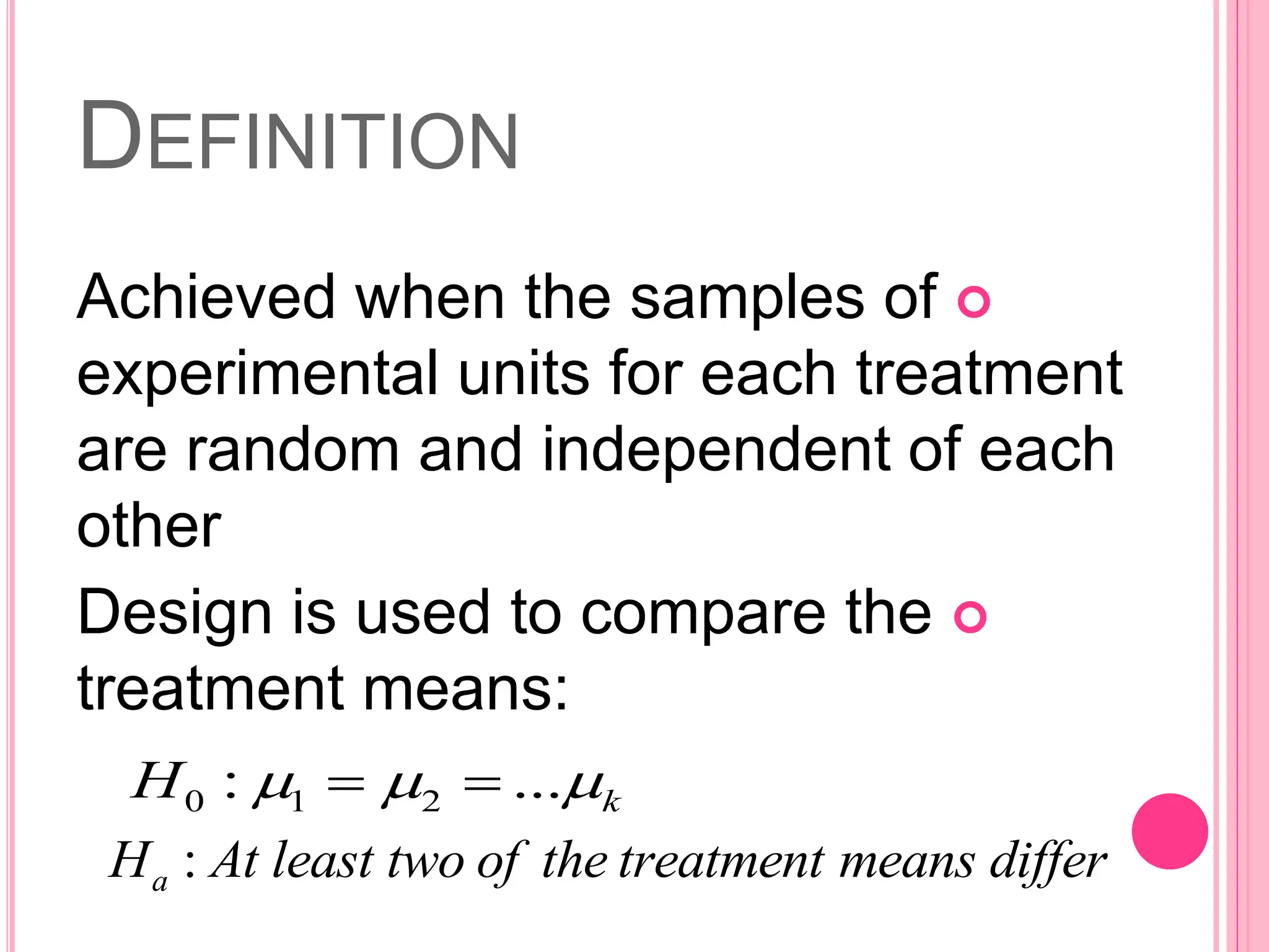
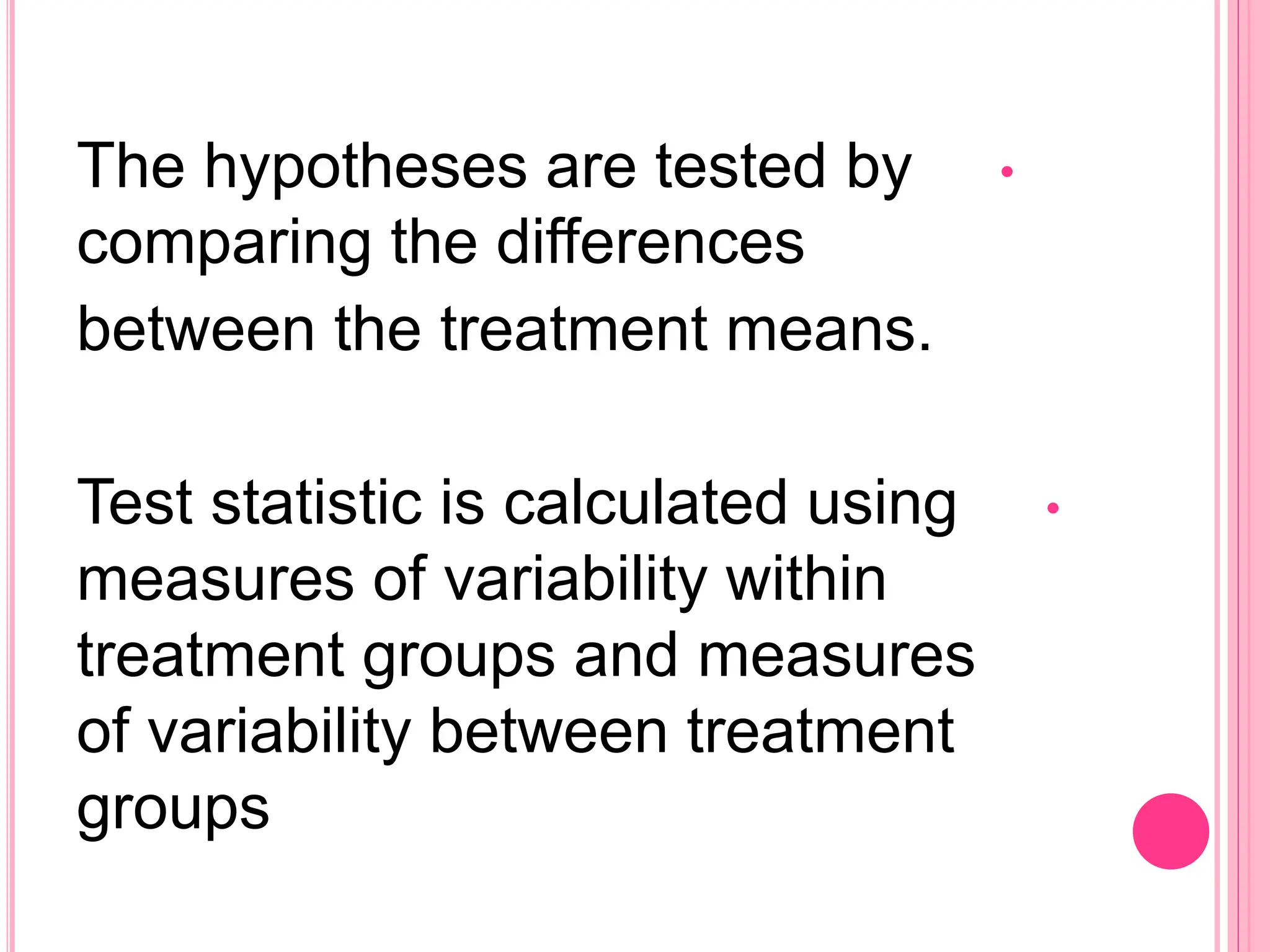
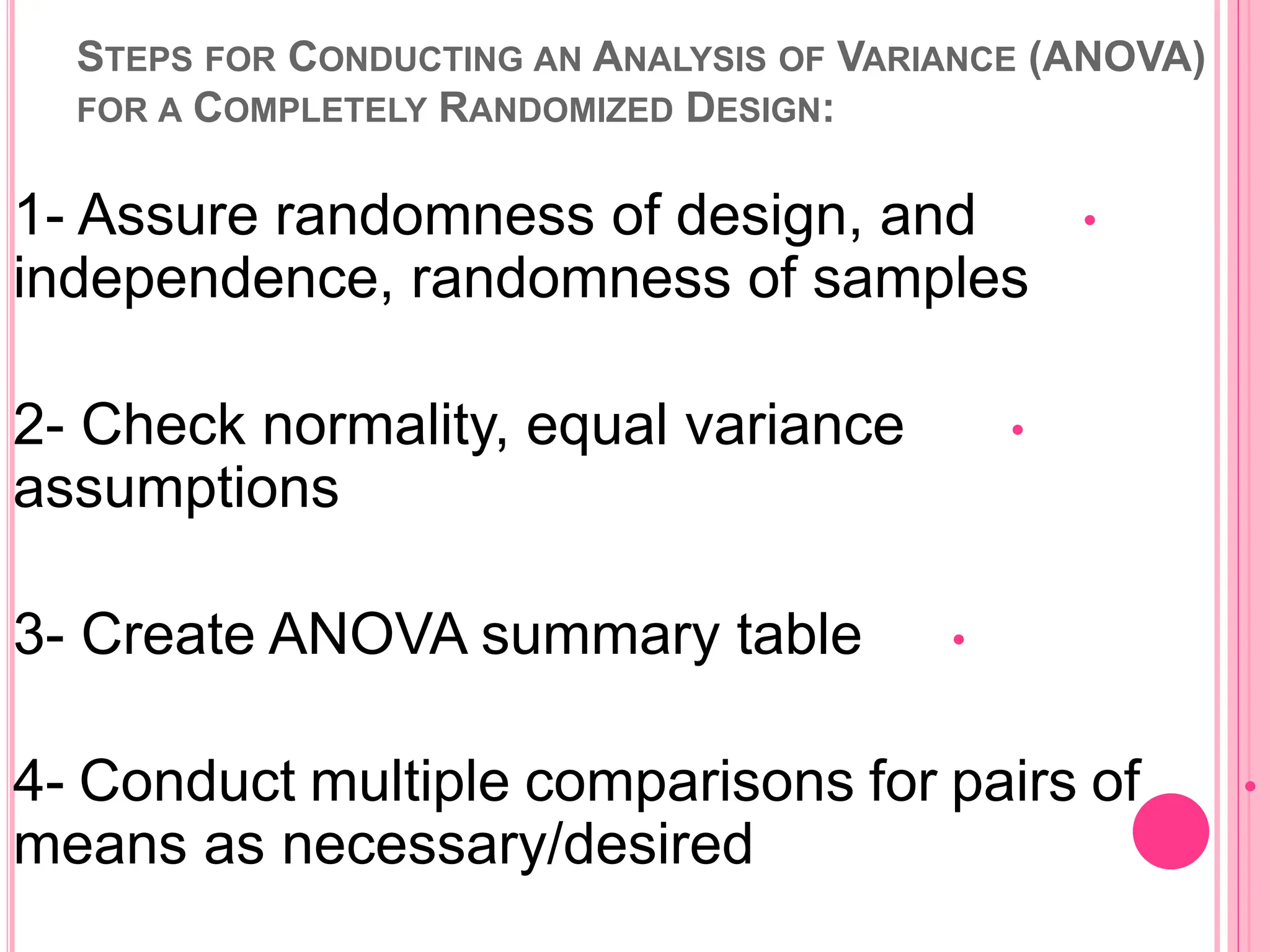
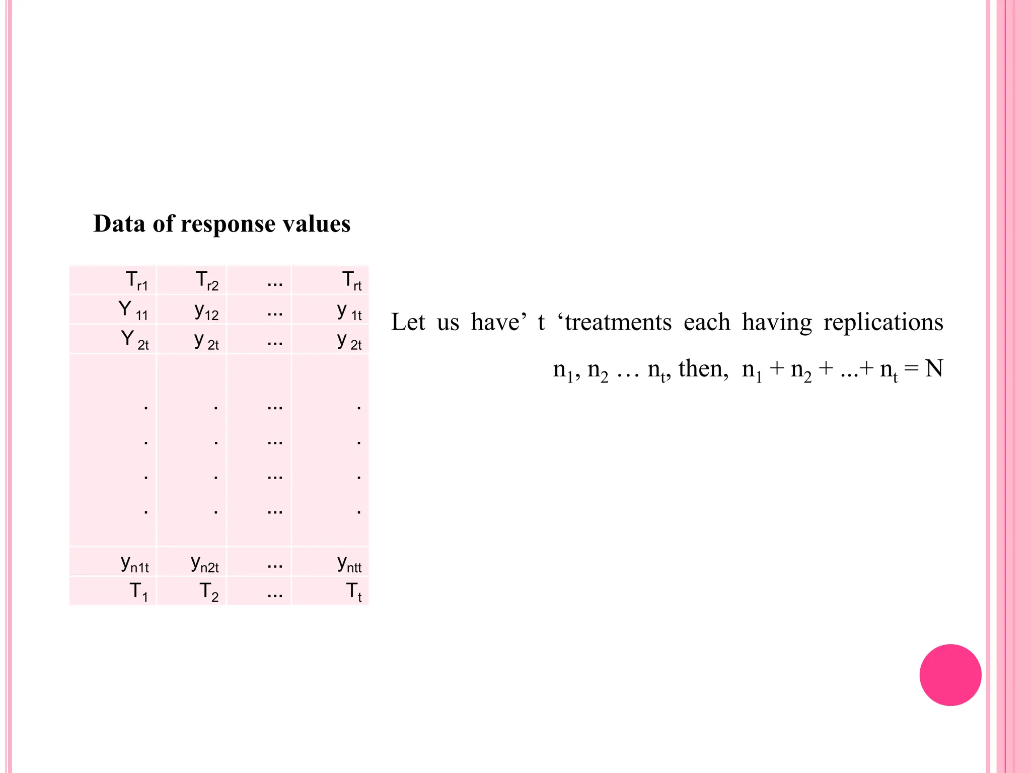
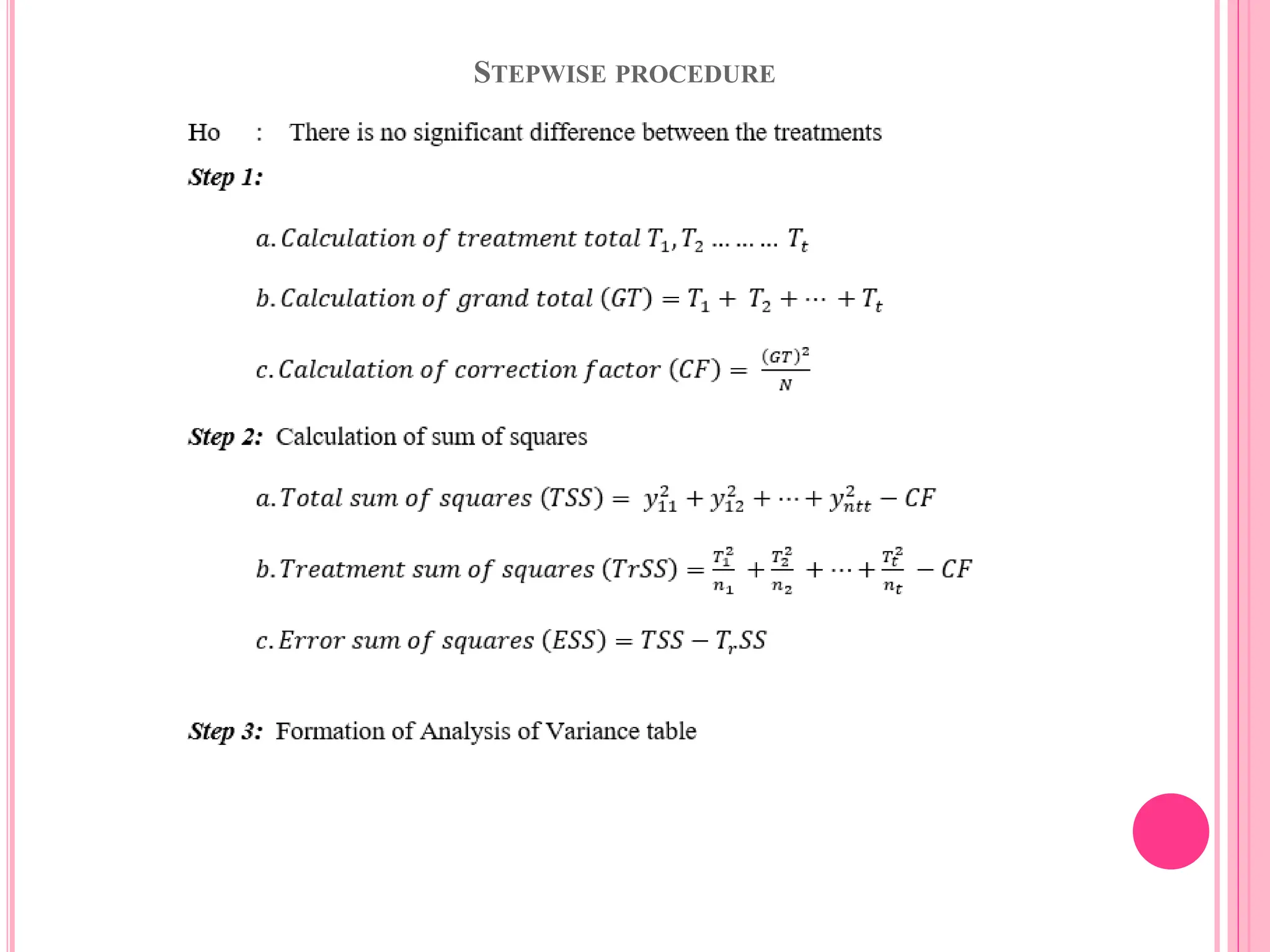
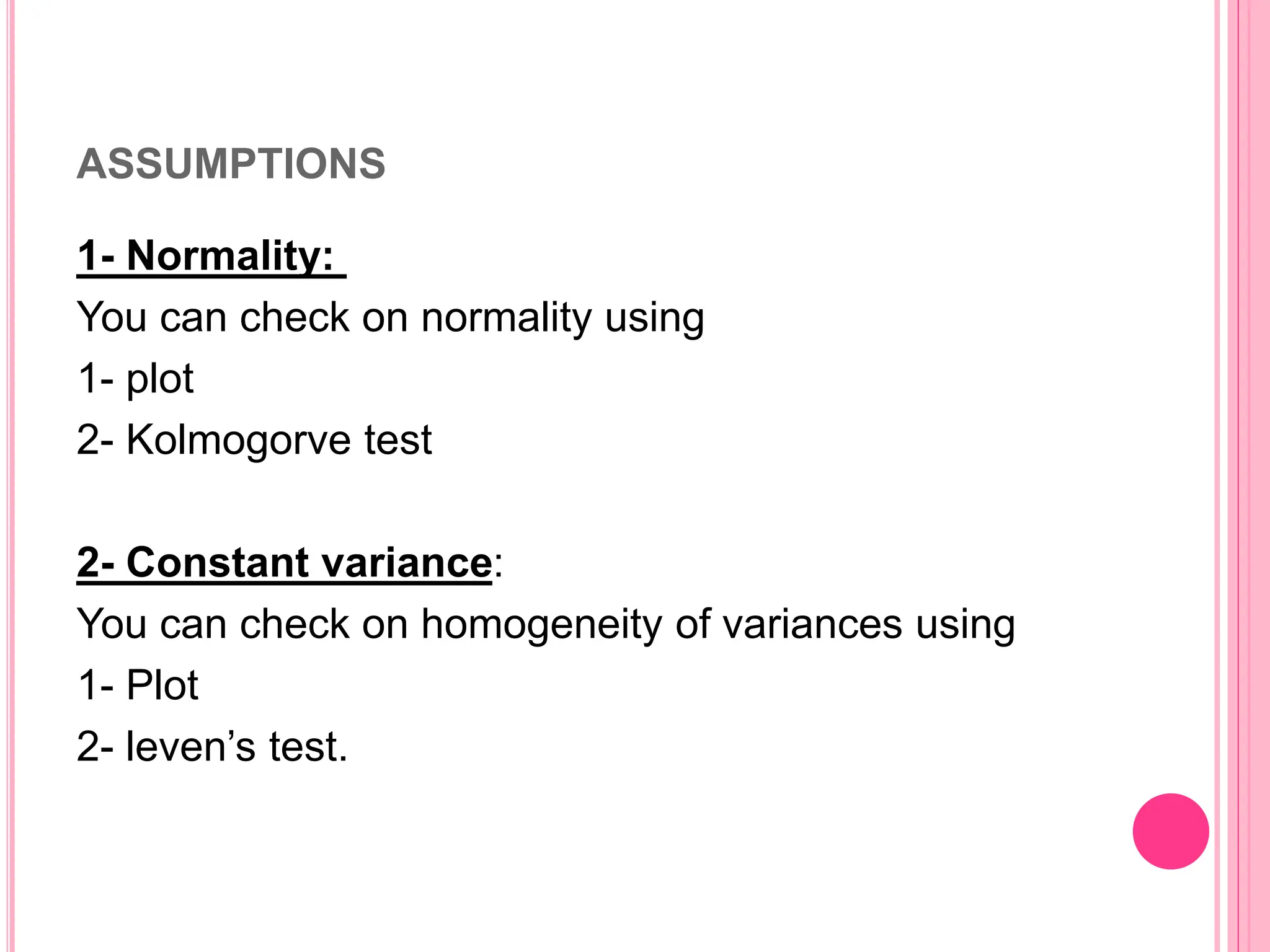
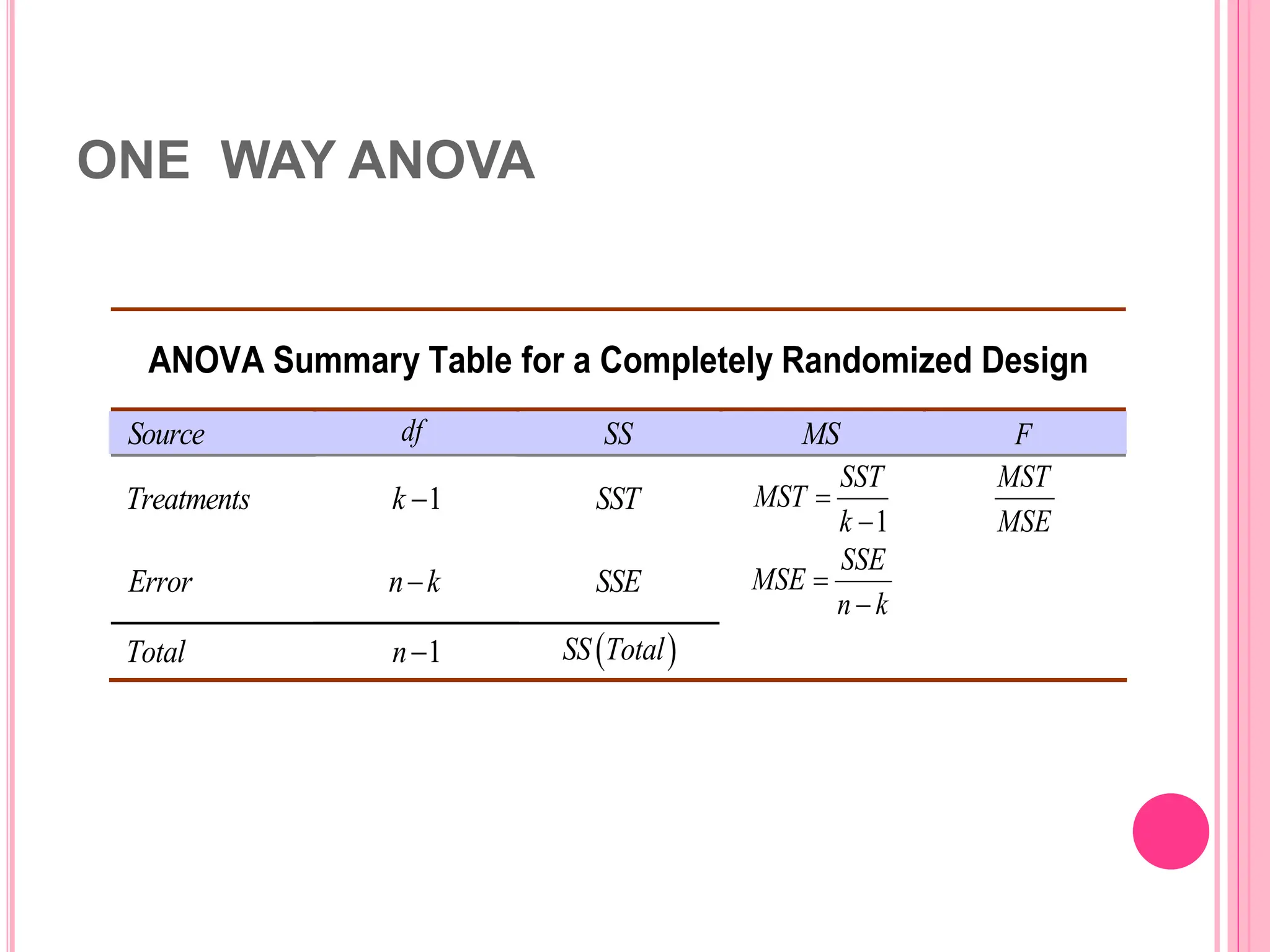
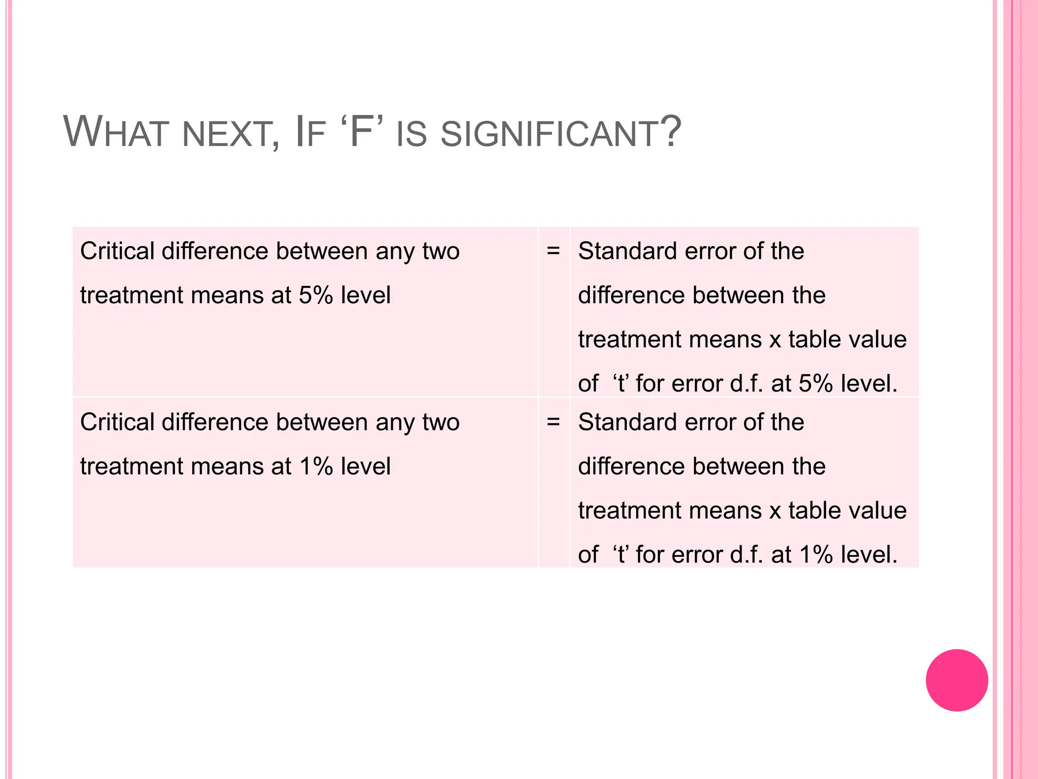
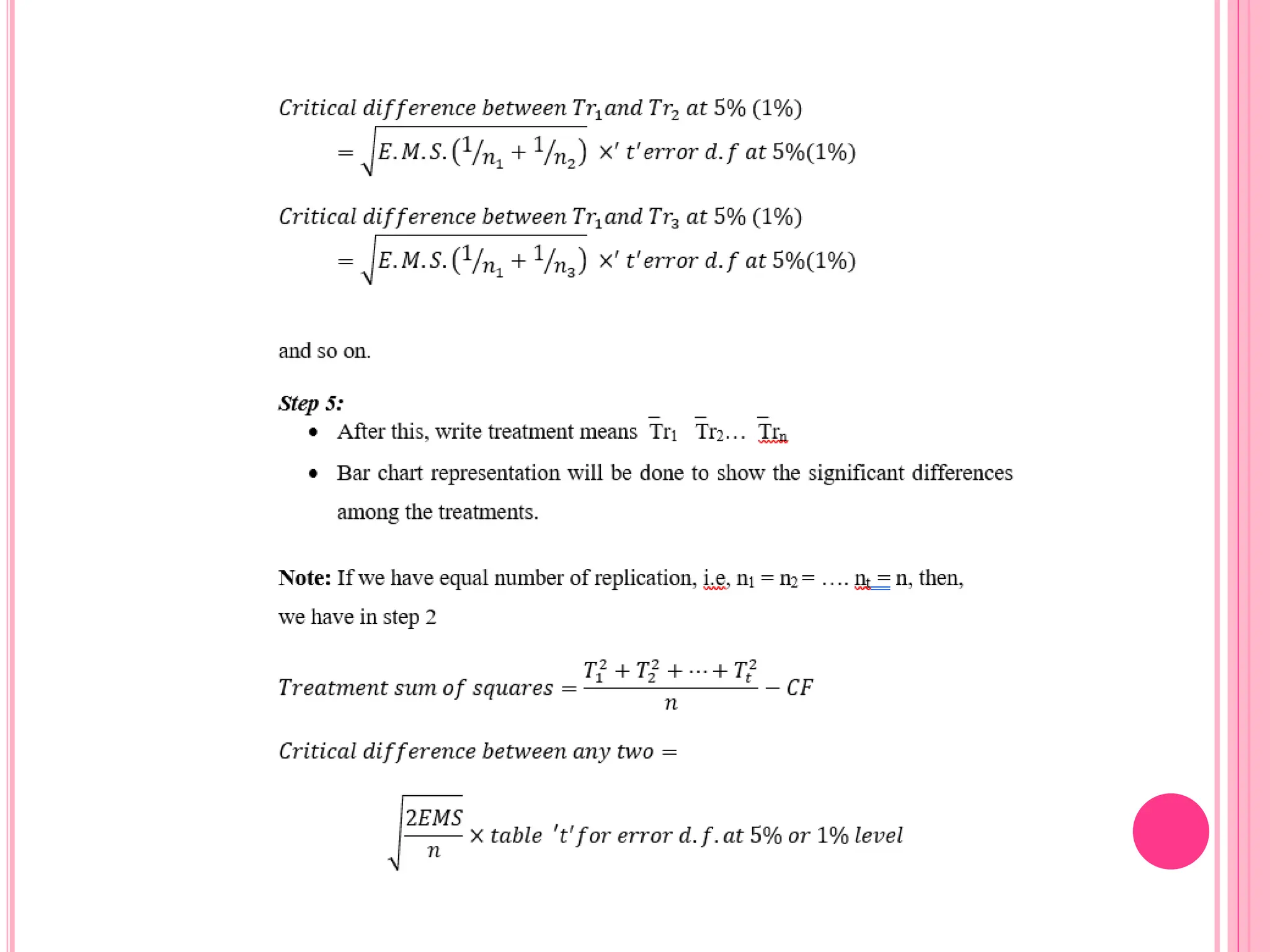
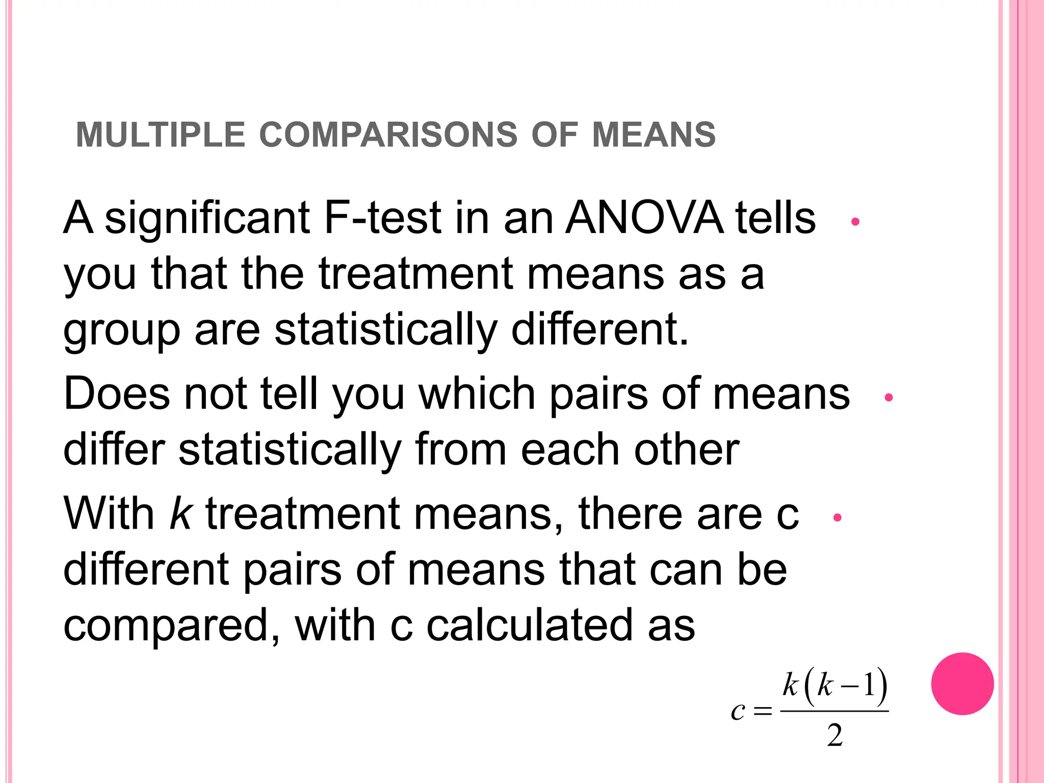
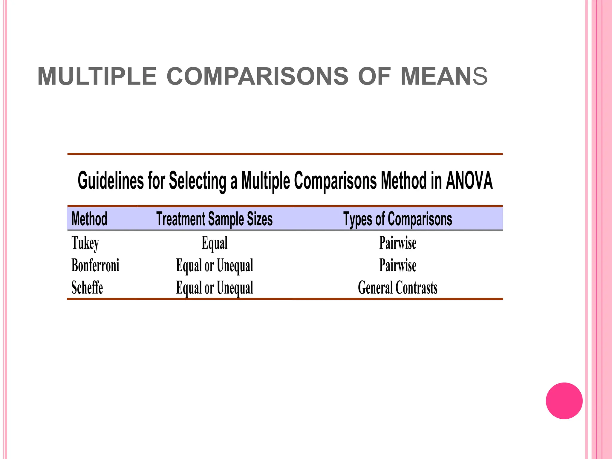
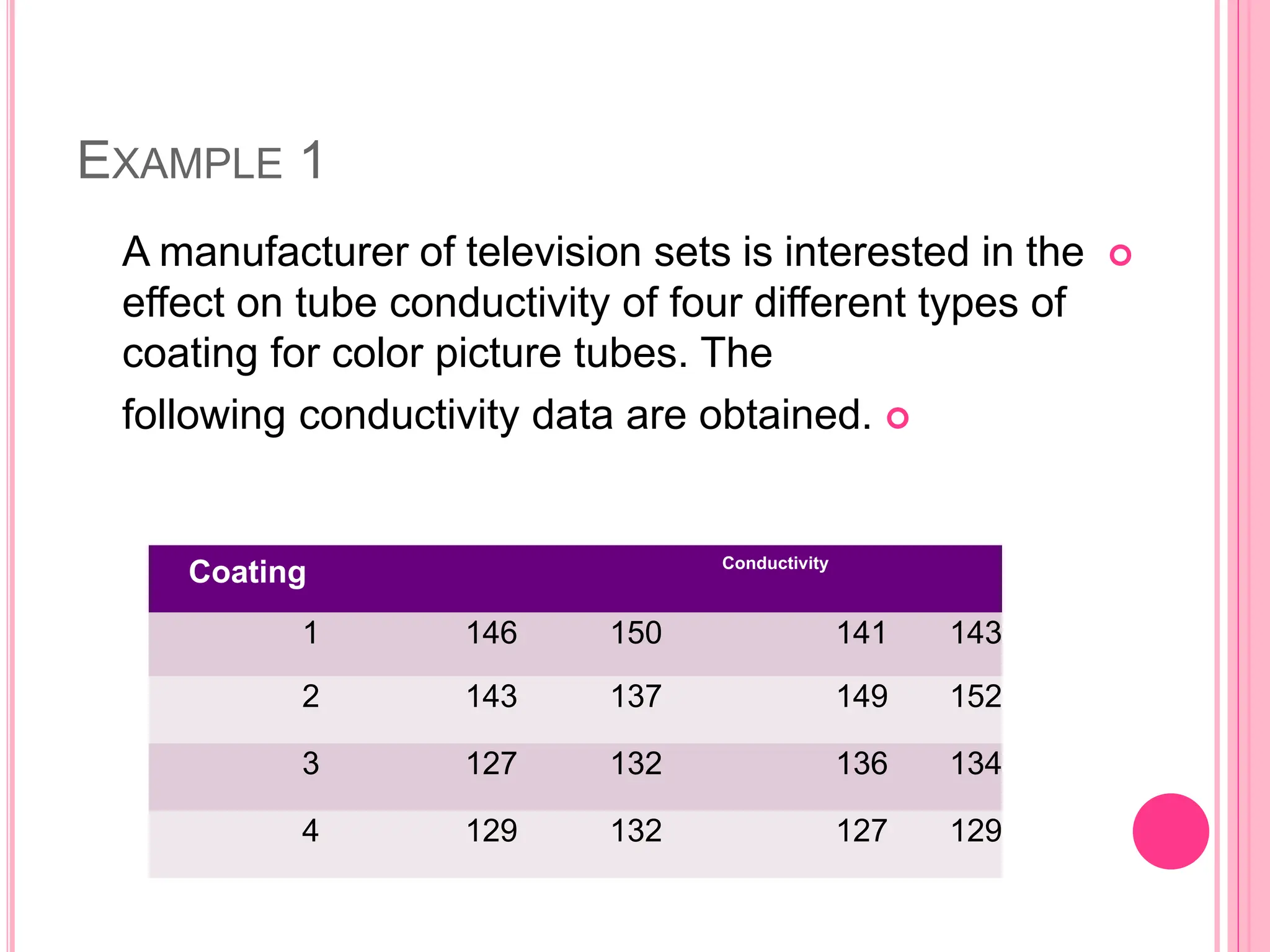
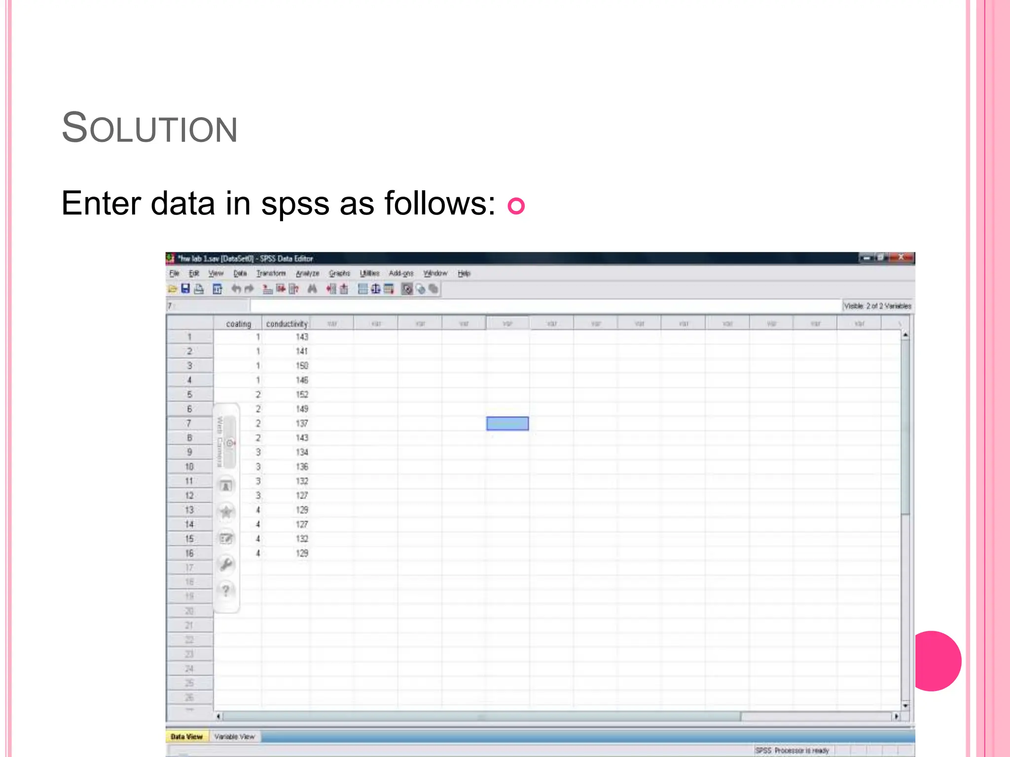
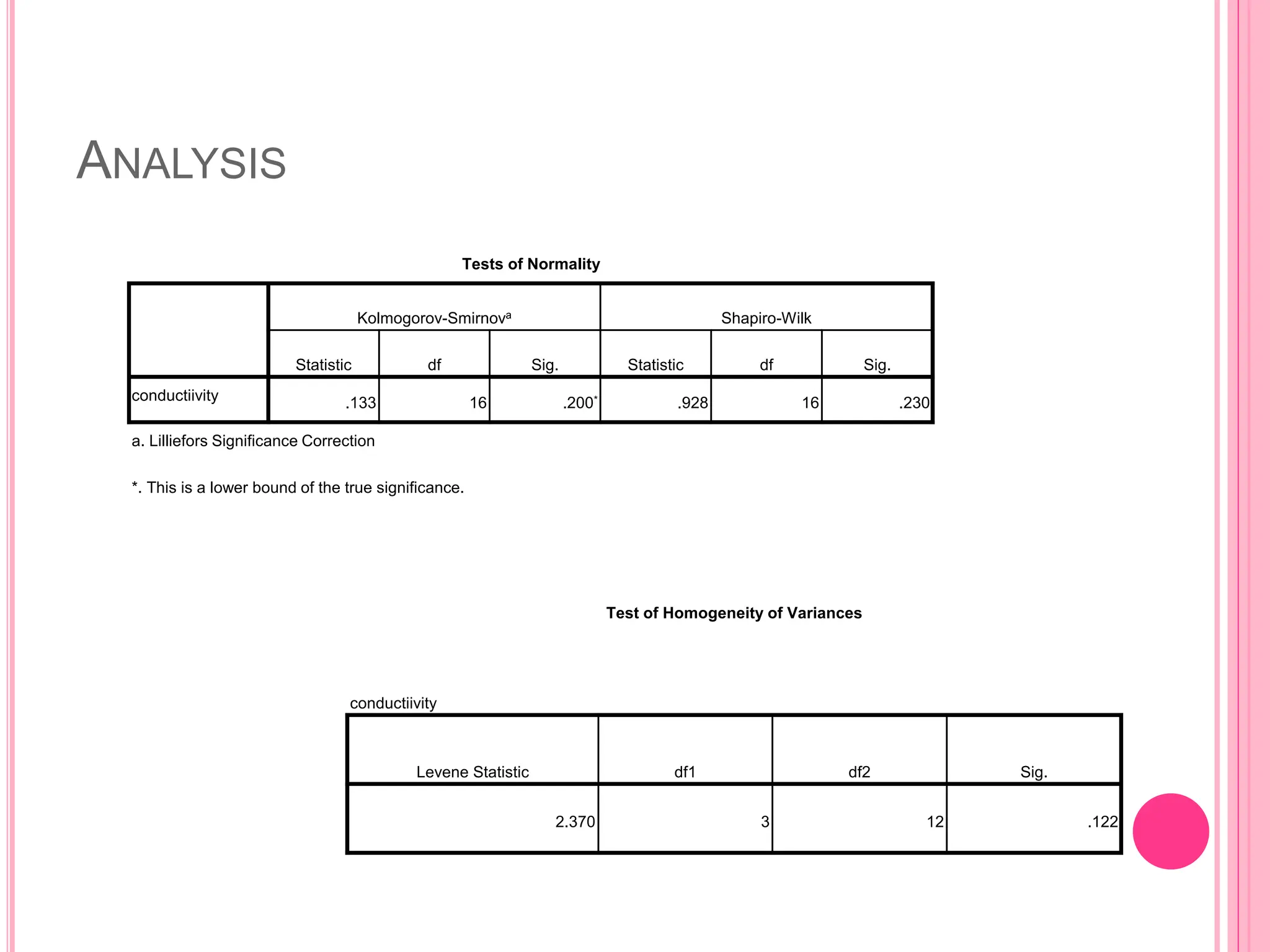
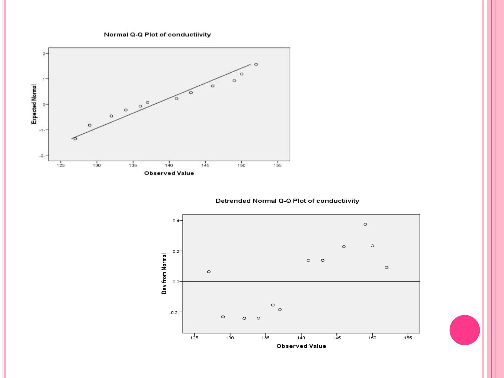
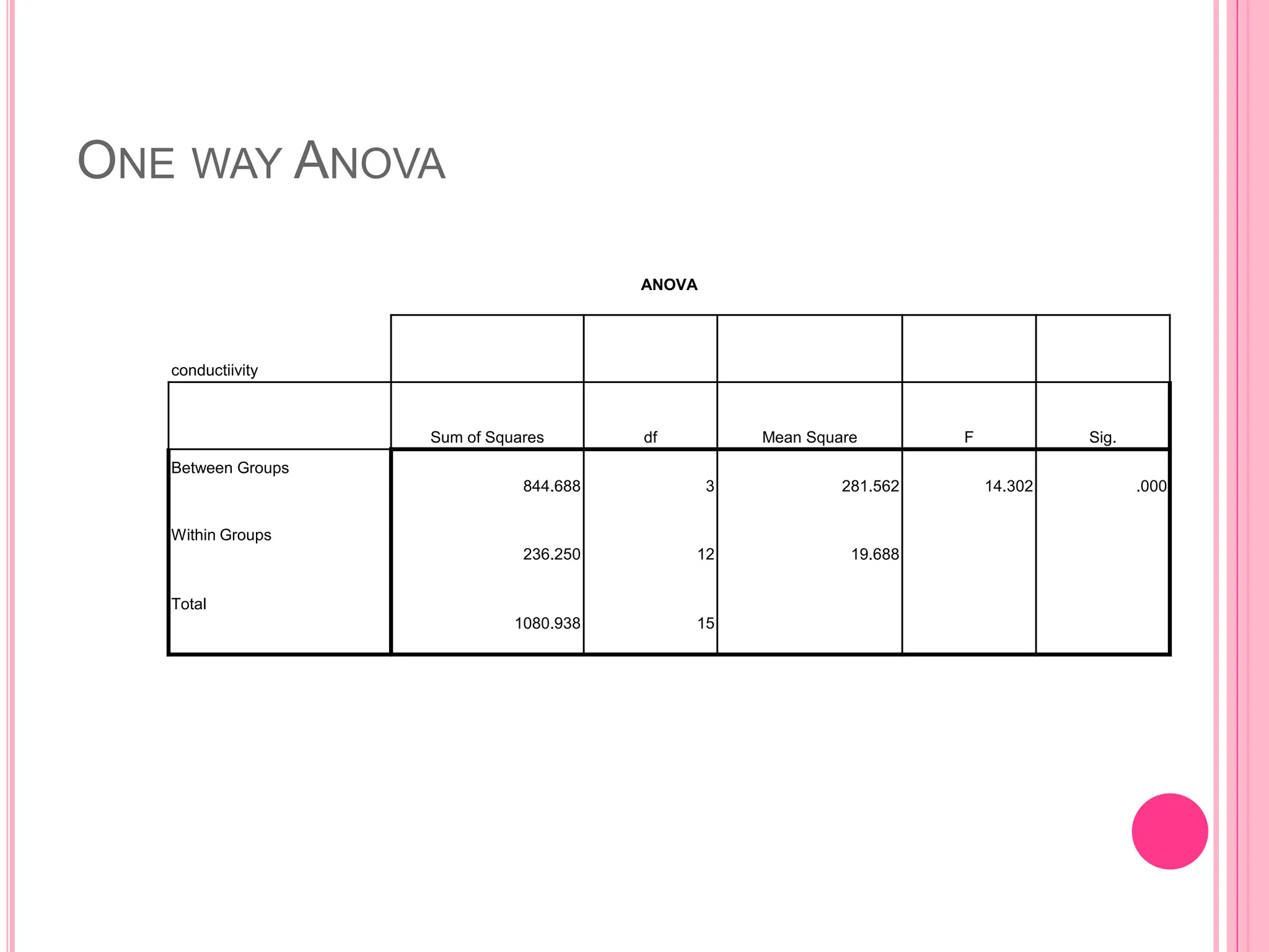
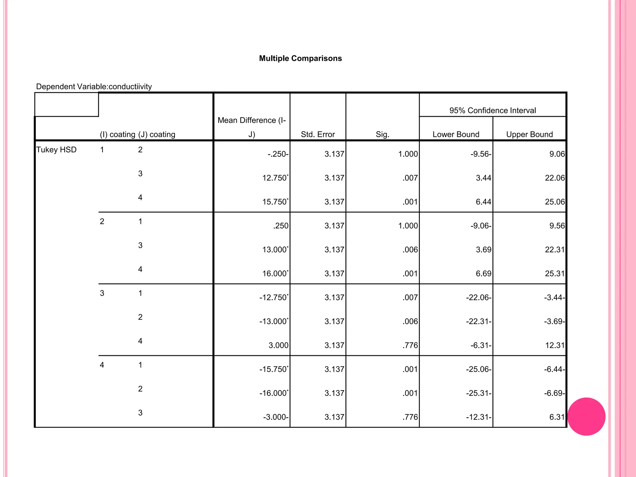
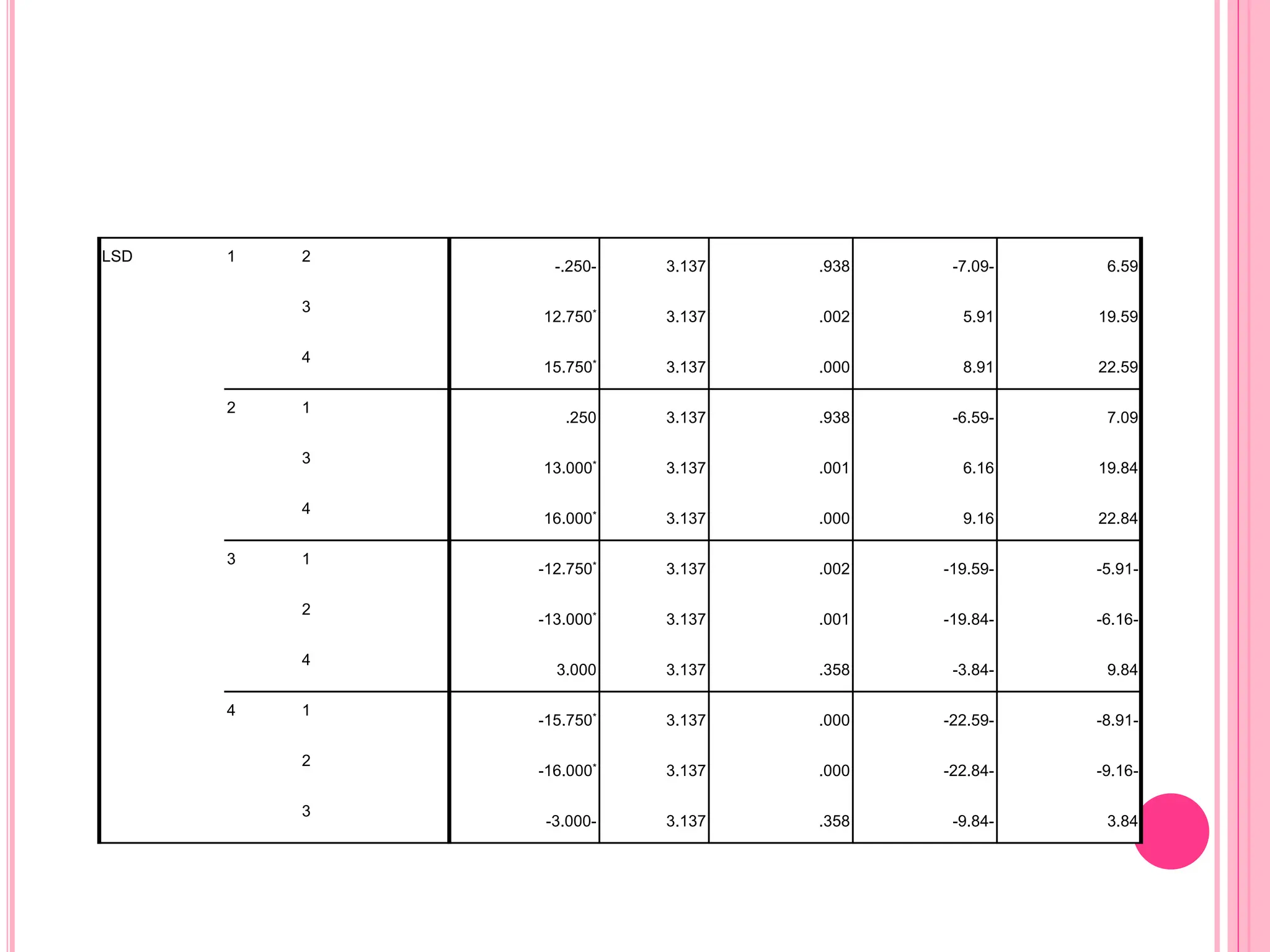
1. THE COMPLETELY
RANDOMIZED DESIGN
(CRD)
LAB # 1

2. DEFINITION

Achieved when the samples of
experimental units for each treatment
are random and independent of each
other

Design is used to compare the
treatment means:
0 1 2
: ... k
H   
 
:
a
H At least two of the treatment means differ

3. •
The hypotheses are tested by
comparing the differences
between the treatment means.
•
Test statistic is calculated using
measures of variability within
treatment groups and measures
of variability between treatment
groups

4. STEPS FOR CONDUCTING AN ANALYSIS OF VARIANCE (ANOVA)
FOR A COMPLETELY RANDOMIZED DESIGN:
•
1- Assure randomness of design, and
independence, randomness of samples
•
2- Check normality, equal variance
assumptions
•
3- Create ANOVA summary table
•
4- Conduct multiple comparisons for pairs of
means as necessary/desired

5. Tr1 Tr2 ... Trt
Y 11 y12 ... y 1t
Y 2t y 2t ... y 2t
.
.
.
.
.
.
.
.
...
...
...
...
.
.
.
.
yn1t yn2t ... yntt
T1 T2 ... Tt
Data of response values
Let us have’ t ‘treatments each having replications
n1, n2 … nt, then, n1 + n2 + ...+ nt = N

6. STEPWISE PROCEDURE

7. ASSUMPTIONS
1- Normality:
You can check on normality using
1- plot
2- Kolmogorve test
2- Constant variance:
You can check on homogeneity of variances using
1- Plot
2- leven’s test.

8. ONE WAY ANOVA
ANOVA Summary Table for a Completely Randomized Design
Source df SS MS F
Treatments 1
k  SST
1
SST
MST
k


MST
MSE
Error n k
 SSE
SSE
MSE
n k


Total 1
n  
SS Total

9. WHAT NEXT, IF ‘F’ IS SIGNIFICANT?
Critical difference between any two
treatment means at 5% level
= Standard error of the
difference between the
treatment means x table value
of ‘t’ for error d.f. at 5% level.
Critical difference between any two
treatment means at 1% level
= Standard error of the
difference between the
treatment means x table value
of ‘t’ for error d.f. at 1% level.

11. MULTIPLE COMPARISONS OF MEANS
•
A significant F-test in an ANOVA tells
you that the treatment means as a
group are statistically different.
•
Does not tell you which pairs of means
differ statistically from each other
•
With k treatment means, there are c
different pairs of means that can be
compared, with c calculated as
 
1
2
k k
c



12. MULTIPLE COMPARISONS OF MEANS
GuidelinesforSelectingaMultipleComparisonsMethodin ANOVA
Method TreatmentSampleSizes TypesofComparisons
Tukey Equal Pairwise
Bonferroni EqualorUnequal Pairwise
Scheffe EqualorUnequal GeneralContrasts

13. EXAMPLE 1

A manufacturer of television sets is interested in the
effect on tube conductivity of four different types of
coating for color picture tubes. The

following conductivity data are obtained.
Conductivity
Coating
143
141
150
146
1
152
149
137
143
2
134
136
132
127
3
129
127
132
129
4

14. SOLUTION

Enter data in spss as follows:

15. ANALYSIS
Test of Homogeneity of Variances
conductiivity
Levene Statistic df1 df2 Sig.
2.370 3 12 .122
Tests of Normality
Kolmogorov-Smirnova Shapiro-Wilk
Statistic df Sig. Statistic df Sig.
conductiivity .133 16 .200* .928 16 .230
a. Lilliefors Significance Correction
*. This is a lower bound of the true significance.

17. ONE WAY ANOVA
ANOVA
conductiivity
Sum of Squares df Mean Square F Sig.
Between Groups
844.688 3 281.562 14.302 .000
Within Groups
236.250 12 19.688
Total
1080.938 15

18. Multiple Comparisons
Dependent Variable:conductiivity
(I) coating (J) coating
Mean Difference (I-
J) Std. Error Sig.
95% Confidence Interval
Lower Bound Upper Bound
Tukey HSD 1 2
-.250- 3.137 1.000 -9.56- 9.06
3
12.750* 3.137 .007 3.44 22.06
4
15.750* 3.137 .001 6.44 25.06
2 1
.250 3.137 1.000 -9.06- 9.56
3
13.000* 3.137 .006 3.69 22.31
4
16.000* 3.137 .001 6.69 25.31
3 1
-12.750* 3.137 .007 -22.06- -3.44-
2
-13.000* 3.137 .006 -22.31- -3.69-
4
3.000 3.137 .776 -6.31- 12.31
4 1
-15.750* 3.137 .001 -25.06- -6.44-
2
-16.000* 3.137 .001 -25.31- -6.69-
3
-3.000- 3.137 .776 -12.31- 6.31

19. LSD 1 2
-.250- 3.137 .938 -7.09- 6.59
3
12.750* 3.137 .002 5.91 19.59
4
15.750* 3.137 .000 8.91 22.59
2 1
.250 3.137 .938 -6.59- 7.09
3
13.000* 3.137 .001 6.16 19.84
4
16.000* 3.137 .000 9.16 22.84
3 1
-12.750* 3.137 .002 -19.59- -5.91-
2
-13.000* 3.137 .001 -19.84- -6.16-
4
3.000 3.137 .358 -3.84- 9.84
4 1
-15.750* 3.137 .000 -22.59- -8.91-
2
-16.000* 3.137 .000 -22.84- -9.16-
3
-3.000- 3.137 .358 -9.84- 3.84

20. Thanks for all