SlideShare a Scribd company logo
StreamTemp Model – Page 1
Boise River StreamTemp Model
1 Introduction
City of Boise personnel have developed stream temperature model scenarios of the Boise River
to describe existing instream temperature characteristics, and identify best attainable conditions.
These scenarios used the model SNTEMP (Bartholow 2010). The SNTEMP model results have
been presented in previous permit reapplications to identify effluent effects on the temperature
regime in Boise River. SNTEMP has now been updated to StreamTemp for Windows by
Thomas R. Payne & Associates, who have adapted the original code to be accessible by a
Windows interface. StreamTemp is being applied to the current permit reapplication process as
it relates to stream temperature.
1.1 StreamTempModel
StreamTemp is a mechanistic model that predicts the minimum, mean, and maximum daily water
temperatures. Mechanistic refers to simulation of heat flux processes that contribute to stream
temperature, including incoming solar radiation and reflected longwave radiation, atmospheric
radiation, vegetative and topographic shading, evaporation, convection, conduction, and friction,
which is governed by the stream gradient and roughness. Figure 1 shows the mean daily heat
flux components calculated for one model reach.
Figure 1. Example annual mean daily heat flux components.
Darcy Sharp,Environmental Data Analyst
Environmental Division,PublicWorks Department
City of Boise; 11/8/2016
StreamTemp Model – Page 2
Positive heat flux components are a heat gain to the system and negative components are heat
loss from the system. These components illustrate the driving forces in heating and cooling.
1.2 TemperatureCriteria
The 2016 StreamTemp model predicts the Boise River thermal response under alternative
scenarios to help identify and interpret:
 The proportion of the thermal load that is due to effluent flows and temperatures
 Potential thermal load offset quantification
Lander Water Renewal Facility (WRF) and West Boise WRF discharge to assessment unit (AU)
ID17050114SW005_06, the reach from Veterans Memorial Parkway to Star Bridge. This AU is
listed as impaired for temperature (DEQ 2014)
These AUs are designated for the beneficial uses of Cold Water Aquatic Life (CWAL),
Salmonid Spawning (SS) and Primary Contact Recreation. Temperature criteria that apply to
these AUs include:
 The CWAL criteria in IDAPA 58.01.02.250.02.b: “Water temperatures of twenty-two
(22) degrees C or less with a maximum daily average of no greater than nineteen (19)
degrees C.”
 The site-specific SS criteria in IDAPA 58.01.02.278: “A maximum weekly maximum
temperature of thirteen degrees C (13°C) to protect brown trout, mountain whitefish, and
rainbow trout spawning and incubation applies from November 1 through May 30.”
 IDAPA 58.01.02.010.59. Maximum Weekly Maximum Temperature (MWMT). “The
weekly maximum temperature (WMT) is the mean of daily maximum temperatures
measured over a consecutive seven (7) day period ending on the day of calculation.
When used seasonally, e.g. spawning periods, the first applicable WMT occurs on the
seventh day into the time period. The MWMT is the single highest WMT that occurs
during a given year or other period of interest, e.g., a spawning period.”
According to a memo referenced in Appendix E of the draft Third Edition of the Idaho
Department of Environmental Quality Water Body Assessment Guidance (DEQ 2016), the
following procedures apply to determination of temperature impairment:
 The time period of interest to gage frequency of exceedance for CWAL temperature
criteria is the 93-day period of June 21st through September 21st
 If the frequency of exceedance is less than 10%, DEQ has the discretion to determine
there is no impairment for temperature
2 Methods
This section describes the steps used in setting up, calibrating, and running the StreamTemp
model for the Boise River. Model extent and data sources are described.
StreamTemp Model – Page 3
2.1 ModelSetup and Data Sources
The model is initialized by entering the time records and dates for each model run. Annual daily
records (January 1 to December 31) are selected for the Boise River model. Having an annual
output of daily predictions allows interpretation of results on a seasonal, monthly, or weekly
basis as needed. Regulatory issues may require evaluation of winter as well as summer limits.
2.1.1 Network Design
The spatial extent of the StreamTemp model is from Lucky Peak to Middleton (Figure 2). The
study reach includes the following AUs listed for temperature:
 ID17050114SW005_06, extending from Veteran’s to Star
 ID17050114SW005_06a, extending from Star to Middleton
Figure 2. Spatial extent of StreamTempmodel of Boise River.
The network design data entry includes a node title, location, and elevation at the top and bottom
of each reach. StreamTemp automatically calculates the distance between nodes and the azimuth
of the reaches. Table 1 provides the data entered in the network design screen.
Table 1. Network design parameters for Boise River StreamTempmodel.
Node Title Elevation (ft) Latitude Longitude
Lucky Peak 2815 43.5378 -116.0934
Diversion Dam 2756 43.5652 -116.1319
Suez Water 2726 43.5833 -116.1606
Marden Footbridge 2684 43.6055 -116.2035
Veteran’s Bridge 2654 43.6364 -116.2430
Lander WRF 2611 43.6386 -116.2443
Glenwood Bridge 2595 43.6673 -116.2994
Loss to North Channel 2581 43.6719 -116.3265
West Boise WRF 2569 43.6729 -116.3317
Eagle Bridge South Channel 2520 43.6740 -116.4080
Gain from N Channel and Star 2472 43.6813 -116.4898
Middleton Gage 2411 43.6870 -116.5868
End 2405 43.6780 -116.5944
StreamTemp Model – Page 4
A proportional schematic of the network design is shown in Figure 3. The view has been rotated
30° to ensure legibility of the labels.
Figure 3. Schematic of the model reaches for Boise River StreamTempmodel.
The south channel is simulated in the model network, but the north channel is not. Instead, the
north channel is accounted for by streamflow loss and gain in the appropriate model reaches.
2.1.2 Reach Physical Geometry
The reach physical geometry input screen includes azimuth, latitude, friction coefficients, width
constant and coefficient, and thermal gradient coefficient. Typically, geometry analyses will
include rating curves developed from channel measurements. Rating curves generally follow the
format:
𝑈 = a𝑄 𝑏
and 𝐻 𝑜𝑟 𝑊 = α𝑄 𝛽
,
StreamTemp Model – Page 5
where U and H are velocity and height (or width) and where a, b, α, and β are empirical
coefficients that are determined from velocity-discharge and stage-discharge rating curves,
respectively. However, there are not enough existing channel data to develop rating curves for
this temperature analysis.
StreamTemp uses width constants and coefficients to describe channel geometry. Without
channel measurements to develop rating curves, the width constant can be used to describe the
width of the channel and the coefficient can be left at zero. The disadvantage of this method is
that the physical geometry must be re-calibrated for each hydrologic scenario. The following
figures show the difference between using a width coefficient and setting this coefficient to zero.
Figure 4. Channel geometry of Veteran’s Bridge reach with V-shaped channel described by width constant
and coefficient.
Figure 5. Channel geometry of Veteran’s Bridge reachwith square channel described by width constant
alone.
StreamTemp is not a hydrology model, but it accounts for a water balance in each model reach.
The size and shape of the channel affects the depth of the given streamflow. The same volume
StreamTemp Model – Page 6
of water in a flat, broad channel will be warmer than in a narrow, V-shaped channel since more
surface area is exposed to incoming solar radiation. The higher water column has a buffering
effect on temperature extremes.
This effect was apparent during temperature calibration of the Boise River scenarios. Simulating
a V-shaped channel geometry smoothed the daily temperature predictions in the winter, but the
actual monitoring data was showing large daily fluctuations. By applying the square-sided
channels throughout the model reaches, temperature predictions became more accurate and were
able to match the daily fluctuations in the winter. Table 2 provides the reach geometry
parameters used for the calibrated existing conditions model.
Table 2. Reach geometry worksheet from calibrated model.
Reach Name Azimuth
(degrees)
Friction Coefficient
(unitless)
Width Constant
(feet)
Width
Coefficient
Thermal
Gradient
Lucky Peak 313.71 0.0430 100 0 1.65
Diversion Dam 310.35 0.0430 150 0 1.65
Suez Water 304.9 0.0350 59 0 1.65
Marden 316.63 0.0350 186 0 1.65
Veterans 335.16 0.0350 390 0 1.65
Lander WRF 310.69 0.0430 275 0 1.65
Glenwood Bridge 282.65 0.0300 62 0 1.65
Loss to North Channel 284.54 0.0350 83 0 1.65
West Boise WRF 270.70 0.0350 104 0 1.65
EagleSouth Channel 306.85 0.0350 117 0 1.65
Gain from North Channel 274.34 0.0350 139 0 1.65
Middleton Gage 269.52 0.0350 169 0 1.65
2.1.3 Hydrology Data
The USGS 13202000 “Boise River nr Boise ID” streamgage is just downstream of Lucky Peak
and represents the headwaters of the study reach. This streamgage has an extensive period of
record of discharge measurements from 1895 through 2016. However, a water management
agreement was reached in the Boise River valley starting on March 12, 1982 (U.S. Bureau of
Reclamation 1984). The discharge measurements from this date through 2016 will be used to
represent current hydrological conditions. The flow duration curve for current water
management is shown in Figure 6.
The 95th percentile low flow is 150 cubic feet per second (cfs), which means that 95% of the
daily average streamflow records have been higher than 150 cfs. The 75th percentile flow is 250
cfs. This has typically been the streamflow from November through March, as shown in the
discharge record in Figure 7.
StreamTemp Model – Page 7
Figure 6. Flow duration curve for USGS 13202000 from March 1, 1982 through 2016 for current water
management.
Figure 7. Daily average streamflow at USGS 13202000 from March 1, 1982 through 2016.
The streamgage USGS 13206000 “Boise River at Glenwood Bridge nr Boise ID” is between
Lander and West Boise. The flow duration curve is provided in Figure 8.
StreamTemp Model – Page 8
Figure 8. Flow duration curve at Glenwood from March 1, 1982 through August 22, 2016.
The USGS 13206305 Boise River South Channel at Eagle ID is downstream of West Boise. The
flow duration curve for this location is provided in Figure 9. The Glenwood and Eagle
streamflow records were used to correct the water balance in the middle and near the end of the
temperature study reach.
Figure 9. Flow duration curve at Eagle from November 1, 1999 through August 22, 2016.
StreamTemp Model – Page 9
Note that this streamgage has a shorter record of operation, beginning in 1999.
2.1.3.1 Selection of Representative Flow Years
The temperature study is based on an extreme low flow scenario which represents the most
critical conditions, and a median flow year which represents typical current conditions.
The 95th percentile low flow 150 cfs occurred most frequently in 1983, but Boise City stream
temperature monitoring dates back to 2000. In this timeframe, low flows of 152 and 153 cfs
occurred during calendar years 2001 and 2002. Examining 2001 and 2002 weather data from the
Boise AgriMet station for the warmest conditions shows that 2001 had 84 days where the
maximum temperature was greater than 86°F, which is the temperature that stresses plant
growth. In comparison, 2002 only had 34 days >86°F. See Table 3 for a brief data summary of
air temperatures in 2001 and 2002.
Table 3. Summary of air temperatures at Boise AgriMet weather station for 2001 and 2002.
Air Temperature Parameter 2001 2002
Maximum daily mean (°F) 85 89
Maximum daily maximum(°F) 102 99
Days maximum temperature >86(°F) 84 34
The weather in 2001 presented more heat stress factors, so that is the year selected to represent
the 95th percentile low flow scenarios. The annual flow record for this year is used to represent
the headwaters of this scenario.
To represent more typical hydrology, 2014 is chosen as a median flow year. The 75th percentile
flow released from Lucky Peak Dam is 250 cfs. This has typically been the streamflow from
November through March under the 1982 water management agreement.
2.1.3.2 Hydrology Data Entry
The StreamTemp hydrology data screen provides options for each reach to include diversion,
point or return flows. Streamflow data from USGS 13202000 and temperature data from Boise
City are entered at the top reach. The Idaho Department of Water Resources (IDWR) accounts
for diversion and return flows. Water rights accounting data is found at
https://maps.idwr.idaho.gov/qWRAccounting/. Table 4 documents the location and data sources
for hydrology and stream temperature, with river mile defined from Boise River confluence with
Snake River to the upstream location.
Table 4. Data sources and location for StreamTemphydrology.
River Streamflow US Geological Survey (USGS) and
Idaho Department of Water Resources (IDWR) Stations
River Mile
USGS 13202000 Boise River nr BoiseID 63.6
USGS 13206000 Boise River at Glenwood Bridge nr Boise ID 47.7
USGS 13206305 Boise River SouthChannel at Eagle ID 42.8
USGS andIDWR 13210050 Boise River nr Middleton ID 31.4
Diversion Hydrology IDWR station with discharge data
13202011 DiscoveryPark 63.3
13202995 PenitentiaryCanal 61.2
13203000 New York Canal below DiversionDam 61.2
13203600 Boise River below DiversionDam 61.1
StreamTemp Model – Page 10
13203527 Surprise Valley/Micron 60.6
13203715 Shakespeare Festival 58.8
13203760 Ridenbaugh Canal 58.3
13203781 Williams Park 58.0
13204005 Bubb Canal 57.5
13204015 Herrick 57.1
13204020 Meeves Canal 56.8
13204060 Rossi Mill Canal 56.4
13204200 UnitedWater (Now Suez) 56.1
13204190 Boise CityCanal 55.9
13205514 Kathryn Albertson 52
13205515 Settlers Canal 52
13205517 FairviewAcres 51.8
13205613 Boise CityParks 51.5
13205622 Thurman Mill Canal 51.1
13205617 Drainage District #3 51
13205640 Farmers UnionCanal 50.4
13205642 Boise River at Veteran’s MemorialPark 50.2
13205984 Riverside Village 47.8
13206000 Boise River at Glenwood Bridge 47.7
13206090 New DryCreek Canal 45.6
13206096 Woods 45
13206205 Lemp Canal 44.8
13206220 Warm Springs Canal 44.5
13206270 Conway-Hamming Canal 43.5
13206290 Thomas AikenCanal 43.1
13206292 Mace-CatlinCanal 43.1
13206260 Graham-Gilbert Canal 42.9
13208738 Barber Pumps 42.4
13208740 Seven Suckers Canal 42
13209450 Thurman Drain 41.9
13209480 Phyllis Canal 41.4
13209990 Canyon CountyCanal 36.3
13210005 Caldwell Highline Canal 36.3
13210012 Otter Mitigation 35.7
River Temperature City of Boise
BR07 LuckyPeak 63.6
BR06 Marden Footbridge 54.8
BR05 Veteran’s Memorial ParkBridge 50.2
BR04 GlenwoodBridge 47.7
BR03 Eagle Bridge southchannel 42.8
BR02 Middleton 31.4
Facility Volume and
Temperature
City of Boise
Lander Water RenewalFacility 50
West Boise Water RenewalFacility 44.2
Locations for the 39 diversions and monitoring sites are shown in Figure 10.
StreamTemp Model – Page 11
Figure 10. StreamTempmodel extent and data sources.
The key input features in each of the model reaches are shown in Table 5. This table shows
where the diversions are withdrawn from each model reach.
Table 5. StreamTempmodel reachdescriptions.
Model
Reach
River Mile Reach Name Data Source Name and USGS or IDWR Site Number
City of Boise Stream and Effluent Temperature
1 63.6 to 61.2 LuckyPeak LuckyPeak, DiscoveryPark, PenitentiaryCanal
2 61.1 to 58.3 DiversionDam New York Canal, Surprise Valley/Micron, Shakespeare Festival, Ridenbaugh
3 58.2 to 56.1 Suez Water Williams Park, Bubb, Herrick, Meeves, Rossi, Suez
4 56.0 to 53.1 Marden
Footbridge
Boise CityCanalwithdrawal andMarden sampling location
5 53.0 to 50.1 Veteran’s
Bridge
Settler’s, Kathryn Albertson, Fairview Acres, Boise City Parks, ThurmanMill,
Farmer’s Union, Veteran’s sampling location
6 50.0 to 47.9 Lander WRF Lander input
7 47.8 to 45.6 Glenwood
Bridge
Riverside Village, Glenwood samplinglocation, NewDryCreek Canal
8 45.5 to 44.5 Loss to North
Channel
Loss to North Channel, Woods. LempCanal, Warm Springs Canal
9 44.4 to 43.6 West Boise
WRF
West Boise input
StreamTemp Model – Page 12
10 43.5 to 40.1 Eagle Bridge
South Channel
Conway-Hamming, Thomas Aiken, Mace-Catlin, Graham-Gilbert, Barber Pumps,
Seven Suckers andPhyllis Canal withdrawals;ThurmanDraininputs;Eagle
Bridge sampling location
11 40.2 to 36.4 Gainfrom
North Channel
Gainfrom NorthChannel to 1321000--Boise River near Star
12 36.3 to 31.1 Middleton
Gage
Canyon CountyCanal, Caldwell Highline Canal, Otter withdrawal; 13210050
Boise River near Middleton
13 31.0 End
2.1.4 Weather Data
StreamTemp requires average air temperature, humidity, percent sunshine, wind speed and solar
radiation to simulate stream temperatures. The weather data entry screen also requires the
latitude and station elevation to calculate adiabatic lapse rate changes for stream reach
elevations. There are also options for setting global constants and coefficients to describe local
climate.
The Boise AgriMet weather station at http://www.usbr.gov/pn/agrimet/webarcread.html provided
the meteorology data for the Boise River temperature model. Although StreamTemp can
calculate low and high air temperatures from average data, the Boise AgriMet station provided
minimum and maximum daily air temperatures along with daily average. Having real data for
the minimum and maximum air temperatures improved the calibration. The global constants and
coefficients were left at default.
2.1.5 Shade Data
For shade input parameters, the user can input percent shade if that value is known, or
StreamTemp will calculate percent shade from reach azimuth, total stream corridor width,
vegetation offset, and topographic shade. Temperature predictions improved slightly when
StreamTemp was allowed to automatically fill percent shade values that varied daily for each
model reach. Final parameters used by the model to calculate shade are shown in Table 6.
Table 6. Parameters usedto calculate daily average shade.
Reach Name Stream Corridor Width (ft) Vegetation Offset (ft)
Left Bank Right Bank
LuckyPeak 547.43 223.71 223.71
Diversion Dam 547.43 198.71 198.71
Suez Water 980.68 460.84 460.84
Marden 547.43 180.71 180.71
Veterans 547.43 78.71 78.71
Lander WRF 547.43 136.21 136.21
GlenwoodBridge 547.43 242.71 242.71
Loss to NorthChannel 547.43 232.21 232.71
West Boise WRF 547.43 221.71 221.71
Eagle SouthChannel 547.43 215.21 215.21
Gainfrom NorthChannel and Star 547.43 204.21 204.21
MiddletonGage 547.43 189.21 189.21
2.2 Calibration
Once all of the input variables were entered into the worksheets and the best literature values and
equations were selected, the model was run and output compared to existing data. This process is
StreamTemp Model – Page 13
used to calibrate the model to ensure accurate modeled stream temperatures. Error statistics are
reported as bias--based on the difference of the residuals--and root mean squared error (RMSE).
2.2.1 2014 Median Flow Hydrology
The following description documents the steps taken to calibrate model predictions to monitoring
data. The StreamTemp model does not simulate hydrology, but it checks the water balance for
each model reach. The inputs for the Lucky Peak reach are streamflow from USGS 13202000
and temperature from Boise City’s Lucky Peak monitoring location.
The first model reach with existing temperature data is at the Marden Footbridge. The model
predictions were compared to the 2014 Boise City stream temperature data as shown in Figure
11 and Figure 12. Error statistics describe prediction error and model performance. The
difference between values predicted by a model and the sample data are called residuals. The
goal of calibration is to reduce the residuals as much as possible. The error statistics chosen for
this report are bias and root mean squared error (RMSE). Bias subtracts each daily average
measurement from each daily average prediction and finds the difference. This is the average
mean error, or bias, since it also shows whether the prediction is above or below the measured
data on average. The RMSE takes the square of each daily average difference, sums those
squares and divides by the number of records, then takes the square root of this sum. The
practical application of these error statistics is that the bias averages the residuals, and the RMSE
emphasizes the outliers of the residuals. In the Marden comparison in Figure 11, the residuals
are greatest in the winter months, so the RMSE is 0.42°C, whereas the overall bias of the
prediction is -0.08°C.
Whereas bias and RMSE describe the magnitude of the residuals, correlation describes how well
one array compares to another, in this instance, the time series of measured to modeled data.
When comparing one array to another, a 1.0 with an intercept of zero would be a perfect
correlation. The correlation in Figure 12 is 0.9939.
StreamTemp Model – Page 14
Figure 11. Comparison of daily average measuredand modeled stream temperature at Marden Footbridge.
Figure 12. Correlation of daily average measuredto modeled stream temperature at Marden Footbridge.
Veteran’s Bridge is the next model reach with monitoring data to check the calibration. Model
performance is shown in Figure 13 and Figure 14.
StreamTemp Model – Page 15
Figure 13. Comparison of daily average measuredand modeled stream temperature at Veteran’s Bridge.
Figure 14. Correlation of daily average measuredto modeled stream temperature at Veteran’s Bridge.
StreamTemp Model – Page 16
Note that the biggest discrepancy in model prediction is mid-November, when measured
temperature dropped to 3.86°C. Presumably, this drop in temperature was a response to a failure
at Diversion Dam resulting in streamflow dropping to 8 cfs on 10/22/2014. Flow increased to
250 cfs, the 75th percentile low flow, for the rest of the year, but the streamflow shutdown
apparently caused a decreased temperature signal that passed through the rest of the river. The
model tended to have more difficulty fitting this abrupt temperature drop. For the Veteran’s
Bridge reach, the overall bias of the model over predicts by +0.19°C with RMSE=0.81°C. The
correlation is 0.9766.
The Glenwood Bridge reach includes existing data from Boise City temperature and USGS
streamflow. The streamflow records were used to correct the water balance. Water volume at
this point is a function of headwaters inflow with diversion outflow. The difference between this
calculated volume with actual volume is due to evaporation, groundwater returns and
withdrawals, and undocumented consumption. Figure 15 and Figure 16 display the model
predictions compared to measured data for temperature.
Figure 15. Comparison of daily average measuredand modeled stream temperature at Glenwood Bridge.
Again, notice the same drop in temperature in mid-November as seen in the Veteran’s reach.
StreamTemp Model – Page 17
Figure 16. Correlation of daily average measuredto modeled stream temperature at Glenwood Bridge.
For the Glenwood Bridge reach, the overall bias of the model underpredicts by 0.08°C with
RMSE=0.62°C. The correlation is 0.9844.
Eagle Bridge in the Boise River south channel is the next model reach with existing data from
Boise City temperature and USGS streamflow. The streamflow records were used to correct the
water balance. Figure 17 and Figure 18 display the model predictions compared to measured
data for temperature.
StreamTemp Model – Page 18
Figure 17. Comparison of daily average measuredand modeled stream temperature at Eagle Bridge.
Figure 18. Correlation of daily average measuredand modeled stream temperature at Eagle Bridge.
For the Eagle Bridge reach, the overall bias of the model overpredicts by 0.03°C with
RMSE=0.50°C. The correlation is 0.9893.
StreamTemp Model – Page 19
Altering channel widths to account for ponds adjacent to the river channel proved to be the best
calibration tool for reducing the residuals in the stream temperature record. When channel
widths increased, the variability in winter temperatures was easier to simulate. With winter low
flows and a wide channel, a shallow water column allows for less insulating potential. With less
insulating potential, there is a more rapid stream temperature response to atmospheric
temperatures. This is exemplified in the measured air and stream temperature records at Marden
(Figure 19).
Figure 19. Stream temperatures show a quicker response to air temperatures at low flow.
During winter low flows averaging 250 cfs, the stream temperature responds to a drop in air
temperature within one day or less. Note the data callouts for February 6th and 7th and for
November 18th. However, for the July high air temperature which occurred on July 14th, the
stream temperature response occurred 46 days later. Streamflows ranged from 1834 cfs to 928
cfs during this time. These data illustrate the insulating properties of a greater depth of water in
the channel.
2.2.2 2001 95th Percentile Low Flow Hydrology
Once the 2014 median flow year was calibrated, the 2001 95th percentile low flow year was
calibrated. Using the same data sources as shown above in Table 4, the meteorology,
StreamTemp Model – Page 20
streamflow, and stream temperature records for 2001 were entered into StreamTemp. The
following figures document the error statistics for the 2001 low flow hydrology scenario.
Figure 20. Comparison of daily average measuredand modeled stream temperature at Veteran’s Bridge.
Figure 21. Correlation of daily average measuredand modeled stream temperature at Veteran’s Bridge.
StreamTemp Model – Page 21
Figure 22. Comparison of daily average measuredand modeled stream temperature at Glenwood Bridge.
Figure 23. Correlation of daily average measuredand modeled stream temperature at Glenwood Bridge.
StreamTemp Model – Page 22
Figure 24. Comparison of daily average measuredand modeled stream temperature at Eagle Bridge.
Figure 25. Correlation of daily average measuredand modeled stream temperature at Eagle Bridge.
StreamTemp Model – Page 23
Table 7 provides a summary of the error statistics for the 2014 median hydrology model and the
2001 low flow hydrology model.
Table 7. Temperature error statistics summary.
Model Monitoring location Bias (°C) RMSE (°C) Correlation
(R2)
2014 median hydrology Marden Footbridge -0.08 0.42 0.9939
Veteran’s Bridge +0.19 0.81 0.9766
GlenwoodBridge -0.08 0.62 0.9844
Eagle Bridge southchannel +0.03 0.50 0.9893
2001 low flow hydrology Veteran’s Bridge +0.12 0.31 0.9979
GlenwoodBridge +0.28 0.55 0.9932
Eagle Bridge southchannel +0.14 0.58 0.9892
A typical goal of modeling stream temperatures is to accurately predict temperature within ±1°C.
The StreamTemp model performance shows overall bias of less than 0.3°C.
3 Results
Model scenarios describing alternative WRF operation are developed to identify effluent effects
on the temperature regime in Boise River. Model results identify:
 The proportion of the thermal load that is due to effluent flows and temperatures
 Potential thermal load offset projects
3.1 Alternative managementscenarios
3.1.1 Descriptions
Scenarios developed for the permit reapplication compare WRF effects with existing effluent
flow and temperature, with design flows, and with no effluent flows to the river. Further
scenarios show the effect of the Lander effluent discharging to Farmer’s Union Canal from April
1st through November 31st. The “2001 hydrology” scenarios are based on 95th percentile low
flow to illustrate critical conditions. The “2014 hydrology” scenarios are based on median
hydrology for typical conditions.
Scenario I: 2001 hydrology—Both WRF, actual effluent flow and temperature
This is existing stream morphology and hydrology—including current water
management inputs and withdrawals—temperature, climate, and shade conditions
for January 1 through December 31, 2001.
Scenario II: 2001 hydrology—Lander to Farmer’s Union, actual effluent flow and temperature
With the other parameters remaining constant to Scenario I, the flow at Lander is
set at zero from April 1 through November 31 when Boise City has an agreement
with Farmer’s Union Irrigation District to divert all of the effluent flow to the
canal.
Scenario III: 2001 hydrology—No WRF
StreamTemp Model – Page 24
With the other parameters remaining constant to Scenario I, no point source flow
and temperature were added in the Lander or West Boise model reaches. This
scenario shows what effect removing the effluent flow would have on a low flow
year.
Scenario IV: 2001 hydrology—Both WRF, design effluent flow and high temperature
Critical conditions are expressed by 95th percentile low flow hydrology and both
WRFs set at design flow, which is 23 cfs per day at Lander and 37 cfs per day at
West Boise. The 2015 temperatures for these facilities were entered because that
was the warmest effluent year on record.
Scenario V: 2001 hydrology—Lander to Farmer’s Union, design effluent flow and high
temperature
With the other parameters remaining constant to the Scenario IV design effluent
flow and high temperatures, the flow at Lander is set at zero from April 1 through
November 31.
Scenario VI: 2014 hydrology—Both WRF, actual effluent flow and temperature
This is existing stream morphology and hydrology—including current water
management inputs and withdrawals—temperature, climate, and shade conditions
for January 1 through December 31, 2014.
Scenario VII: 2014 hydrology—Lander to Farmer’s Union, actual effluent flow and temperature
With the other parameters remaining constant to Scenario VI, the flow at Lander
is set at zero from April 1 through November 31 when Boise City has an
agreement with Farmer’s Union Irrigation District to divert all of the effluent flow
to the canal.
Scenario VIII: 2014 hydrology—No WRF
With the other parameters remaining constant to Scenario VI, no point source
flow and temperature were added in the Lander or West Boise model reaches.
This scenario shows what effect removing the effluent flow would have on a
median flow year.
Scenario IX: 2014 hydrology—Both WRF, design flow and high temperature
Both WRFs are set at design flow, which is 23 cfs per day at Lander and 37 cfs
per day at West Boise. The 2015 temperatures for these facilities were entered
because that was the warmest effluent year on record.
Scenario X: 2014 hydrology—Lander to Farmer’s Union, design flow and high temperature
With the other parameters remaining constant to the Scenario IX design effluent
flow and high temperatures, the flow at Lander is set at zero from April 1 through
November 31.
StreamTemp Model – Page 25
3.1.2 Alternative management scenario results
Daily average and daily maximum predicted temperatures for the ten alternative management
scenarios were compared to the applicable criteria in Idaho’s Water Quality Standards:
 The CWAL criteria in IDAPA 58.01.02.250.02.b: “Water temperatures of twenty-two
(22) degrees C or less with a maximum daily average of no greater than nineteen (19)
degrees C.”
 The site-specific SS criteria in IDAPA 58.01.02.278: “A maximum weekly maximum
temperature of thirteen degrees C (13°C) to protect brown trout, mountain whitefish, and
rainbow trout spawning and incubation applies from November 1 through May 30.”
According to a memo referenced in Appendix E of the draft Third Edition of the Idaho
Department of Environmental Quality Water Body Assessment Guidance (DEQ 2016), the
following procedures apply to determination of temperature impairment:
 The time period of interest to gage frequency of exceedance for CWAL temperature
criteria is the 93-day period of June 21st through September 21st
 If the frequency of exceedance is less than 10%, DEQ has the discretion to determine
there is no impairment for temperature
Figure 26 and Figure 27 show monthly average stream temperatures predicted for the ten
alternative management scenarios compared to CWAL and SS criteria.
Figure 26. Monthly average predicted stream temperatures at Lander compared to criteria.
StreamTemp Model – Page 26
Figure 27. Monthly average predicted stream temperatures at West Boise comparedto criteria.
The CWAL period is 93 days from June 21 through September 21 and the SS period is 207 days
from November 1 through May 30. In low flow years, there are some monthly average
exceedances in August, but none in median flow years. Table 8 shows the daily percent
exceedances for the applicable criteria. The results are reported for the river model reach
downstream of Lander and West Boise WRFs.
Table 8. Percent exceedances of applicable temperature criteria in river reachdownstream of each W RF.
Lander West Boise
CWAL
Max
CWAL
Avg
SS CWAL
Max
CWAL
Avg
SS
Scenario I--2001 hydrology--Both WRF, actual effluent
flow and temperature
0 46.2 0 4.3 48.4 0
Scenario II--2001 hydrology—Lander to Farmer’s Union,
actual effluent flow and temperature
0 31.2 0 1.1 38.7 0
Scenario III--2001 hydrology—No WRF 0 31.2 0 1.1 35.5 0
Scenario IV-2001 hydrology—Both WRF, design effluent
flow and high temperature
0 38.7 0 4.3 50.5 5.8
Scenario V—2001 hydrology—Lander to Farmer’s
Union, design effluent flow and high temperature
0 31.2 0 4.3 47.3 5.8
Scenario VI—2014 hydrology—Both WRF, actual
effluent flow and temperature
0 0 4.3 0 0 3.4
StreamTemp Model – Page 27
Scenario VII—2014 hydrology—Lander to Farmer’s
Union, actual effluent flow and temperature
0 0 2.9 0 0 3.4
Scenario VIII—2014 hydrology—No WRTF 0 0 2.9 0 0 2.9
Scenario IX—2014 hydrology—Both WRF, design flow
and high temperature
0 0 4.3 0 0 5.3
Scenario X—2014 hydrology—Lander to Farmer’s
Union, design flow and high temperature
0 0 2.9 0 0 4.3
The scenarios for the 95th percentile low flow year describe critical conditions. For 2001
hydrology, the CWAL average criterion are exceeded, with or without effluent flows, but the
CWAL maximum criterion is not exceeded more than 10% of the time. It is interesting that the
percent exceedances for the design flow scenario (Scenario IV) are fewer than current conditions
at Lander. This is due to the added volume of water, which insulates the stream from rapid heat
exchange with the atmosphere. The SS MWMT criterion is exceeded 5.8% of the time at West
Boise when it is at design flow. If the frequency of exceedance is less than 10%, DEQ has the
discretion to determine there is no impairment for temperature.
For the scenarios with median flow conditions, the CWAL criteria are never exceeded, with or
without effluent flows. Depending on the scenario, the SS MWMT criterion is exceeded from
2.9% to 5.3% of the time, which is still less than the 10% exceedance threshold. The extra
volume of water in the winter allows more insulation from cold air temperature.
The reason that the SS criterion is not exceeded during low flow hydrology is that there is not
enough flow in the channel to insulate from cold air temperatures. With effluent flow from West
Boise removed, the south channel freezes over some days in the winter—the stream temperature
record goes to zero in December.
Volume and temperature are inversely related. Modeled existing conditions for 2001 low flow
hydrology show that when streamflow is higher in June and July, temperatures are lower than
later in the season. During September, streamflows are lower and temperatures are higher
(Figure 28). The lower water volume has less insulating effect and there is a more rapid
response to temperature changes. Modeled existing conditions for 2014 median flow hydrology
also show an inverse relationship between stream volume and temperature, but the response time
lags compared to low flows (Figure 29).
StreamTemp Model – Page 28
Figure 28. Modeled existing conditions for 2001 low streamflow hydrology shown for CWAL period.
Figure 29. Modeled existing conditions for 2014 median streamflow hydrology shown for CWAL period.
StreamTemp Model – Page 29
Because of the insulating effect of higher water volume, the average stream temperature is
18.1°C between Lander and West Boise during low flows, but 16.6°C during median flows. The
following table and figure further demonstrate the relationship between temperature and
streamflow for the model scenarios.
Table 9. Seasonal average temperature and streamflow for CWAL period for each model scenario.
Figure 30. Seasonal average streamflow and temperature for the ten model scenarios.
3.1.3 WRF thermal contribution calculations
Since the CWAL average criterion would be exceeded during low flow years, the proportion of
the excess heat load in the river that is due to effluent is evaluated for the CWAL period from
Average
Temperature (°C)
Average
Streamflow (cfs)
Average
Temperature (°C)
Average
Streamflow (cfs)
Scenario I-Both WWTFs-Actual 18 680 18.2 617
Scenario II-Lander to Farmer's Union, Actual 17.7 659 17.9 596
Scenario III-No WWTFs 17.7 659 17.8 576
Scenario IV-Both WWTFs-Design 17.9 682 18.3 637
Scenario V-Lander to Farmer's Union, Design 17.7 659 18.2 613
Scenario VI-Both WWTFs-Actual 16.3 1292 16.8 1218
Scenario VII-Lander to Farmer's Union, Actual 16.2 1274 16.7 1199
Scenario VIII-No WWTFs 16.2 1274 16.6 1174
Scenario IX-Both WWTFs-Design 16.3 1297 16.9 1234
Scenario X-Lander to Farmer's Union, Design 16.2 1274 16.8 1211
2001LowFlow
Hydrology
2014MedianFlow
Hydrology
Lander West Boise
StreamTemp Model – Page 30
June 21 through September 21. Subtracting the daily average stream temperature of one scenario
from another can help identify the thermal contribution of the facilities under alternative
scenarios. Boise City has an agreement with Farmer’s Union Canal District where all of the
effluent from Lander WRF may be discharged to the canal from April 1 through November 30
each year. This is the long term plan of operations. Critical conditions are expressed by using
95th percentile low flow hydrology and both WRFs set at design flow, which is 23 cfs per day at
Lander and 37 cfs per day at West Boise with 2015 temperatures for these facilities because that
was the warmest year for effluent. Figure 31 shows the difference between existing conditions
and design flows at the WRFs with Lander discharging to Farmer’s Union April 1 through
November 31.
Figure 31. Predicted daily average temperature difference betweenexisting conditions and a scenariowith
both facilities at design flow, but Lander discharging to Farmer’s Union Canal—2001 low flow hydrology.
In the river just downstream of the Lander outfall, existing conditions average 0.3°C warmer than
the scenario where Lander discharges to Farmer’s Union because of the volume of flow that is
diverted. In the river just downstream of the West Boise outfall, existing conditions average
0.07°C warmer than the Lander to Farmer’s Union scenario. However, from 9/7/2001 to
9/21/2001, existing conditions would be cooler because this is the timeframe when streamflow is
so low—see Figure 28 above for temperature and hydrology comparison.
If the existing agreement with Farmer’s Union Irrigation District does not come to pass, the
critical condition of concern would be both WRFs at design flow. Figure 32 shows the predicted
difference between design flow conditions and existing conditions.
StreamTemp Model – Page 31
Figure 32. Predicted daily average temperature difference between design effluent at both facilities and
existing conditions—2001 low flow hydrology.
Temperatures in the river downstream of the Lander outfall are predicted to average 0.1°C cooler
with existing conditions subtracted from design conditions. This indicated that additional flow
volume is more important than any thermal impact during an extreme low streamflow year. In
the river just downstream of West Boise with design effluent flows, stream temperatures are
predicted to average 0.09°C warmer than existing conditions. This would be the thermal
contribution of WRF operation during an extreme low streamflow year.
For the 2014 median hydrology year, Figure 33 shows the difference between existing conditions
and design flows at the WRFs with Lander discharging to Farmer’s Union April 1 through
November 31. For this comparison, the average difference to stream temperature is 0.1°C
downstream of the Lander outfall and 0.02°C in the West Boise reach—this would be the
average thermal contribution offset for diverting effluent to the canal during a typical year. If the
existing agreement with Farmer’s Union Irrigation District does not come to pass, the critical
condition of concern would be both WRFs at design flow. Figure 34 shows the predicted
difference between design flow conditions and existing conditions.
StreamTemp Model – Page 32
Figure 33. Predicted daily average temperature difference betweenexisting conditions and a scenariowith
both facilities at design flow, but Lander discharging to Farmer’s Union Canal—2014 median flow hydrology.
Figure 34. Predicted daily average temperature difference betweendesign effluent at both facilities and
existing conditions—2014 median flow hydrology.
StreamTemp Model – Page 33
For the difference between design effluent and existing conditions, the average difference to
stream temperature is 0.03°C downstream of the Lander outfall and 0.08°C in the West Boise
reach.
To summarize the results from these scenario comparisons, the occasions where WRF operations
contribute a thermal load include:
 West Boise with design effluent flows would contribute 0.09°C heat load to the river
during an extreme low streamflow year
 Lander at design flow would contribute 0.03°C to the river during a median flow year
 West Boise at design flow would contribute 0.08°C to the river during a median flow
year
The thermal contribution can be converted from degrees Celsius to Million kilocalories (Mkcal)
by the following conversion formula:
Table 10 shows the thermal contribution in degrees as well as Mkcal for the differences between
the scenarios that result in a positive heat load contribution to the river.
Table 10. Thermal contribution for the differences between key scenarios.
Thermal
Contribution
(°C)
Design
Flow (cfs)
Thermal
Contribution
(Mkcal/day)
Seasonal Thermal
Contribution
(Mkcal/CWAL
Period)
West Boiseat design flow--2001 hydrology 0.09 37 8.15 757.95
Lander at design flow--2014 hydrology 0.03 23 1.69 157.17
West Boiseat design flow--2014 hydrology 0.08 37 7.24 673.32
The seasonal thermal contribution is for the 93-day CWAL period.
3.2 Heat flux component low flow scenarios
In order to compare the relative contribution of the heat load from effluent with other heat
sources, twelve more scenarios were developed for the 95th percentile low flow year.
3.2.1 Scenario Descriptions
Scenario 1: WRF-Existing Conditions
This is existing stream morphology and hydrology—including current water management inputs
and withdrawals—temperature, climate, and shade conditions for January 1 through December
31, 2001.
23 ft3
1 m3
1000 kg 86400 sec kcal 1 Million kcals 0.1 °C = 5.62946 Mkcal
1 sec 35.3 ft3
1 m3
1 day kg·°C 1000000 kcals day
StreamTemp Model – Page 34
Scenario 2: No WRF-Existing Conditions
With the other parameters remaining constant to Scenario 1, no point source flow and
temperature were added in the Lander or West Boise model reaches. This scenario shows what
effect removing the effluent flow would have on a low flow year.
Scenario 3: WRF-100% Shade
Same as Scenario 1, but with 100% shade cover at 100% density.
Scenario 4: No WRF-100% Shade
Same as Scenario 2, but with 100% shade cover at 100% density
Scenario 5: WRF 30-foot channel, no diversions
This scenario removes all withdrawals, diversions, and groundwater inflow or outflow. In
addition, the channel geometry was set to 30-feet wide in all the model reaches. This evaluates
the headwaters inflow volume and temperature as the water volume moves downstream in a
uniform channel and begins to reach atmospheric thermal equilibrium.
Scenario 6: No WRF 30-foot channel, no diversions
Same as Scenario 5, but with no effluent flow volume or temperature inputs.
Scenario 7: WRF, 50-foot channel, no diversions
Same as Scenario 5, but with 50-foot wide channel in all reaches.
Scenario 8: No WRF, 50-foot channel, no diversions
Same as Scenario 6, but with 50-foot wide channel in all reaches.
Scenario 9: WRF, 50-foot channel, no diversions, climate change 2040
Same as Scenario 7, but with climate change assumptions for the year 2040 added to the air
temperature record.
Scenario 10: No WRF, 50-foot channel, no diversions, climate change 2040
Same as Scenario 8, but with climate change assumptions for the year 2040 added to the air
temperature record.
Scenario 11: WRF, 50-foot channel, no diversions, climate change 2080
Additional heating for the year 2080 added to Scenario 7.
Scenario 12: No WRF, 50-foot channel, no diversions, climate change 2080
Additional heating for the year 2080 added to Scenario 8.
For climate change scenarios, most models use lower streamflow and higher air temperatures.
Increased air temperatures affect the amount of water stored in the snowpack, since more
precipitation will fall as rain rather than snow in winter. Without the snowpack, instream flows
will be reduced. However, since Boise River is under a water management agreement (U.S.
Bureau of Reclamation 1984) that leaves a 250 cfs baseflow in the river during the winter, the
above climate change scenarios do not include any flow reduction. For air temperatures, climate
simulation models predict an average 2.8°C increase from 2000 to 2050 (Mote 2001). The
StreamTemp Model – Page 35
model input applied a 1°C air temperature increase to the 2001 daily record for the 2040 scenario
and a 2°C increase for the 2080 scenario.
3.2.2 Heat flux component scenario results
Differences among the 95th percentile low flow scenarios will help identify components of the
heat load. The annual average of the 50th percentile temperature predictions for each scenario are
displayed by model reach, or river mile. This will show how stream temperature trends away
from baseline temperature and toward atmospheric temperatures in a downstream direction, and
how different factors buffer or exacerbate this heat increase. The difference between scenarios
with existing shade and scenarios with 100% shade density are shown in Figure 35. In this
figure, the vertical gray lines equate with the StreamTemp model nodes, where river mile 14 is
downstream of the Lander outfall, river mile 18 is downstream of the West Boise outfall, and
river mile 26 is downstream of north channel returning to Boise River.
Figure 35. Annual average stream temperatures comparing existing shade with 100% shade.
In these scenarios, the annual average heat increase from Lucky Peak at the model headwaters to
Middleton is:
 WRF-Existing Shade=2.4°C
 No WRF-Existing Shade=1.9°C
 WRF-100% Shade=1.9°C
 No WRF-100% Shade=1.5°C
The differences between existing shade and 100% shade model inputs are shown in Figure 36.
StreamTemp Model – Page 36
Figure 36. Existing shade and 100% shade StreamTempdata entry.
Figure 36. Shade data input for existing shade and 100% shade.
100% shade provides 0.5°C annual average cooling over existing conditions. Boise River is in a
wide floodplain-type channel where topographic and vegetative shade are less important cooling
factors than channel pattern and morphology.
To investigate the effects of the stream channel on heat flux, the morphology was simplified to
thirty feet wide for the entire study reach; groundwater losses and gains were removed; and all
diversions and drains were removed (Figure 37).
Existingshade:
• Calculates daily shade
• Zero density
100% shade:
• 100% daily shade
• 100% density
StreamTemp Model – Page 37
Figure 37. Annual average stream temperatures comparing channelized morphology with existing
conditions.
From comparing existing channel morphology with the theoretical 30-foot-wide channel, factors
of heating and cooling are able to be isolated. The channelized scenario demonstrates:
 A groundwater cooling effect between river miles 6 and 12
 A heat source from gain from the north channel between miles 21 and 26
 A heat gain in the West Boise model reach has a heat gain with or without effluent
The heat gain in the West Boise reach in the absence of effluent is because the aspect of this
model reach is due west, which has less potential to provide topographic or vegetative shade.
StreamTemp heat flux output demonstrates the heat source due to aspect. In Figure 38, the
factors above the x-axis are heat sources, and the factors below the x-axis are heat sinks.
StreamTemp Model – Page 38
Figure 38. Heat flux parameters for low flow current conditions comparing Lander reachwith West Boise
reach.
The West Boise WRF is in a stream channel reach that faces due west. Particularly in the winter,
this creates a lack of topographic or riparian shade that becomes a source of heat. Comparing the
annual variation of heat fluxes for each model reach shows how channel morphology affects
sources and sinks of heat.
Climate change scenarios demonstrate that stream temperatures would be generally warmer
throughout the river until the reach containing the gain from north channel (Figure 39). This
shows that incoming stream temperatures in Boise River are more important than increased air
temperatures as a heat source.
StreamTemp Model – Page 39
Figure 39. Annual average stream temperatures comparing climate change with existing conditions.
The above scenarios compare annual average stream temperatures with river mile for the 95th
percentile low flow year. Using extreme low flow helps isolate heat flux components. Features
of the river that affect heat load include:
 Riparian and topographic shade
 Azimuth of the model reach
 Channel width
 Diversions and returns (water volume)
 Air temperatures
 Inflowing stream temperatures
Table 11 shows how the annual average stream temperature at Middleton would compare among
these scenarios.
Table 11. Annual average temperature at Middleton for heat flux component scenarios.
Temperature at
Middleton (°C)
Scenario
11.72 Scenario 1 WRF-Existing Conditions
11.2 Scenario 2 No WRF-Existing Conditions
11.15 Scenario 3 WRF-100% Shade
10.79 Scenario 4 No WRF-100% Shade
10.55 Scenario 5 WRF 30-foot channel, no diversions
9.9 Scenario 6 No WRF 30-foot channel,no diversions
10.48 Scenario 7 WRF, 50-foot channel,no diversions
10.19 Scenario 8 No WRF, 50-foot channel, no diversions,
StreamTemp Model – Page 40
11.04 Scenario 9 WRF, 50-foot channel,no diversions,climatechange2040
10.55 Scenario 10 No WRF, 50-foot channel, no diversions,climatechange2040
11.42 Scenario 11 WRF, 50-foot channel,no diversions,climatechange2080
11.02 Scenario 12 No WRF, 50-foot channel, no diversions,climatechange2080
From these annual average stream temperatures for existing conditions:
 the north channel gain temperature increase is 0.85°C
 the difference between current operations and removing the effluent is 0.52°C at
Middleton
 temperature increase at the West Boise reach due to aspect equals 0.10°C
The other scenarios are extreme examples, including maximum shade and completely
channelized stream conditions. For some of these scenarios, differences from existing conditions
include:
 0.93°C cooling from 100% shade
 1.17°C cooling by decreasing the channel to 30-feet wide and removing diversions and
withdrawals
 2040 climate increases stream temperatures by 0.56°C
 2080 climate increases stream temperatures by 0.94°C
Riparian shade, channel width, water volume, and increasing air temperatures all have been
altered by human influences to add heat load to the river. Inflowing stream temperatures have
also been altered since the bottom withdrawal at Lucky Peak dam creates cooler headwaters
temperatures than would occur without reservoir operation. Among all these human influences
on stream temperature, only a proportion of the total excess heat load is the responsibility of
WRF effluent.
3.3 Thermaloffset scenarios
From the alternative management scenarios presented in Section 3.1, the WRF thermal
contribution is 0.09°C at West Boise at low streamflow hydrology and 0.03°C at Lander and
0.08°C at West Boise for median streamflows. To evaluate riparian restoration projects that can
alleviate the heat load, a thermal offset scenario was developed. The Boise City model analysis
investigated the two river miles upstream of Lander in more detail using the 2014 hydrology and
meteorology with modeled streamflow and measured stream temperatures at Veteran’s Bridge.
This finer-scale model was set up with a model node every 0.10 river miles based on a contour
layer with two-foot elevation intervals. See Figure 40 for the thermal offset scenario model
nodes.
StreamTemp Model – Page 41
Figure 40. Thermal offset study reach.
Large ponds in Veteran’s Memorial Park adjacent to the river proved to be a heat source during
the model calibration process. If a flow-through side channel were created from an adjacent
pond, the potential surface area contributing heat load to the river could be reduced. Figure 41 is
a visualization of where a new channel could be built.
Figure 41. Visualization of flow-through side channel createdin a Veteran’s Park pond adjacent to Boise
River.
StreamTemp Model – Page 42
Selection of this location is also validated by examining 1939 aerial photography that showed the
current location of these ponds was historically a braided stream (Figure 42).
Figure 42. Aerial imagery from 1939 showing area currently occupied by ponds in Veteran’s Park.
To simulate this restoration project, the existing conditions scenario included the entire width of
the ponds, but the side channel scenario used channel widths just to the theoretical improvement.
The highlighted cells in Table 12 show the changes in the side channel scenario.
Table 12. Reach geometry width differences betweenexisting conditions model and side channel scenario.
Node Azimuth (degrees) Manning’s N
(friction
coefficient)
Existing Width
Constant (feet)
Side Channel Scenario
Width Constant (ft)
1 304 0.0430 252 252
2 323.47 0.0430 276 276
3 304.01 0.0430 180 180
4 304.01 0.0430 204 204
5 359.47 0.0430 119 119
6 0.00 0.0430 126 126
7 359.47 0.0430 142 142
8 359.47 0.0430 143 143
9 359.47 0.0430 149 149
10 304.01 0.0350 192 192
11 323.48 0.0350 430 121
12 323.48 0.0350 646 356
13 339.52 0.0350 851 512
14 323.48 0.0430 569 368
15 323.49 0.0300 123 123
16 304.02 0.0350 92 92
17 359.48 0.0350 155 155
18 323.49 0.0350 110 110
19 304.03 0.0350 154 154
StreamTemp Model – Page 43
Model results showed that with the addition of a side channel affecting 0.4 river miles, the
temperature reduction from existing conditions averages 0.09°C June 21 – July 20, 0.11°C July
21-August 20, and 0.05 °C August 21 – September 21 (Table 13). June 21 through August 21 is
the CWAL period when temperature exceedances would occur during critical flow conditions.
Table 13. Monthly temperature reduction from creating a side channel at Veteran’s Bridge.
Temperature Reduction (°C)
Node June21 - July 20 Average July 21 - August 20 average August 21 - September21 average
11 0.02 0.03 0.01
12 0.04 0.05 0.03
13 0.07 0.10 0.04
14 0.09 0.12 0.05
15 0.09 0.11 0.05
16 0.09 0.11 0.05
17 0.09 0.11 0.05
18 0.09 0.11 0.05
19 0.09 0.11 0.05
If Lander’s thermal contribution is 0.03°C in a median flow year, this restoration project could
offset the entire contribution. That would be in addition to the thermal contribution offset from
Lander effluent being discharged to Farmer’s Union Canal from March 1 through November 31.
This side channel restoration analysis quantifies the reduction in solar loading solely from a
change in water surface area. If riparian shade and channel complexity are added to the side
channel, these features would increase the thermal benefit. A mature, functioning vegetative
canopy cover will further reduce the heat load to the stream by blocking incoming solar radiation
from reaching the channel.
4 Discussion
This study uses modeling to identify the stream temperatures that would result under alternative
management scenarios at Lander and West Boise water renewal facilities. In addition, a wide
range of scenarios isolated components of heat loading to the river such as air temperature,
channel width, topographic and vegetative shade, groundwater temperature and discharge,
facility water temperature and discharge, and tributary (North Channel) temperature and flow.
The alternative management scenarios showed that during an extreme low flow year, the 19°C
average CWAL criterion is exceeded, with or without WRF effluent inputs. A portion of the
excess heat load that causes this exceedance is due to WRF effluent. StreamTemp is also able to
demonstrate that other portions are due to channel geometry, ponds adjacent to the stream,
aspect, and lack of topographic and riparian shade. Some of these features are natural (aspect
and lack of topographic shade) and some of these features are due to human influences.
Generally, stream temperature trends away from baseline temperature and toward atmospheric
temperatures in a downstream direction. For the temperature study reach of the Boise River, the
baseline temperature is that of the bottom release from the Lucky Peak Lake storage reservoir.
StreamTemp Model – Page 44
Without insulating or buffering processes, the river would attain thermal equilibrium with
atmospheric temperature dynamics. In general, stream characteristics that insulate streams from
rapid heat exchange include height and proximity of riparian vegetation and narrower, deeper
channels to retain more water volume. The predominant stream temperature buffer is hyporheic
flow that stores heat by exchanging water between the stream channel and the alluvial aquifer.
The temperature study reach of Boise River is a mid-order stream which would naturally be in a
floodplain. Poole and Berman (2001) describe how a floodplain reach would be less influenced
by topographic and vegetative shade than a smaller stream since the wide littoral zone pushes
vegetation farther from the low flow water surface. Channel pattern and morphology are more
important in insulating and buffering channel water temperature in floodplains. Sinuosity, gravel
bars, backwaters, and multiple channels engage cooling hyporheic flows. Multiple channels also
allow for more effective riparian shade. Allowing large woody debris to accumulate in meander-
bends also contributes to hyporheic flow. Channel complexity also slows the velocity and allows
more time for water to be stored in the alluvial aquifer.
Channel morphology proved to be a powerful calibration tool for the Boise River scenarios. For
instance, in the model reach ending at the Veteran’s Memorial Parkway bridge, the width of the
river channel alone averaged 147 feet. Using this width resulted in poor calibration results
compared to existing stream temperature data measured at Veteran’s bridge. However, when
width measurements were expanded to include ponds adjacent to the river channel, the overall
width of this model reach averaged 390 feet. Using this channel measurement resulted in very
accurate stream temperature calibration. Figure 43 provides an example of channel width
including ponds versus channel width with no ponds.
Figure 43. Surface area of ponds provides heat source to Veteran’s model reach
The known science of stream heating validates these calibration results: wider channels provide
greater surface area for heat exchange (Poole and Berman 2001). Even though the surface flow
StreamTemp Model – Page 45
with adjacent ponds is not connected, in an unlined pond, the heated water would infiltrate
directly to the stream.
This model analysis shows that channel geometry creates some significant heat sources.
Restoration efforts should be focused on decreasing channel widths to increase the height of the
water column in the channel and creating some complexity with sinuosity, gravel bars,
backwaters, and multiple channels.
5 Conclusions
StreamTemp is a good model for characterizing heat flux processes that contribute to stream
temperature. The calibration of the Boise River stream temperature model is accurate within less
than 0.3°C, which indicates that the physics of these heat fluxes are well understood and
straightforward to characterize. StreamTemp also demonstrates the complexity of riparian
processes that affect stream temperature dynamics in the Boise River.
During the calibration of an extreme low streamflow year and a median streamflow year, channel
width proved to be the most dominant factor controlling stream temperature. Further scenarios
showed that air temperature, stream shading, incoming stream temperatures, water volume, and
channel geometry all have an impact on stream temperatures. Riparian shade, channel width,
water volume, and increasing air temperatures all have been altered by human influences to add
heat load to the river. Inflowing stream temperatures have also been altered since the bottom
withdrawal at Lucky Peak dam creates cooler headwaters temperatures than would occur without
reservoir operation.
Stream temperature restoration projects will be most effective if they are designed in alignment
with the dominant historic or current physical structure of the river. Since channel geometry is
one of the dominant factors controlling stream temperature in the Boise River, effective
restoration projects should be designed to restore historic multi-channel functionality. In broad
terms, StreamTemp is also effective in identifying a thermal benefit from one theoretical side-
channel restoration project, as shown in Section 3.3.
One limitation of this StreamTemp model application is that there are not enough existing
channel data to develop rating curves, which meant that channel widths needed to be recalibrated
for each hydrologic scenario. This is a data gap and it would be beneficial to collect stream
channel data for any future stream temperature models. Additionally, StreamTemp is not a
hydrology model, but it accounts for a water balance in each model reach.
However, StreamTemp is competent to identify the proportion of the thermal load that is due to
effluent flows and temperatures as well as quantify potential thermal load offset projects.
For typical streamflow hydrology, there are no temperature criteria that are exceeded more than
10% of the time under any of the alternative management scenarios. During extreme low flow
hydrology, the 19°C CWAL average criterion is exceeded whether or not WRF effluent is
discharged to the river. In fact, during winter of a low streamflow year, without the flow volume
from the facilities, the river becomes too cold and will freeze in the South Channel. Therefore,
StreamTemp Model – Page 46
during 95th percentile or lower streamflows, the volume of effluent flows may be more beneficial
to aquatic life uses.
Although existing facility operations do not cause temperature exceedances during median or
greater streamflows, prospective build-out operations are evaluated for design flows. From the
alternative management scenarios presented in Section 3.1, the WRF thermal contributions to
Boise River heat load are summarized in Table 14.
Table 14. Thermal contribution of WRF effluent to stream temperatures.
Thermal
Contribution
(°C)
Design
Flow
(cfs)
Thermal
Contribution
(Mkcal/day)
Seasonal Thermal
Contribution
(Mkcal/CWAL Period)
West Boiseat design flow--2001 hydrology 0.09 37 8.15 757.95
Lander at design flow--2014 hydrology 0.03 23 1.69 157.17
West Boiseat design flow--2014 hydrology 0.08 37 7.24 673.32
During the next permit cycle, it will be beneficial to identify restoration projects that can offset
these potential thermal contributions projected for design conditions.
StreamTemp Model – Page 47
References
Bartholow, J. 2010. Stream Network and Stream Segment Temperature Models Software. Fort
Collins, CO: U.S. Geological Survey.
DEQ. 2014. Idaho’s 2012 Integrated Report. Boise, ID: Department of Environmental Quality.
http://www.deq.idaho.gov/media/1117323/integrated-report-2012-final-entire.pdf.
DEQ. 2016. Water Body Assessment Guidance. Second Edition. Boise, ID: Department of
Environmental Quality. Public Comment Draft.
IDAPA. 2014. Idaho Water Quality Standards. Idaho Administrative Code. IDAPA 58.01.02.
https://adminrules.idaho.gov/rules/current/58/0102.pdf.
Mote, P.A., A. Hamlet, N. Mantua, and L. Whitley-Binder. 2001. Scientific Assessment of
Climate Change: Global and Regional Scales. JISAO Climate Impacts Group,
University of Washington.
Poole, G.C. and C.H. Berman. 2001. An Ecological Perspective on In-Stream Temperature:
Natural Heat Dynamics and Mechanisms of Human-Caused Thermal Degradation.
Environmental Management 27:787–802.
Thomas R. Payne & Associates. StreamTemp: A Simple Network Stream Temperature Model for
Windows. http://www.trpafishbiologists.com/sindex.html.
U.S. Bureau of Reclamation. 1984. Hydrology Appendix, August 1984, Boise Project, pages 34-
35, Idaho-Oregon Power and Modification Study Boise River Basin, Copy No. 3, 8NS-
115-95-083, Project Reports, 1910-1995, Boise, Box 20, R.G. 115, Records of the Bureau
of Reclamation, U.S. National Archives, Denver.

More Related Content

Similar to Stream Temp Model Report

Modelling extreme conditions for wave overtopping at Weymouth - Oliver Way (H...
Modelling extreme conditions for wave overtopping at Weymouth - Oliver Way (H...Modelling extreme conditions for wave overtopping at Weymouth - Oliver Way (H...
Modelling extreme conditions for wave overtopping at Weymouth - Oliver Way (H...
Stephen Flood
 
Jaya r pudashine
Jaya r pudashineJaya r pudashine
Jaya r pudashineClimDev15
 
Thermal Impact Assessment of Below-Water-Table Aggregate Extraction
Thermal Impact Assessment of Below-Water-Table Aggregate ExtractionThermal Impact Assessment of Below-Water-Table Aggregate Extraction
Thermal Impact Assessment of Below-Water-Table Aggregate Extraction
Dirk Kassenaar M.Sc. P.Eng.
 
poster Eenviro 2020.pdf
poster Eenviro 2020.pdfposter Eenviro 2020.pdf
poster Eenviro 2020.pdf
ssuserb69f54
 
POWER POINT PRESENTATION-MSC PROJECT
POWER POINT PRESENTATION-MSC PROJECTPOWER POINT PRESENTATION-MSC PROJECT
POWER POINT PRESENTATION-MSC PROJECTWasiu Oseni
 
East_Esplanade_Modelling_2008[1]
East_Esplanade_Modelling_2008[1]East_Esplanade_Modelling_2008[1]
East_Esplanade_Modelling_2008[1]Faruk Kader
 
DSD-INT 2023 Leveraging the results of a 3D hydrodynamic model to improve the...
DSD-INT 2023 Leveraging the results of a 3D hydrodynamic model to improve the...DSD-INT 2023 Leveraging the results of a 3D hydrodynamic model to improve the...
DSD-INT 2023 Leveraging the results of a 3D hydrodynamic model to improve the...
Deltares
 
Got Streamflow? Why More Rain is Providing Less Streamflow in The Upper Color...
Got Streamflow? Why More Rain is Providing Less Streamflow in The Upper Color...Got Streamflow? Why More Rain is Providing Less Streamflow in The Upper Color...
Got Streamflow? Why More Rain is Providing Less Streamflow in The Upper Color...
TWCA
 
Erosion and runoff evaluation
Erosion and runoff evaluationErosion and runoff evaluation
Erosion and runoff evaluation
Soil and Water Conservation Society
 
IRJET- Ultrasonic and Ionic Study of Aqueous KCL through Walden Plot
IRJET- Ultrasonic and Ionic Study of Aqueous KCL through Walden PlotIRJET- Ultrasonic and Ionic Study of Aqueous KCL through Walden Plot
IRJET- Ultrasonic and Ionic Study of Aqueous KCL through Walden Plot
IRJET Journal
 
The simultaneous loop flow correction analysis in the water feed network of M...
The simultaneous loop flow correction analysis in the water feed network of M...The simultaneous loop flow correction analysis in the water feed network of M...
The simultaneous loop flow correction analysis in the water feed network of M...
IJERA Editor
 
Assessing Cumulative Effects with Integrated Modelling
Assessing Cumulative Effects with Integrated ModellingAssessing Cumulative Effects with Integrated Modelling
Assessing Cumulative Effects with Integrated Modelling
Dirk Kassenaar M.Sc. P.Eng.
 
Flood risk evaluation for Serio river, Italy
Flood risk evaluation for Serio river, ItalyFlood risk evaluation for Serio river, Italy
Flood risk evaluation for Serio river, Italy
Maryam Izadifar
 
River hydraulic modelling for river Serio (Northern Italy), 2014
River hydraulic modelling for river Serio (Northern Italy), 2014River hydraulic modelling for river Serio (Northern Italy), 2014
River hydraulic modelling for river Serio (Northern Italy), 2014
Alireza Babaee
 
Experimental Investigation of Pool Boiling Enhancement on Different Structure...
Experimental Investigation of Pool Boiling Enhancement on Different Structure...Experimental Investigation of Pool Boiling Enhancement on Different Structure...
Experimental Investigation of Pool Boiling Enhancement on Different Structure...
IRJET Journal
 
GROUNDWATER FLOW SIMULATION IN GUIMARAS ISLAND, PHILIPPINE
GROUNDWATER FLOW SIMULATION IN GUIMARAS ISLAND, PHILIPPINEGROUNDWATER FLOW SIMULATION IN GUIMARAS ISLAND, PHILIPPINE
GROUNDWATER FLOW SIMULATION IN GUIMARAS ISLAND, PHILIPPINE
University of the Philippines Diliman; Tokyo Institute of Technology
 
Hydrology/Hydraulic Model for South Boston CSO Project
Hydrology/Hydraulic Model for South Boston CSO Project Hydrology/Hydraulic Model for South Boston CSO Project
Hydrology/Hydraulic Model for South Boston CSO Project dingfangliu
 
Dg3211151122
Dg3211151122Dg3211151122
Dg3211151122IJMER
 
Energy Management in wet processing of greige fabrics
Energy Management in wet processing of greige fabricsEnergy Management in wet processing of greige fabrics
Energy Management in wet processing of greige fabricsDebashish Banerjee
 

Similar to Stream Temp Model Report (20)

Modelling extreme conditions for wave overtopping at Weymouth - Oliver Way (H...
Modelling extreme conditions for wave overtopping at Weymouth - Oliver Way (H...Modelling extreme conditions for wave overtopping at Weymouth - Oliver Way (H...
Modelling extreme conditions for wave overtopping at Weymouth - Oliver Way (H...
 
Jaya r pudashine
Jaya r pudashineJaya r pudashine
Jaya r pudashine
 
Thermal Impact Assessment of Below-Water-Table Aggregate Extraction
Thermal Impact Assessment of Below-Water-Table Aggregate ExtractionThermal Impact Assessment of Below-Water-Table Aggregate Extraction
Thermal Impact Assessment of Below-Water-Table Aggregate Extraction
 
poster Eenviro 2020.pdf
poster Eenviro 2020.pdfposter Eenviro 2020.pdf
poster Eenviro 2020.pdf
 
POWER POINT PRESENTATION-MSC PROJECT
POWER POINT PRESENTATION-MSC PROJECTPOWER POINT PRESENTATION-MSC PROJECT
POWER POINT PRESENTATION-MSC PROJECT
 
East_Esplanade_Modelling_2008[1]
East_Esplanade_Modelling_2008[1]East_Esplanade_Modelling_2008[1]
East_Esplanade_Modelling_2008[1]
 
DSD-INT 2023 Leveraging the results of a 3D hydrodynamic model to improve the...
DSD-INT 2023 Leveraging the results of a 3D hydrodynamic model to improve the...DSD-INT 2023 Leveraging the results of a 3D hydrodynamic model to improve the...
DSD-INT 2023 Leveraging the results of a 3D hydrodynamic model to improve the...
 
Got Streamflow? Why More Rain is Providing Less Streamflow in The Upper Color...
Got Streamflow? Why More Rain is Providing Less Streamflow in The Upper Color...Got Streamflow? Why More Rain is Providing Less Streamflow in The Upper Color...
Got Streamflow? Why More Rain is Providing Less Streamflow in The Upper Color...
 
Erosion and runoff evaluation
Erosion and runoff evaluationErosion and runoff evaluation
Erosion and runoff evaluation
 
IRJET- Ultrasonic and Ionic Study of Aqueous KCL through Walden Plot
IRJET- Ultrasonic and Ionic Study of Aqueous KCL through Walden PlotIRJET- Ultrasonic and Ionic Study of Aqueous KCL through Walden Plot
IRJET- Ultrasonic and Ionic Study of Aqueous KCL through Walden Plot
 
The simultaneous loop flow correction analysis in the water feed network of M...
The simultaneous loop flow correction analysis in the water feed network of M...The simultaneous loop flow correction analysis in the water feed network of M...
The simultaneous loop flow correction analysis in the water feed network of M...
 
Assessing Cumulative Effects with Integrated Modelling
Assessing Cumulative Effects with Integrated ModellingAssessing Cumulative Effects with Integrated Modelling
Assessing Cumulative Effects with Integrated Modelling
 
Flood risk evaluation for Serio river, Italy
Flood risk evaluation for Serio river, ItalyFlood risk evaluation for Serio river, Italy
Flood risk evaluation for Serio river, Italy
 
River hydraulic modelling for river Serio (Northern Italy), 2014
River hydraulic modelling for river Serio (Northern Italy), 2014River hydraulic modelling for river Serio (Northern Italy), 2014
River hydraulic modelling for river Serio (Northern Italy), 2014
 
Experimental Investigation of Pool Boiling Enhancement on Different Structure...
Experimental Investigation of Pool Boiling Enhancement on Different Structure...Experimental Investigation of Pool Boiling Enhancement on Different Structure...
Experimental Investigation of Pool Boiling Enhancement on Different Structure...
 
GROUNDWATER FLOW SIMULATION IN GUIMARAS ISLAND, PHILIPPINE
GROUNDWATER FLOW SIMULATION IN GUIMARAS ISLAND, PHILIPPINEGROUNDWATER FLOW SIMULATION IN GUIMARAS ISLAND, PHILIPPINE
GROUNDWATER FLOW SIMULATION IN GUIMARAS ISLAND, PHILIPPINE
 
Hydrology/Hydraulic Model for South Boston CSO Project
Hydrology/Hydraulic Model for South Boston CSO Project Hydrology/Hydraulic Model for South Boston CSO Project
Hydrology/Hydraulic Model for South Boston CSO Project
 
Dg3211151122
Dg3211151122Dg3211151122
Dg3211151122
 
CE573_Poster2
CE573_Poster2CE573_Poster2
CE573_Poster2
 
Energy Management in wet processing of greige fabrics
Energy Management in wet processing of greige fabricsEnergy Management in wet processing of greige fabrics
Energy Management in wet processing of greige fabrics
 

Stream Temp Model Report

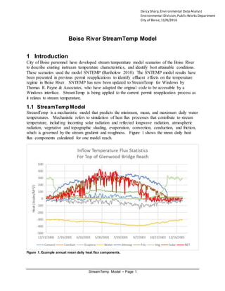
  • 1. StreamTemp Model – Page 1 Boise River StreamTemp Model 1 Introduction City of Boise personnel have developed stream temperature model scenarios of the Boise River to describe existing instream temperature characteristics, and identify best attainable conditions. These scenarios used the model SNTEMP (Bartholow 2010). The SNTEMP model results have been presented in previous permit reapplications to identify effluent effects on the temperature regime in Boise River. SNTEMP has now been updated to StreamTemp for Windows by Thomas R. Payne & Associates, who have adapted the original code to be accessible by a Windows interface. StreamTemp is being applied to the current permit reapplication process as it relates to stream temperature. 1.1 StreamTempModel StreamTemp is a mechanistic model that predicts the minimum, mean, and maximum daily water temperatures. Mechanistic refers to simulation of heat flux processes that contribute to stream temperature, including incoming solar radiation and reflected longwave radiation, atmospheric radiation, vegetative and topographic shading, evaporation, convection, conduction, and friction, which is governed by the stream gradient and roughness. Figure 1 shows the mean daily heat flux components calculated for one model reach. Figure 1. Example annual mean daily heat flux components. Darcy Sharp,Environmental Data Analyst Environmental Division,PublicWorks Department City of Boise; 11/8/2016
  • 2. StreamTemp Model – Page 2 Positive heat flux components are a heat gain to the system and negative components are heat loss from the system. These components illustrate the driving forces in heating and cooling. 1.2 TemperatureCriteria The 2016 StreamTemp model predicts the Boise River thermal response under alternative scenarios to help identify and interpret:  The proportion of the thermal load that is due to effluent flows and temperatures  Potential thermal load offset quantification Lander Water Renewal Facility (WRF) and West Boise WRF discharge to assessment unit (AU) ID17050114SW005_06, the reach from Veterans Memorial Parkway to Star Bridge. This AU is listed as impaired for temperature (DEQ 2014) These AUs are designated for the beneficial uses of Cold Water Aquatic Life (CWAL), Salmonid Spawning (SS) and Primary Contact Recreation. Temperature criteria that apply to these AUs include:  The CWAL criteria in IDAPA 58.01.02.250.02.b: “Water temperatures of twenty-two (22) degrees C or less with a maximum daily average of no greater than nineteen (19) degrees C.”  The site-specific SS criteria in IDAPA 58.01.02.278: “A maximum weekly maximum temperature of thirteen degrees C (13°C) to protect brown trout, mountain whitefish, and rainbow trout spawning and incubation applies from November 1 through May 30.”  IDAPA 58.01.02.010.59. Maximum Weekly Maximum Temperature (MWMT). “The weekly maximum temperature (WMT) is the mean of daily maximum temperatures measured over a consecutive seven (7) day period ending on the day of calculation. When used seasonally, e.g. spawning periods, the first applicable WMT occurs on the seventh day into the time period. The MWMT is the single highest WMT that occurs during a given year or other period of interest, e.g., a spawning period.” According to a memo referenced in Appendix E of the draft Third Edition of the Idaho Department of Environmental Quality Water Body Assessment Guidance (DEQ 2016), the following procedures apply to determination of temperature impairment:  The time period of interest to gage frequency of exceedance for CWAL temperature criteria is the 93-day period of June 21st through September 21st  If the frequency of exceedance is less than 10%, DEQ has the discretion to determine there is no impairment for temperature 2 Methods This section describes the steps used in setting up, calibrating, and running the StreamTemp model for the Boise River. Model extent and data sources are described.
  • 3. StreamTemp Model – Page 3 2.1 ModelSetup and Data Sources The model is initialized by entering the time records and dates for each model run. Annual daily records (January 1 to December 31) are selected for the Boise River model. Having an annual output of daily predictions allows interpretation of results on a seasonal, monthly, or weekly basis as needed. Regulatory issues may require evaluation of winter as well as summer limits. 2.1.1 Network Design The spatial extent of the StreamTemp model is from Lucky Peak to Middleton (Figure 2). The study reach includes the following AUs listed for temperature:  ID17050114SW005_06, extending from Veteran’s to Star  ID17050114SW005_06a, extending from Star to Middleton Figure 2. Spatial extent of StreamTempmodel of Boise River. The network design data entry includes a node title, location, and elevation at the top and bottom of each reach. StreamTemp automatically calculates the distance between nodes and the azimuth of the reaches. Table 1 provides the data entered in the network design screen. Table 1. Network design parameters for Boise River StreamTempmodel. Node Title Elevation (ft) Latitude Longitude Lucky Peak 2815 43.5378 -116.0934 Diversion Dam 2756 43.5652 -116.1319 Suez Water 2726 43.5833 -116.1606 Marden Footbridge 2684 43.6055 -116.2035 Veteran’s Bridge 2654 43.6364 -116.2430 Lander WRF 2611 43.6386 -116.2443 Glenwood Bridge 2595 43.6673 -116.2994 Loss to North Channel 2581 43.6719 -116.3265 West Boise WRF 2569 43.6729 -116.3317 Eagle Bridge South Channel 2520 43.6740 -116.4080 Gain from N Channel and Star 2472 43.6813 -116.4898 Middleton Gage 2411 43.6870 -116.5868 End 2405 43.6780 -116.5944
  • 4. StreamTemp Model – Page 4 A proportional schematic of the network design is shown in Figure 3. The view has been rotated 30° to ensure legibility of the labels. Figure 3. Schematic of the model reaches for Boise River StreamTempmodel. The south channel is simulated in the model network, but the north channel is not. Instead, the north channel is accounted for by streamflow loss and gain in the appropriate model reaches. 2.1.2 Reach Physical Geometry The reach physical geometry input screen includes azimuth, latitude, friction coefficients, width constant and coefficient, and thermal gradient coefficient. Typically, geometry analyses will include rating curves developed from channel measurements. Rating curves generally follow the format: 𝑈 = a𝑄 𝑏 and 𝐻 𝑜𝑟 𝑊 = α𝑄 𝛽 ,
  • 5. StreamTemp Model – Page 5 where U and H are velocity and height (or width) and where a, b, α, and β are empirical coefficients that are determined from velocity-discharge and stage-discharge rating curves, respectively. However, there are not enough existing channel data to develop rating curves for this temperature analysis. StreamTemp uses width constants and coefficients to describe channel geometry. Without channel measurements to develop rating curves, the width constant can be used to describe the width of the channel and the coefficient can be left at zero. The disadvantage of this method is that the physical geometry must be re-calibrated for each hydrologic scenario. The following figures show the difference between using a width coefficient and setting this coefficient to zero. Figure 4. Channel geometry of Veteran’s Bridge reach with V-shaped channel described by width constant and coefficient. Figure 5. Channel geometry of Veteran’s Bridge reachwith square channel described by width constant alone. StreamTemp is not a hydrology model, but it accounts for a water balance in each model reach. The size and shape of the channel affects the depth of the given streamflow. The same volume
  • 6. StreamTemp Model – Page 6 of water in a flat, broad channel will be warmer than in a narrow, V-shaped channel since more surface area is exposed to incoming solar radiation. The higher water column has a buffering effect on temperature extremes. This effect was apparent during temperature calibration of the Boise River scenarios. Simulating a V-shaped channel geometry smoothed the daily temperature predictions in the winter, but the actual monitoring data was showing large daily fluctuations. By applying the square-sided channels throughout the model reaches, temperature predictions became more accurate and were able to match the daily fluctuations in the winter. Table 2 provides the reach geometry parameters used for the calibrated existing conditions model. Table 2. Reach geometry worksheet from calibrated model. Reach Name Azimuth (degrees) Friction Coefficient (unitless) Width Constant (feet) Width Coefficient Thermal Gradient Lucky Peak 313.71 0.0430 100 0 1.65 Diversion Dam 310.35 0.0430 150 0 1.65 Suez Water 304.9 0.0350 59 0 1.65 Marden 316.63 0.0350 186 0 1.65 Veterans 335.16 0.0350 390 0 1.65 Lander WRF 310.69 0.0430 275 0 1.65 Glenwood Bridge 282.65 0.0300 62 0 1.65 Loss to North Channel 284.54 0.0350 83 0 1.65 West Boise WRF 270.70 0.0350 104 0 1.65 EagleSouth Channel 306.85 0.0350 117 0 1.65 Gain from North Channel 274.34 0.0350 139 0 1.65 Middleton Gage 269.52 0.0350 169 0 1.65 2.1.3 Hydrology Data The USGS 13202000 “Boise River nr Boise ID” streamgage is just downstream of Lucky Peak and represents the headwaters of the study reach. This streamgage has an extensive period of record of discharge measurements from 1895 through 2016. However, a water management agreement was reached in the Boise River valley starting on March 12, 1982 (U.S. Bureau of Reclamation 1984). The discharge measurements from this date through 2016 will be used to represent current hydrological conditions. The flow duration curve for current water management is shown in Figure 6. The 95th percentile low flow is 150 cubic feet per second (cfs), which means that 95% of the daily average streamflow records have been higher than 150 cfs. The 75th percentile flow is 250 cfs. This has typically been the streamflow from November through March, as shown in the discharge record in Figure 7.
  • 7. StreamTemp Model – Page 7 Figure 6. Flow duration curve for USGS 13202000 from March 1, 1982 through 2016 for current water management. Figure 7. Daily average streamflow at USGS 13202000 from March 1, 1982 through 2016. The streamgage USGS 13206000 “Boise River at Glenwood Bridge nr Boise ID” is between Lander and West Boise. The flow duration curve is provided in Figure 8.
  • 8. StreamTemp Model – Page 8 Figure 8. Flow duration curve at Glenwood from March 1, 1982 through August 22, 2016. The USGS 13206305 Boise River South Channel at Eagle ID is downstream of West Boise. The flow duration curve for this location is provided in Figure 9. The Glenwood and Eagle streamflow records were used to correct the water balance in the middle and near the end of the temperature study reach. Figure 9. Flow duration curve at Eagle from November 1, 1999 through August 22, 2016.
  • 9. StreamTemp Model – Page 9 Note that this streamgage has a shorter record of operation, beginning in 1999. 2.1.3.1 Selection of Representative Flow Years The temperature study is based on an extreme low flow scenario which represents the most critical conditions, and a median flow year which represents typical current conditions. The 95th percentile low flow 150 cfs occurred most frequently in 1983, but Boise City stream temperature monitoring dates back to 2000. In this timeframe, low flows of 152 and 153 cfs occurred during calendar years 2001 and 2002. Examining 2001 and 2002 weather data from the Boise AgriMet station for the warmest conditions shows that 2001 had 84 days where the maximum temperature was greater than 86°F, which is the temperature that stresses plant growth. In comparison, 2002 only had 34 days >86°F. See Table 3 for a brief data summary of air temperatures in 2001 and 2002. Table 3. Summary of air temperatures at Boise AgriMet weather station for 2001 and 2002. Air Temperature Parameter 2001 2002 Maximum daily mean (°F) 85 89 Maximum daily maximum(°F) 102 99 Days maximum temperature >86(°F) 84 34 The weather in 2001 presented more heat stress factors, so that is the year selected to represent the 95th percentile low flow scenarios. The annual flow record for this year is used to represent the headwaters of this scenario. To represent more typical hydrology, 2014 is chosen as a median flow year. The 75th percentile flow released from Lucky Peak Dam is 250 cfs. This has typically been the streamflow from November through March under the 1982 water management agreement. 2.1.3.2 Hydrology Data Entry The StreamTemp hydrology data screen provides options for each reach to include diversion, point or return flows. Streamflow data from USGS 13202000 and temperature data from Boise City are entered at the top reach. The Idaho Department of Water Resources (IDWR) accounts for diversion and return flows. Water rights accounting data is found at https://maps.idwr.idaho.gov/qWRAccounting/. Table 4 documents the location and data sources for hydrology and stream temperature, with river mile defined from Boise River confluence with Snake River to the upstream location. Table 4. Data sources and location for StreamTemphydrology. River Streamflow US Geological Survey (USGS) and Idaho Department of Water Resources (IDWR) Stations River Mile USGS 13202000 Boise River nr BoiseID 63.6 USGS 13206000 Boise River at Glenwood Bridge nr Boise ID 47.7 USGS 13206305 Boise River SouthChannel at Eagle ID 42.8 USGS andIDWR 13210050 Boise River nr Middleton ID 31.4 Diversion Hydrology IDWR station with discharge data 13202011 DiscoveryPark 63.3 13202995 PenitentiaryCanal 61.2 13203000 New York Canal below DiversionDam 61.2 13203600 Boise River below DiversionDam 61.1
  • 10. StreamTemp Model – Page 10 13203527 Surprise Valley/Micron 60.6 13203715 Shakespeare Festival 58.8 13203760 Ridenbaugh Canal 58.3 13203781 Williams Park 58.0 13204005 Bubb Canal 57.5 13204015 Herrick 57.1 13204020 Meeves Canal 56.8 13204060 Rossi Mill Canal 56.4 13204200 UnitedWater (Now Suez) 56.1 13204190 Boise CityCanal 55.9 13205514 Kathryn Albertson 52 13205515 Settlers Canal 52 13205517 FairviewAcres 51.8 13205613 Boise CityParks 51.5 13205622 Thurman Mill Canal 51.1 13205617 Drainage District #3 51 13205640 Farmers UnionCanal 50.4 13205642 Boise River at Veteran’s MemorialPark 50.2 13205984 Riverside Village 47.8 13206000 Boise River at Glenwood Bridge 47.7 13206090 New DryCreek Canal 45.6 13206096 Woods 45 13206205 Lemp Canal 44.8 13206220 Warm Springs Canal 44.5 13206270 Conway-Hamming Canal 43.5 13206290 Thomas AikenCanal 43.1 13206292 Mace-CatlinCanal 43.1 13206260 Graham-Gilbert Canal 42.9 13208738 Barber Pumps 42.4 13208740 Seven Suckers Canal 42 13209450 Thurman Drain 41.9 13209480 Phyllis Canal 41.4 13209990 Canyon CountyCanal 36.3 13210005 Caldwell Highline Canal 36.3 13210012 Otter Mitigation 35.7 River Temperature City of Boise BR07 LuckyPeak 63.6 BR06 Marden Footbridge 54.8 BR05 Veteran’s Memorial ParkBridge 50.2 BR04 GlenwoodBridge 47.7 BR03 Eagle Bridge southchannel 42.8 BR02 Middleton 31.4 Facility Volume and Temperature City of Boise Lander Water RenewalFacility 50 West Boise Water RenewalFacility 44.2 Locations for the 39 diversions and monitoring sites are shown in Figure 10.
  • 11. StreamTemp Model – Page 11 Figure 10. StreamTempmodel extent and data sources. The key input features in each of the model reaches are shown in Table 5. This table shows where the diversions are withdrawn from each model reach. Table 5. StreamTempmodel reachdescriptions. Model Reach River Mile Reach Name Data Source Name and USGS or IDWR Site Number City of Boise Stream and Effluent Temperature 1 63.6 to 61.2 LuckyPeak LuckyPeak, DiscoveryPark, PenitentiaryCanal 2 61.1 to 58.3 DiversionDam New York Canal, Surprise Valley/Micron, Shakespeare Festival, Ridenbaugh 3 58.2 to 56.1 Suez Water Williams Park, Bubb, Herrick, Meeves, Rossi, Suez 4 56.0 to 53.1 Marden Footbridge Boise CityCanalwithdrawal andMarden sampling location 5 53.0 to 50.1 Veteran’s Bridge Settler’s, Kathryn Albertson, Fairview Acres, Boise City Parks, ThurmanMill, Farmer’s Union, Veteran’s sampling location 6 50.0 to 47.9 Lander WRF Lander input 7 47.8 to 45.6 Glenwood Bridge Riverside Village, Glenwood samplinglocation, NewDryCreek Canal 8 45.5 to 44.5 Loss to North Channel Loss to North Channel, Woods. LempCanal, Warm Springs Canal 9 44.4 to 43.6 West Boise WRF West Boise input
  • 12. StreamTemp Model – Page 12 10 43.5 to 40.1 Eagle Bridge South Channel Conway-Hamming, Thomas Aiken, Mace-Catlin, Graham-Gilbert, Barber Pumps, Seven Suckers andPhyllis Canal withdrawals;ThurmanDraininputs;Eagle Bridge sampling location 11 40.2 to 36.4 Gainfrom North Channel Gainfrom NorthChannel to 1321000--Boise River near Star 12 36.3 to 31.1 Middleton Gage Canyon CountyCanal, Caldwell Highline Canal, Otter withdrawal; 13210050 Boise River near Middleton 13 31.0 End 2.1.4 Weather Data StreamTemp requires average air temperature, humidity, percent sunshine, wind speed and solar radiation to simulate stream temperatures. The weather data entry screen also requires the latitude and station elevation to calculate adiabatic lapse rate changes for stream reach elevations. There are also options for setting global constants and coefficients to describe local climate. The Boise AgriMet weather station at http://www.usbr.gov/pn/agrimet/webarcread.html provided the meteorology data for the Boise River temperature model. Although StreamTemp can calculate low and high air temperatures from average data, the Boise AgriMet station provided minimum and maximum daily air temperatures along with daily average. Having real data for the minimum and maximum air temperatures improved the calibration. The global constants and coefficients were left at default. 2.1.5 Shade Data For shade input parameters, the user can input percent shade if that value is known, or StreamTemp will calculate percent shade from reach azimuth, total stream corridor width, vegetation offset, and topographic shade. Temperature predictions improved slightly when StreamTemp was allowed to automatically fill percent shade values that varied daily for each model reach. Final parameters used by the model to calculate shade are shown in Table 6. Table 6. Parameters usedto calculate daily average shade. Reach Name Stream Corridor Width (ft) Vegetation Offset (ft) Left Bank Right Bank LuckyPeak 547.43 223.71 223.71 Diversion Dam 547.43 198.71 198.71 Suez Water 980.68 460.84 460.84 Marden 547.43 180.71 180.71 Veterans 547.43 78.71 78.71 Lander WRF 547.43 136.21 136.21 GlenwoodBridge 547.43 242.71 242.71 Loss to NorthChannel 547.43 232.21 232.71 West Boise WRF 547.43 221.71 221.71 Eagle SouthChannel 547.43 215.21 215.21 Gainfrom NorthChannel and Star 547.43 204.21 204.21 MiddletonGage 547.43 189.21 189.21 2.2 Calibration Once all of the input variables were entered into the worksheets and the best literature values and equations were selected, the model was run and output compared to existing data. This process is
  • 13. StreamTemp Model – Page 13 used to calibrate the model to ensure accurate modeled stream temperatures. Error statistics are reported as bias--based on the difference of the residuals--and root mean squared error (RMSE). 2.2.1 2014 Median Flow Hydrology The following description documents the steps taken to calibrate model predictions to monitoring data. The StreamTemp model does not simulate hydrology, but it checks the water balance for each model reach. The inputs for the Lucky Peak reach are streamflow from USGS 13202000 and temperature from Boise City’s Lucky Peak monitoring location. The first model reach with existing temperature data is at the Marden Footbridge. The model predictions were compared to the 2014 Boise City stream temperature data as shown in Figure 11 and Figure 12. Error statistics describe prediction error and model performance. The difference between values predicted by a model and the sample data are called residuals. The goal of calibration is to reduce the residuals as much as possible. The error statistics chosen for this report are bias and root mean squared error (RMSE). Bias subtracts each daily average measurement from each daily average prediction and finds the difference. This is the average mean error, or bias, since it also shows whether the prediction is above or below the measured data on average. The RMSE takes the square of each daily average difference, sums those squares and divides by the number of records, then takes the square root of this sum. The practical application of these error statistics is that the bias averages the residuals, and the RMSE emphasizes the outliers of the residuals. In the Marden comparison in Figure 11, the residuals are greatest in the winter months, so the RMSE is 0.42°C, whereas the overall bias of the prediction is -0.08°C. Whereas bias and RMSE describe the magnitude of the residuals, correlation describes how well one array compares to another, in this instance, the time series of measured to modeled data. When comparing one array to another, a 1.0 with an intercept of zero would be a perfect correlation. The correlation in Figure 12 is 0.9939.
  • 14. StreamTemp Model – Page 14 Figure 11. Comparison of daily average measuredand modeled stream temperature at Marden Footbridge. Figure 12. Correlation of daily average measuredto modeled stream temperature at Marden Footbridge. Veteran’s Bridge is the next model reach with monitoring data to check the calibration. Model performance is shown in Figure 13 and Figure 14.
  • 15. StreamTemp Model – Page 15 Figure 13. Comparison of daily average measuredand modeled stream temperature at Veteran’s Bridge. Figure 14. Correlation of daily average measuredto modeled stream temperature at Veteran’s Bridge.
  • 16. StreamTemp Model – Page 16 Note that the biggest discrepancy in model prediction is mid-November, when measured temperature dropped to 3.86°C. Presumably, this drop in temperature was a response to a failure at Diversion Dam resulting in streamflow dropping to 8 cfs on 10/22/2014. Flow increased to 250 cfs, the 75th percentile low flow, for the rest of the year, but the streamflow shutdown apparently caused a decreased temperature signal that passed through the rest of the river. The model tended to have more difficulty fitting this abrupt temperature drop. For the Veteran’s Bridge reach, the overall bias of the model over predicts by +0.19°C with RMSE=0.81°C. The correlation is 0.9766. The Glenwood Bridge reach includes existing data from Boise City temperature and USGS streamflow. The streamflow records were used to correct the water balance. Water volume at this point is a function of headwaters inflow with diversion outflow. The difference between this calculated volume with actual volume is due to evaporation, groundwater returns and withdrawals, and undocumented consumption. Figure 15 and Figure 16 display the model predictions compared to measured data for temperature. Figure 15. Comparison of daily average measuredand modeled stream temperature at Glenwood Bridge. Again, notice the same drop in temperature in mid-November as seen in the Veteran’s reach.
  • 17. StreamTemp Model – Page 17 Figure 16. Correlation of daily average measuredto modeled stream temperature at Glenwood Bridge. For the Glenwood Bridge reach, the overall bias of the model underpredicts by 0.08°C with RMSE=0.62°C. The correlation is 0.9844. Eagle Bridge in the Boise River south channel is the next model reach with existing data from Boise City temperature and USGS streamflow. The streamflow records were used to correct the water balance. Figure 17 and Figure 18 display the model predictions compared to measured data for temperature.
  • 18. StreamTemp Model – Page 18 Figure 17. Comparison of daily average measuredand modeled stream temperature at Eagle Bridge. Figure 18. Correlation of daily average measuredand modeled stream temperature at Eagle Bridge. For the Eagle Bridge reach, the overall bias of the model overpredicts by 0.03°C with RMSE=0.50°C. The correlation is 0.9893.
  • 19. StreamTemp Model – Page 19 Altering channel widths to account for ponds adjacent to the river channel proved to be the best calibration tool for reducing the residuals in the stream temperature record. When channel widths increased, the variability in winter temperatures was easier to simulate. With winter low flows and a wide channel, a shallow water column allows for less insulating potential. With less insulating potential, there is a more rapid stream temperature response to atmospheric temperatures. This is exemplified in the measured air and stream temperature records at Marden (Figure 19). Figure 19. Stream temperatures show a quicker response to air temperatures at low flow. During winter low flows averaging 250 cfs, the stream temperature responds to a drop in air temperature within one day or less. Note the data callouts for February 6th and 7th and for November 18th. However, for the July high air temperature which occurred on July 14th, the stream temperature response occurred 46 days later. Streamflows ranged from 1834 cfs to 928 cfs during this time. These data illustrate the insulating properties of a greater depth of water in the channel. 2.2.2 2001 95th Percentile Low Flow Hydrology Once the 2014 median flow year was calibrated, the 2001 95th percentile low flow year was calibrated. Using the same data sources as shown above in Table 4, the meteorology,
  • 20. StreamTemp Model – Page 20 streamflow, and stream temperature records for 2001 were entered into StreamTemp. The following figures document the error statistics for the 2001 low flow hydrology scenario. Figure 20. Comparison of daily average measuredand modeled stream temperature at Veteran’s Bridge. Figure 21. Correlation of daily average measuredand modeled stream temperature at Veteran’s Bridge.
  • 21. StreamTemp Model – Page 21 Figure 22. Comparison of daily average measuredand modeled stream temperature at Glenwood Bridge. Figure 23. Correlation of daily average measuredand modeled stream temperature at Glenwood Bridge.
  • 22. StreamTemp Model – Page 22 Figure 24. Comparison of daily average measuredand modeled stream temperature at Eagle Bridge. Figure 25. Correlation of daily average measuredand modeled stream temperature at Eagle Bridge.
  • 23. StreamTemp Model – Page 23 Table 7 provides a summary of the error statistics for the 2014 median hydrology model and the 2001 low flow hydrology model. Table 7. Temperature error statistics summary. Model Monitoring location Bias (°C) RMSE (°C) Correlation (R2) 2014 median hydrology Marden Footbridge -0.08 0.42 0.9939 Veteran’s Bridge +0.19 0.81 0.9766 GlenwoodBridge -0.08 0.62 0.9844 Eagle Bridge southchannel +0.03 0.50 0.9893 2001 low flow hydrology Veteran’s Bridge +0.12 0.31 0.9979 GlenwoodBridge +0.28 0.55 0.9932 Eagle Bridge southchannel +0.14 0.58 0.9892 A typical goal of modeling stream temperatures is to accurately predict temperature within ±1°C. The StreamTemp model performance shows overall bias of less than 0.3°C. 3 Results Model scenarios describing alternative WRF operation are developed to identify effluent effects on the temperature regime in Boise River. Model results identify:  The proportion of the thermal load that is due to effluent flows and temperatures  Potential thermal load offset projects 3.1 Alternative managementscenarios 3.1.1 Descriptions Scenarios developed for the permit reapplication compare WRF effects with existing effluent flow and temperature, with design flows, and with no effluent flows to the river. Further scenarios show the effect of the Lander effluent discharging to Farmer’s Union Canal from April 1st through November 31st. The “2001 hydrology” scenarios are based on 95th percentile low flow to illustrate critical conditions. The “2014 hydrology” scenarios are based on median hydrology for typical conditions. Scenario I: 2001 hydrology—Both WRF, actual effluent flow and temperature This is existing stream morphology and hydrology—including current water management inputs and withdrawals—temperature, climate, and shade conditions for January 1 through December 31, 2001. Scenario II: 2001 hydrology—Lander to Farmer’s Union, actual effluent flow and temperature With the other parameters remaining constant to Scenario I, the flow at Lander is set at zero from April 1 through November 31 when Boise City has an agreement with Farmer’s Union Irrigation District to divert all of the effluent flow to the canal. Scenario III: 2001 hydrology—No WRF
  • 24. StreamTemp Model – Page 24 With the other parameters remaining constant to Scenario I, no point source flow and temperature were added in the Lander or West Boise model reaches. This scenario shows what effect removing the effluent flow would have on a low flow year. Scenario IV: 2001 hydrology—Both WRF, design effluent flow and high temperature Critical conditions are expressed by 95th percentile low flow hydrology and both WRFs set at design flow, which is 23 cfs per day at Lander and 37 cfs per day at West Boise. The 2015 temperatures for these facilities were entered because that was the warmest effluent year on record. Scenario V: 2001 hydrology—Lander to Farmer’s Union, design effluent flow and high temperature With the other parameters remaining constant to the Scenario IV design effluent flow and high temperatures, the flow at Lander is set at zero from April 1 through November 31. Scenario VI: 2014 hydrology—Both WRF, actual effluent flow and temperature This is existing stream morphology and hydrology—including current water management inputs and withdrawals—temperature, climate, and shade conditions for January 1 through December 31, 2014. Scenario VII: 2014 hydrology—Lander to Farmer’s Union, actual effluent flow and temperature With the other parameters remaining constant to Scenario VI, the flow at Lander is set at zero from April 1 through November 31 when Boise City has an agreement with Farmer’s Union Irrigation District to divert all of the effluent flow to the canal. Scenario VIII: 2014 hydrology—No WRF With the other parameters remaining constant to Scenario VI, no point source flow and temperature were added in the Lander or West Boise model reaches. This scenario shows what effect removing the effluent flow would have on a median flow year. Scenario IX: 2014 hydrology—Both WRF, design flow and high temperature Both WRFs are set at design flow, which is 23 cfs per day at Lander and 37 cfs per day at West Boise. The 2015 temperatures for these facilities were entered because that was the warmest effluent year on record. Scenario X: 2014 hydrology—Lander to Farmer’s Union, design flow and high temperature With the other parameters remaining constant to the Scenario IX design effluent flow and high temperatures, the flow at Lander is set at zero from April 1 through November 31.
  • 25. StreamTemp Model – Page 25 3.1.2 Alternative management scenario results Daily average and daily maximum predicted temperatures for the ten alternative management scenarios were compared to the applicable criteria in Idaho’s Water Quality Standards:  The CWAL criteria in IDAPA 58.01.02.250.02.b: “Water temperatures of twenty-two (22) degrees C or less with a maximum daily average of no greater than nineteen (19) degrees C.”  The site-specific SS criteria in IDAPA 58.01.02.278: “A maximum weekly maximum temperature of thirteen degrees C (13°C) to protect brown trout, mountain whitefish, and rainbow trout spawning and incubation applies from November 1 through May 30.” According to a memo referenced in Appendix E of the draft Third Edition of the Idaho Department of Environmental Quality Water Body Assessment Guidance (DEQ 2016), the following procedures apply to determination of temperature impairment:  The time period of interest to gage frequency of exceedance for CWAL temperature criteria is the 93-day period of June 21st through September 21st  If the frequency of exceedance is less than 10%, DEQ has the discretion to determine there is no impairment for temperature Figure 26 and Figure 27 show monthly average stream temperatures predicted for the ten alternative management scenarios compared to CWAL and SS criteria. Figure 26. Monthly average predicted stream temperatures at Lander compared to criteria.
  • 26. StreamTemp Model – Page 26 Figure 27. Monthly average predicted stream temperatures at West Boise comparedto criteria. The CWAL period is 93 days from June 21 through September 21 and the SS period is 207 days from November 1 through May 30. In low flow years, there are some monthly average exceedances in August, but none in median flow years. Table 8 shows the daily percent exceedances for the applicable criteria. The results are reported for the river model reach downstream of Lander and West Boise WRFs. Table 8. Percent exceedances of applicable temperature criteria in river reachdownstream of each W RF. Lander West Boise CWAL Max CWAL Avg SS CWAL Max CWAL Avg SS Scenario I--2001 hydrology--Both WRF, actual effluent flow and temperature 0 46.2 0 4.3 48.4 0 Scenario II--2001 hydrology—Lander to Farmer’s Union, actual effluent flow and temperature 0 31.2 0 1.1 38.7 0 Scenario III--2001 hydrology—No WRF 0 31.2 0 1.1 35.5 0 Scenario IV-2001 hydrology—Both WRF, design effluent flow and high temperature 0 38.7 0 4.3 50.5 5.8 Scenario V—2001 hydrology—Lander to Farmer’s Union, design effluent flow and high temperature 0 31.2 0 4.3 47.3 5.8 Scenario VI—2014 hydrology—Both WRF, actual effluent flow and temperature 0 0 4.3 0 0 3.4
  • 27. StreamTemp Model – Page 27 Scenario VII—2014 hydrology—Lander to Farmer’s Union, actual effluent flow and temperature 0 0 2.9 0 0 3.4 Scenario VIII—2014 hydrology—No WRTF 0 0 2.9 0 0 2.9 Scenario IX—2014 hydrology—Both WRF, design flow and high temperature 0 0 4.3 0 0 5.3 Scenario X—2014 hydrology—Lander to Farmer’s Union, design flow and high temperature 0 0 2.9 0 0 4.3 The scenarios for the 95th percentile low flow year describe critical conditions. For 2001 hydrology, the CWAL average criterion are exceeded, with or without effluent flows, but the CWAL maximum criterion is not exceeded more than 10% of the time. It is interesting that the percent exceedances for the design flow scenario (Scenario IV) are fewer than current conditions at Lander. This is due to the added volume of water, which insulates the stream from rapid heat exchange with the atmosphere. The SS MWMT criterion is exceeded 5.8% of the time at West Boise when it is at design flow. If the frequency of exceedance is less than 10%, DEQ has the discretion to determine there is no impairment for temperature. For the scenarios with median flow conditions, the CWAL criteria are never exceeded, with or without effluent flows. Depending on the scenario, the SS MWMT criterion is exceeded from 2.9% to 5.3% of the time, which is still less than the 10% exceedance threshold. The extra volume of water in the winter allows more insulation from cold air temperature. The reason that the SS criterion is not exceeded during low flow hydrology is that there is not enough flow in the channel to insulate from cold air temperatures. With effluent flow from West Boise removed, the south channel freezes over some days in the winter—the stream temperature record goes to zero in December. Volume and temperature are inversely related. Modeled existing conditions for 2001 low flow hydrology show that when streamflow is higher in June and July, temperatures are lower than later in the season. During September, streamflows are lower and temperatures are higher (Figure 28). The lower water volume has less insulating effect and there is a more rapid response to temperature changes. Modeled existing conditions for 2014 median flow hydrology also show an inverse relationship between stream volume and temperature, but the response time lags compared to low flows (Figure 29).
  • 28. StreamTemp Model – Page 28 Figure 28. Modeled existing conditions for 2001 low streamflow hydrology shown for CWAL period. Figure 29. Modeled existing conditions for 2014 median streamflow hydrology shown for CWAL period.
  • 29. StreamTemp Model – Page 29 Because of the insulating effect of higher water volume, the average stream temperature is 18.1°C between Lander and West Boise during low flows, but 16.6°C during median flows. The following table and figure further demonstrate the relationship between temperature and streamflow for the model scenarios. Table 9. Seasonal average temperature and streamflow for CWAL period for each model scenario. Figure 30. Seasonal average streamflow and temperature for the ten model scenarios. 3.1.3 WRF thermal contribution calculations Since the CWAL average criterion would be exceeded during low flow years, the proportion of the excess heat load in the river that is due to effluent is evaluated for the CWAL period from Average Temperature (°C) Average Streamflow (cfs) Average Temperature (°C) Average Streamflow (cfs) Scenario I-Both WWTFs-Actual 18 680 18.2 617 Scenario II-Lander to Farmer's Union, Actual 17.7 659 17.9 596 Scenario III-No WWTFs 17.7 659 17.8 576 Scenario IV-Both WWTFs-Design 17.9 682 18.3 637 Scenario V-Lander to Farmer's Union, Design 17.7 659 18.2 613 Scenario VI-Both WWTFs-Actual 16.3 1292 16.8 1218 Scenario VII-Lander to Farmer's Union, Actual 16.2 1274 16.7 1199 Scenario VIII-No WWTFs 16.2 1274 16.6 1174 Scenario IX-Both WWTFs-Design 16.3 1297 16.9 1234 Scenario X-Lander to Farmer's Union, Design 16.2 1274 16.8 1211 2001LowFlow Hydrology 2014MedianFlow Hydrology Lander West Boise
  • 30. StreamTemp Model – Page 30 June 21 through September 21. Subtracting the daily average stream temperature of one scenario from another can help identify the thermal contribution of the facilities under alternative scenarios. Boise City has an agreement with Farmer’s Union Canal District where all of the effluent from Lander WRF may be discharged to the canal from April 1 through November 30 each year. This is the long term plan of operations. Critical conditions are expressed by using 95th percentile low flow hydrology and both WRFs set at design flow, which is 23 cfs per day at Lander and 37 cfs per day at West Boise with 2015 temperatures for these facilities because that was the warmest year for effluent. Figure 31 shows the difference between existing conditions and design flows at the WRFs with Lander discharging to Farmer’s Union April 1 through November 31. Figure 31. Predicted daily average temperature difference betweenexisting conditions and a scenariowith both facilities at design flow, but Lander discharging to Farmer’s Union Canal—2001 low flow hydrology. In the river just downstream of the Lander outfall, existing conditions average 0.3°C warmer than the scenario where Lander discharges to Farmer’s Union because of the volume of flow that is diverted. In the river just downstream of the West Boise outfall, existing conditions average 0.07°C warmer than the Lander to Farmer’s Union scenario. However, from 9/7/2001 to 9/21/2001, existing conditions would be cooler because this is the timeframe when streamflow is so low—see Figure 28 above for temperature and hydrology comparison. If the existing agreement with Farmer’s Union Irrigation District does not come to pass, the critical condition of concern would be both WRFs at design flow. Figure 32 shows the predicted difference between design flow conditions and existing conditions.
  • 31. StreamTemp Model – Page 31 Figure 32. Predicted daily average temperature difference between design effluent at both facilities and existing conditions—2001 low flow hydrology. Temperatures in the river downstream of the Lander outfall are predicted to average 0.1°C cooler with existing conditions subtracted from design conditions. This indicated that additional flow volume is more important than any thermal impact during an extreme low streamflow year. In the river just downstream of West Boise with design effluent flows, stream temperatures are predicted to average 0.09°C warmer than existing conditions. This would be the thermal contribution of WRF operation during an extreme low streamflow year. For the 2014 median hydrology year, Figure 33 shows the difference between existing conditions and design flows at the WRFs with Lander discharging to Farmer’s Union April 1 through November 31. For this comparison, the average difference to stream temperature is 0.1°C downstream of the Lander outfall and 0.02°C in the West Boise reach—this would be the average thermal contribution offset for diverting effluent to the canal during a typical year. If the existing agreement with Farmer’s Union Irrigation District does not come to pass, the critical condition of concern would be both WRFs at design flow. Figure 34 shows the predicted difference between design flow conditions and existing conditions.
  • 32. StreamTemp Model – Page 32 Figure 33. Predicted daily average temperature difference betweenexisting conditions and a scenariowith both facilities at design flow, but Lander discharging to Farmer’s Union Canal—2014 median flow hydrology. Figure 34. Predicted daily average temperature difference betweendesign effluent at both facilities and existing conditions—2014 median flow hydrology.
  • 33. StreamTemp Model – Page 33 For the difference between design effluent and existing conditions, the average difference to stream temperature is 0.03°C downstream of the Lander outfall and 0.08°C in the West Boise reach. To summarize the results from these scenario comparisons, the occasions where WRF operations contribute a thermal load include:  West Boise with design effluent flows would contribute 0.09°C heat load to the river during an extreme low streamflow year  Lander at design flow would contribute 0.03°C to the river during a median flow year  West Boise at design flow would contribute 0.08°C to the river during a median flow year The thermal contribution can be converted from degrees Celsius to Million kilocalories (Mkcal) by the following conversion formula: Table 10 shows the thermal contribution in degrees as well as Mkcal for the differences between the scenarios that result in a positive heat load contribution to the river. Table 10. Thermal contribution for the differences between key scenarios. Thermal Contribution (°C) Design Flow (cfs) Thermal Contribution (Mkcal/day) Seasonal Thermal Contribution (Mkcal/CWAL Period) West Boiseat design flow--2001 hydrology 0.09 37 8.15 757.95 Lander at design flow--2014 hydrology 0.03 23 1.69 157.17 West Boiseat design flow--2014 hydrology 0.08 37 7.24 673.32 The seasonal thermal contribution is for the 93-day CWAL period. 3.2 Heat flux component low flow scenarios In order to compare the relative contribution of the heat load from effluent with other heat sources, twelve more scenarios were developed for the 95th percentile low flow year. 3.2.1 Scenario Descriptions Scenario 1: WRF-Existing Conditions This is existing stream morphology and hydrology—including current water management inputs and withdrawals—temperature, climate, and shade conditions for January 1 through December 31, 2001. 23 ft3 1 m3 1000 kg 86400 sec kcal 1 Million kcals 0.1 °C = 5.62946 Mkcal 1 sec 35.3 ft3 1 m3 1 day kg·°C 1000000 kcals day
  • 34. StreamTemp Model – Page 34 Scenario 2: No WRF-Existing Conditions With the other parameters remaining constant to Scenario 1, no point source flow and temperature were added in the Lander or West Boise model reaches. This scenario shows what effect removing the effluent flow would have on a low flow year. Scenario 3: WRF-100% Shade Same as Scenario 1, but with 100% shade cover at 100% density. Scenario 4: No WRF-100% Shade Same as Scenario 2, but with 100% shade cover at 100% density Scenario 5: WRF 30-foot channel, no diversions This scenario removes all withdrawals, diversions, and groundwater inflow or outflow. In addition, the channel geometry was set to 30-feet wide in all the model reaches. This evaluates the headwaters inflow volume and temperature as the water volume moves downstream in a uniform channel and begins to reach atmospheric thermal equilibrium. Scenario 6: No WRF 30-foot channel, no diversions Same as Scenario 5, but with no effluent flow volume or temperature inputs. Scenario 7: WRF, 50-foot channel, no diversions Same as Scenario 5, but with 50-foot wide channel in all reaches. Scenario 8: No WRF, 50-foot channel, no diversions Same as Scenario 6, but with 50-foot wide channel in all reaches. Scenario 9: WRF, 50-foot channel, no diversions, climate change 2040 Same as Scenario 7, but with climate change assumptions for the year 2040 added to the air temperature record. Scenario 10: No WRF, 50-foot channel, no diversions, climate change 2040 Same as Scenario 8, but with climate change assumptions for the year 2040 added to the air temperature record. Scenario 11: WRF, 50-foot channel, no diversions, climate change 2080 Additional heating for the year 2080 added to Scenario 7. Scenario 12: No WRF, 50-foot channel, no diversions, climate change 2080 Additional heating for the year 2080 added to Scenario 8. For climate change scenarios, most models use lower streamflow and higher air temperatures. Increased air temperatures affect the amount of water stored in the snowpack, since more precipitation will fall as rain rather than snow in winter. Without the snowpack, instream flows will be reduced. However, since Boise River is under a water management agreement (U.S. Bureau of Reclamation 1984) that leaves a 250 cfs baseflow in the river during the winter, the above climate change scenarios do not include any flow reduction. For air temperatures, climate simulation models predict an average 2.8°C increase from 2000 to 2050 (Mote 2001). The
  • 35. StreamTemp Model – Page 35 model input applied a 1°C air temperature increase to the 2001 daily record for the 2040 scenario and a 2°C increase for the 2080 scenario. 3.2.2 Heat flux component scenario results Differences among the 95th percentile low flow scenarios will help identify components of the heat load. The annual average of the 50th percentile temperature predictions for each scenario are displayed by model reach, or river mile. This will show how stream temperature trends away from baseline temperature and toward atmospheric temperatures in a downstream direction, and how different factors buffer or exacerbate this heat increase. The difference between scenarios with existing shade and scenarios with 100% shade density are shown in Figure 35. In this figure, the vertical gray lines equate with the StreamTemp model nodes, where river mile 14 is downstream of the Lander outfall, river mile 18 is downstream of the West Boise outfall, and river mile 26 is downstream of north channel returning to Boise River. Figure 35. Annual average stream temperatures comparing existing shade with 100% shade. In these scenarios, the annual average heat increase from Lucky Peak at the model headwaters to Middleton is:  WRF-Existing Shade=2.4°C  No WRF-Existing Shade=1.9°C  WRF-100% Shade=1.9°C  No WRF-100% Shade=1.5°C The differences between existing shade and 100% shade model inputs are shown in Figure 36.
  • 36. StreamTemp Model – Page 36 Figure 36. Existing shade and 100% shade StreamTempdata entry. Figure 36. Shade data input for existing shade and 100% shade. 100% shade provides 0.5°C annual average cooling over existing conditions. Boise River is in a wide floodplain-type channel where topographic and vegetative shade are less important cooling factors than channel pattern and morphology. To investigate the effects of the stream channel on heat flux, the morphology was simplified to thirty feet wide for the entire study reach; groundwater losses and gains were removed; and all diversions and drains were removed (Figure 37). Existingshade: • Calculates daily shade • Zero density 100% shade: • 100% daily shade • 100% density
  • 37. StreamTemp Model – Page 37 Figure 37. Annual average stream temperatures comparing channelized morphology with existing conditions. From comparing existing channel morphology with the theoretical 30-foot-wide channel, factors of heating and cooling are able to be isolated. The channelized scenario demonstrates:  A groundwater cooling effect between river miles 6 and 12  A heat source from gain from the north channel between miles 21 and 26  A heat gain in the West Boise model reach has a heat gain with or without effluent The heat gain in the West Boise reach in the absence of effluent is because the aspect of this model reach is due west, which has less potential to provide topographic or vegetative shade. StreamTemp heat flux output demonstrates the heat source due to aspect. In Figure 38, the factors above the x-axis are heat sources, and the factors below the x-axis are heat sinks.
  • 38. StreamTemp Model – Page 38 Figure 38. Heat flux parameters for low flow current conditions comparing Lander reachwith West Boise reach. The West Boise WRF is in a stream channel reach that faces due west. Particularly in the winter, this creates a lack of topographic or riparian shade that becomes a source of heat. Comparing the annual variation of heat fluxes for each model reach shows how channel morphology affects sources and sinks of heat. Climate change scenarios demonstrate that stream temperatures would be generally warmer throughout the river until the reach containing the gain from north channel (Figure 39). This shows that incoming stream temperatures in Boise River are more important than increased air temperatures as a heat source.
  • 39. StreamTemp Model – Page 39 Figure 39. Annual average stream temperatures comparing climate change with existing conditions. The above scenarios compare annual average stream temperatures with river mile for the 95th percentile low flow year. Using extreme low flow helps isolate heat flux components. Features of the river that affect heat load include:  Riparian and topographic shade  Azimuth of the model reach  Channel width  Diversions and returns (water volume)  Air temperatures  Inflowing stream temperatures Table 11 shows how the annual average stream temperature at Middleton would compare among these scenarios. Table 11. Annual average temperature at Middleton for heat flux component scenarios. Temperature at Middleton (°C) Scenario 11.72 Scenario 1 WRF-Existing Conditions 11.2 Scenario 2 No WRF-Existing Conditions 11.15 Scenario 3 WRF-100% Shade 10.79 Scenario 4 No WRF-100% Shade 10.55 Scenario 5 WRF 30-foot channel, no diversions 9.9 Scenario 6 No WRF 30-foot channel,no diversions 10.48 Scenario 7 WRF, 50-foot channel,no diversions 10.19 Scenario 8 No WRF, 50-foot channel, no diversions,
  • 40. StreamTemp Model – Page 40 11.04 Scenario 9 WRF, 50-foot channel,no diversions,climatechange2040 10.55 Scenario 10 No WRF, 50-foot channel, no diversions,climatechange2040 11.42 Scenario 11 WRF, 50-foot channel,no diversions,climatechange2080 11.02 Scenario 12 No WRF, 50-foot channel, no diversions,climatechange2080 From these annual average stream temperatures for existing conditions:  the north channel gain temperature increase is 0.85°C  the difference between current operations and removing the effluent is 0.52°C at Middleton  temperature increase at the West Boise reach due to aspect equals 0.10°C The other scenarios are extreme examples, including maximum shade and completely channelized stream conditions. For some of these scenarios, differences from existing conditions include:  0.93°C cooling from 100% shade  1.17°C cooling by decreasing the channel to 30-feet wide and removing diversions and withdrawals  2040 climate increases stream temperatures by 0.56°C  2080 climate increases stream temperatures by 0.94°C Riparian shade, channel width, water volume, and increasing air temperatures all have been altered by human influences to add heat load to the river. Inflowing stream temperatures have also been altered since the bottom withdrawal at Lucky Peak dam creates cooler headwaters temperatures than would occur without reservoir operation. Among all these human influences on stream temperature, only a proportion of the total excess heat load is the responsibility of WRF effluent. 3.3 Thermaloffset scenarios From the alternative management scenarios presented in Section 3.1, the WRF thermal contribution is 0.09°C at West Boise at low streamflow hydrology and 0.03°C at Lander and 0.08°C at West Boise for median streamflows. To evaluate riparian restoration projects that can alleviate the heat load, a thermal offset scenario was developed. The Boise City model analysis investigated the two river miles upstream of Lander in more detail using the 2014 hydrology and meteorology with modeled streamflow and measured stream temperatures at Veteran’s Bridge. This finer-scale model was set up with a model node every 0.10 river miles based on a contour layer with two-foot elevation intervals. See Figure 40 for the thermal offset scenario model nodes.
  • 41. StreamTemp Model – Page 41 Figure 40. Thermal offset study reach. Large ponds in Veteran’s Memorial Park adjacent to the river proved to be a heat source during the model calibration process. If a flow-through side channel were created from an adjacent pond, the potential surface area contributing heat load to the river could be reduced. Figure 41 is a visualization of where a new channel could be built. Figure 41. Visualization of flow-through side channel createdin a Veteran’s Park pond adjacent to Boise River.
  • 42. StreamTemp Model – Page 42 Selection of this location is also validated by examining 1939 aerial photography that showed the current location of these ponds was historically a braided stream (Figure 42). Figure 42. Aerial imagery from 1939 showing area currently occupied by ponds in Veteran’s Park. To simulate this restoration project, the existing conditions scenario included the entire width of the ponds, but the side channel scenario used channel widths just to the theoretical improvement. The highlighted cells in Table 12 show the changes in the side channel scenario. Table 12. Reach geometry width differences betweenexisting conditions model and side channel scenario. Node Azimuth (degrees) Manning’s N (friction coefficient) Existing Width Constant (feet) Side Channel Scenario Width Constant (ft) 1 304 0.0430 252 252 2 323.47 0.0430 276 276 3 304.01 0.0430 180 180 4 304.01 0.0430 204 204 5 359.47 0.0430 119 119 6 0.00 0.0430 126 126 7 359.47 0.0430 142 142 8 359.47 0.0430 143 143 9 359.47 0.0430 149 149 10 304.01 0.0350 192 192 11 323.48 0.0350 430 121 12 323.48 0.0350 646 356 13 339.52 0.0350 851 512 14 323.48 0.0430 569 368 15 323.49 0.0300 123 123 16 304.02 0.0350 92 92 17 359.48 0.0350 155 155 18 323.49 0.0350 110 110 19 304.03 0.0350 154 154
  • 43. StreamTemp Model – Page 43 Model results showed that with the addition of a side channel affecting 0.4 river miles, the temperature reduction from existing conditions averages 0.09°C June 21 – July 20, 0.11°C July 21-August 20, and 0.05 °C August 21 – September 21 (Table 13). June 21 through August 21 is the CWAL period when temperature exceedances would occur during critical flow conditions. Table 13. Monthly temperature reduction from creating a side channel at Veteran’s Bridge. Temperature Reduction (°C) Node June21 - July 20 Average July 21 - August 20 average August 21 - September21 average 11 0.02 0.03 0.01 12 0.04 0.05 0.03 13 0.07 0.10 0.04 14 0.09 0.12 0.05 15 0.09 0.11 0.05 16 0.09 0.11 0.05 17 0.09 0.11 0.05 18 0.09 0.11 0.05 19 0.09 0.11 0.05 If Lander’s thermal contribution is 0.03°C in a median flow year, this restoration project could offset the entire contribution. That would be in addition to the thermal contribution offset from Lander effluent being discharged to Farmer’s Union Canal from March 1 through November 31. This side channel restoration analysis quantifies the reduction in solar loading solely from a change in water surface area. If riparian shade and channel complexity are added to the side channel, these features would increase the thermal benefit. A mature, functioning vegetative canopy cover will further reduce the heat load to the stream by blocking incoming solar radiation from reaching the channel. 4 Discussion This study uses modeling to identify the stream temperatures that would result under alternative management scenarios at Lander and West Boise water renewal facilities. In addition, a wide range of scenarios isolated components of heat loading to the river such as air temperature, channel width, topographic and vegetative shade, groundwater temperature and discharge, facility water temperature and discharge, and tributary (North Channel) temperature and flow. The alternative management scenarios showed that during an extreme low flow year, the 19°C average CWAL criterion is exceeded, with or without WRF effluent inputs. A portion of the excess heat load that causes this exceedance is due to WRF effluent. StreamTemp is also able to demonstrate that other portions are due to channel geometry, ponds adjacent to the stream, aspect, and lack of topographic and riparian shade. Some of these features are natural (aspect and lack of topographic shade) and some of these features are due to human influences. Generally, stream temperature trends away from baseline temperature and toward atmospheric temperatures in a downstream direction. For the temperature study reach of the Boise River, the baseline temperature is that of the bottom release from the Lucky Peak Lake storage reservoir.
  • 44. StreamTemp Model – Page 44 Without insulating or buffering processes, the river would attain thermal equilibrium with atmospheric temperature dynamics. In general, stream characteristics that insulate streams from rapid heat exchange include height and proximity of riparian vegetation and narrower, deeper channels to retain more water volume. The predominant stream temperature buffer is hyporheic flow that stores heat by exchanging water between the stream channel and the alluvial aquifer. The temperature study reach of Boise River is a mid-order stream which would naturally be in a floodplain. Poole and Berman (2001) describe how a floodplain reach would be less influenced by topographic and vegetative shade than a smaller stream since the wide littoral zone pushes vegetation farther from the low flow water surface. Channel pattern and morphology are more important in insulating and buffering channel water temperature in floodplains. Sinuosity, gravel bars, backwaters, and multiple channels engage cooling hyporheic flows. Multiple channels also allow for more effective riparian shade. Allowing large woody debris to accumulate in meander- bends also contributes to hyporheic flow. Channel complexity also slows the velocity and allows more time for water to be stored in the alluvial aquifer. Channel morphology proved to be a powerful calibration tool for the Boise River scenarios. For instance, in the model reach ending at the Veteran’s Memorial Parkway bridge, the width of the river channel alone averaged 147 feet. Using this width resulted in poor calibration results compared to existing stream temperature data measured at Veteran’s bridge. However, when width measurements were expanded to include ponds adjacent to the river channel, the overall width of this model reach averaged 390 feet. Using this channel measurement resulted in very accurate stream temperature calibration. Figure 43 provides an example of channel width including ponds versus channel width with no ponds. Figure 43. Surface area of ponds provides heat source to Veteran’s model reach The known science of stream heating validates these calibration results: wider channels provide greater surface area for heat exchange (Poole and Berman 2001). Even though the surface flow
  • 45. StreamTemp Model – Page 45 with adjacent ponds is not connected, in an unlined pond, the heated water would infiltrate directly to the stream. This model analysis shows that channel geometry creates some significant heat sources. Restoration efforts should be focused on decreasing channel widths to increase the height of the water column in the channel and creating some complexity with sinuosity, gravel bars, backwaters, and multiple channels. 5 Conclusions StreamTemp is a good model for characterizing heat flux processes that contribute to stream temperature. The calibration of the Boise River stream temperature model is accurate within less than 0.3°C, which indicates that the physics of these heat fluxes are well understood and straightforward to characterize. StreamTemp also demonstrates the complexity of riparian processes that affect stream temperature dynamics in the Boise River. During the calibration of an extreme low streamflow year and a median streamflow year, channel width proved to be the most dominant factor controlling stream temperature. Further scenarios showed that air temperature, stream shading, incoming stream temperatures, water volume, and channel geometry all have an impact on stream temperatures. Riparian shade, channel width, water volume, and increasing air temperatures all have been altered by human influences to add heat load to the river. Inflowing stream temperatures have also been altered since the bottom withdrawal at Lucky Peak dam creates cooler headwaters temperatures than would occur without reservoir operation. Stream temperature restoration projects will be most effective if they are designed in alignment with the dominant historic or current physical structure of the river. Since channel geometry is one of the dominant factors controlling stream temperature in the Boise River, effective restoration projects should be designed to restore historic multi-channel functionality. In broad terms, StreamTemp is also effective in identifying a thermal benefit from one theoretical side- channel restoration project, as shown in Section 3.3. One limitation of this StreamTemp model application is that there are not enough existing channel data to develop rating curves, which meant that channel widths needed to be recalibrated for each hydrologic scenario. This is a data gap and it would be beneficial to collect stream channel data for any future stream temperature models. Additionally, StreamTemp is not a hydrology model, but it accounts for a water balance in each model reach. However, StreamTemp is competent to identify the proportion of the thermal load that is due to effluent flows and temperatures as well as quantify potential thermal load offset projects. For typical streamflow hydrology, there are no temperature criteria that are exceeded more than 10% of the time under any of the alternative management scenarios. During extreme low flow hydrology, the 19°C CWAL average criterion is exceeded whether or not WRF effluent is discharged to the river. In fact, during winter of a low streamflow year, without the flow volume from the facilities, the river becomes too cold and will freeze in the South Channel. Therefore,
  • 46. StreamTemp Model – Page 46 during 95th percentile or lower streamflows, the volume of effluent flows may be more beneficial to aquatic life uses. Although existing facility operations do not cause temperature exceedances during median or greater streamflows, prospective build-out operations are evaluated for design flows. From the alternative management scenarios presented in Section 3.1, the WRF thermal contributions to Boise River heat load are summarized in Table 14. Table 14. Thermal contribution of WRF effluent to stream temperatures. Thermal Contribution (°C) Design Flow (cfs) Thermal Contribution (Mkcal/day) Seasonal Thermal Contribution (Mkcal/CWAL Period) West Boiseat design flow--2001 hydrology 0.09 37 8.15 757.95 Lander at design flow--2014 hydrology 0.03 23 1.69 157.17 West Boiseat design flow--2014 hydrology 0.08 37 7.24 673.32 During the next permit cycle, it will be beneficial to identify restoration projects that can offset these potential thermal contributions projected for design conditions.
  • 47. StreamTemp Model – Page 47 References Bartholow, J. 2010. Stream Network and Stream Segment Temperature Models Software. Fort Collins, CO: U.S. Geological Survey. DEQ. 2014. Idaho’s 2012 Integrated Report. Boise, ID: Department of Environmental Quality. http://www.deq.idaho.gov/media/1117323/integrated-report-2012-final-entire.pdf. DEQ. 2016. Water Body Assessment Guidance. Second Edition. Boise, ID: Department of Environmental Quality. Public Comment Draft. IDAPA. 2014. Idaho Water Quality Standards. Idaho Administrative Code. IDAPA 58.01.02. https://adminrules.idaho.gov/rules/current/58/0102.pdf. Mote, P.A., A. Hamlet, N. Mantua, and L. Whitley-Binder. 2001. Scientific Assessment of Climate Change: Global and Regional Scales. JISAO Climate Impacts Group, University of Washington. Poole, G.C. and C.H. Berman. 2001. An Ecological Perspective on In-Stream Temperature: Natural Heat Dynamics and Mechanisms of Human-Caused Thermal Degradation. Environmental Management 27:787–802. Thomas R. Payne & Associates. StreamTemp: A Simple Network Stream Temperature Model for Windows. http://www.trpafishbiologists.com/sindex.html. U.S. Bureau of Reclamation. 1984. Hydrology Appendix, August 1984, Boise Project, pages 34- 35, Idaho-Oregon Power and Modification Study Boise River Basin, Copy No. 3, 8NS- 115-95-083, Project Reports, 1910-1995, Boise, Box 20, R.G. 115, Records of the Bureau of Reclamation, U.S. National Archives, Denver.