1. Rux,
V.
|
1
Calibration of Thermometric Sensors and Comparative
Time Response to Ventilation
Virginia Rux, Matthew Rogers, Emily Ramnarine, Tessa Vollrath, Michael McKeirnan
University of Washington—Atmospheric Sciences
___________________________________________________________________________________
ABSTRACT
Our cohorts calibrated thermometric instruments to build a relationship between the primary sensors in
wide use and the National Institute of Standards and Technology calibration standard. We examine how
error propagates through this process and appreciate the multitude of sensor types and the sensitivity of
time response to ventilation. The main goal being to alleviate future systematic errors and quantify
random ones. Ventilation was simulated by subjecting a thermometer to a wind tunnel operated with a
range of velocities (0, 1.8 – 2.4 m/s). We analyzed the response time through the time decay and time
constant variables. We discovered through linear regression techniques and error propagation that the
Davis weather station probe thermometer generated the largest error of 0.54 degrees Celsius compared
to the national standard with the bead thermistor error close to the Davis (0.49°C). Generally, the
thermometers responded quickly to winds of higher velocity and that lower velocities lead to longer
response times. The examination of this laboratory provided useful insight for why in situ thermometers
need to be calibrated and sheltered from radiation, moisture and wind.
___________________________________________________________________________________
Introduction
When instruments such as thermometers are used on a regular basis, it's ability to read an accurate
measurement decreases. Accuracy can diminish from handling of the instrument or even from the
expansion and contraction of the components while under thermal stress, altering the fluids expansion
chamber. It is important to calibrate the thermometers in applications to many career sectors including
meteorology for safety reasons and for weather predictions. For example, an uncalibrated thermometer
could misrepresent data for a given area. If there are more than one or two uncalibrated thermometers
for a spatial area, then the reliability to accurately represent the weather is decreased further. Another
consideration to the spatial error, is the initial condition given for predicting the weather. Since the
atmosphere is chaotic, any slight errors can alter the ability to predict even a few days out. Prediction
can be especially important if there is a possibility for ice or snow as it only takes one or two degrees to
change the precipitation type. A warmer thermometer that is not calibrated could mean serious injuries
or lost lives if the actual temperature is a couple degrees cooler, and there is ice on the road or sidewalks.
These instances often lead to litigation, requiring expert opinion based on the observations.
In order to adequately calibrate a thermometer, we compare the observations of to a certifiable
standard. In the United States, the National Institute of Standards and Technology (NIST) serves as the
ultimate standard for comparison. It is not practical to have every instrument in use sent to a calibration
lab because it can be expensive and it does not account for influences with the environment the instrument
will be involved, resulting in unexpected errors. (Brock, pg. 16). We therefore calibrated a common
alcohol thermometer to a NIST certified, American Society of Testing and Materials (ASTM) mercury
(Hg) thermometer for wider use as a transfer standard to calibrate other thermometric devices. ASTM is
a performance standard for a product while NIST is a calibration standard specific for the United States.
In addition to the basic calibration of thermometers, we consider the time response of a
thermometer to reach an equilibrium, ambient temperature and the affect on errors read by the
thermometer or sensor. In a realistic situation, the environment a thermometer is exposed to is not limited
to variable wind, radiation, and moisture which all affect the temperature response, fluctuations, and

2. Rux,
V.
|
2
readings. To alleviate these variables and mitigate emergent error, thermometers would typically be
located in a shelter or shield. This lab will show how ventilation and wind affects the time response of
a thermometer.
There are many devices to measure temperature, we examine a few different ways, a NIST
certified ASTM mercury thermometer, a plain alcohol thermometer, a bead thermistor, and a Davis
weather station temperature probe/sensor. Understanding how to calibrate thermometric instruments and
appreciating its reaction to the environment will allow us to calibrate the Davis sensor to an actual
weather station if we were interested.
__________________________________________________________
Experimental Methodology
At the University of Washington Atmospheric Sciences, our cohorts calibrated thermometers in
the laboratory and further investigated the time response of an alcohol thermometer and the Davis
weather station thermometer. The Davis thermometer probe and a bead thermistor were each calibrated
to an alcohol thermometer, a transfer standard through calibration to a NIST certified ASTM mercury
thermometer. Before the calibration process, it was important to document the NIST certificate provided
in our calibrated ASTM mercury thermometer case. It included information about the ASTM mercury
thermometer’s readings compared to the NIST standard which allows us to calibrate other thermometers
and relate any thermometer we calibrate back to the NIST standard.
Calibration of the alcohol thermometer
To begin calibration, the dewar (an insulated container, also known as a vacuum flask) was filled
with ice and some water to make it easier to stir but not enough to melt the ice. The ASTM thermometer
(serial #2Z0299) and the alcohol thermometer (VWR NA Cat. No. 89095-564) were then immersed into
the freezing bath. The ASTM has graduation lines of 0.1°C while the alcohol thermometer has
graduation increments of 1°C (see Figure 1). We allowed a few minutes for the thermometers to adjust
to the new environment. In order to ensure that equilibrium is indeed met, the thermometers were
allowed to reach a steady temperature for about minute. Each observer documented the temperature of
each thermometer to the next significant figure that the thermometers graduations display. The process
was repeated for five trials, each with a new temperature between freezing and 30°C as the ASTM
thermometer was limited.
For subsequent trials using the ASTM and the alcohol thermometer, hot water was slowly added
to the dewar to raise the bath to a new temperature. Additional stirring was necessary to ensure the
temperature would be evenly distributed in the ice/liquid bath and equilibrium temperature could be
attained more efficiently. Again, the thermometers were immersed in the liquid filled dewar where they
were allowed to steadily achieve an equilibrium temperature in which each observer would commence
documentation of the temperatures. The procedure for calibrating the alcohol thermometer to the ASTM
mercury thermometer would be repeated for three more trials (totaling five trials/temperatures). In this
portion of calibration, we had three observers accounting for each trial. After observations were
completed for the ASTM and alcohol thermometers, a best estimate average was calculated to represent
each thermometer and for trial. Developing of a relationship between the thermometers allows the
alcohol thermometer to be calibrated to the ASTM mercury thermometer (further analysis in this
relationship will be apparent in the following sections). Choosing the calibrate the alcohol thermometer
is an inexpensive way to preserve the more expensive nationally calibrated thermometer as regular use,
expansion and contraction of the thermometer will cause it to need recalibration sooner.

3. Rux,
V.
|
3
Calibration of the Davis weather station probe thermometer
We used the alcohol thermometer as a NIST-traceable reference standard for calibrating other
devices. To calibrate the Davis thermometer probe, which was obscured by a shield to reduce
environmental influence on in situ observations, the temperature station housing (labelled #6: a shelter
portion that looks similar to louvers) needed to be disassembled and electronically connected to a Davis
weather monitor (#1) to digitally display a temperature reading (see figures 3). We continued calibration
techniques with a dewar filled with ice and a little water as described above. This portion of data
collection was conducted by four observers.
Calibration of a bead thermistor
A bead thermistor is a type of resistance thermometer that uses electrical resistance to determine
temperature (Moore, pg 587). The resistance in a thermistor decreases with increasing temperature,
making it more sensitive than other resistance thermometers. It is about ten times more sensitive than a
platinum resistance thermometer. Using a voltmeter, a quick conversion of the voltage reading of the
bead thermistor by 100 corresponds to temperature (0.13 Volts ~ 13°C). A few examples of the practical
use of thermistors include digital thermometers, vehicle fluid temperatures, and household appliances
(Wavelength Electronics).
Calibrating a bead thermistor is as simple as the other calibration techniques we used earlier in
that all we needed to do was immerse the beaded wire into the dewar ice bath, along with the reference
alcohol thermometer. For this calibration, we had four cohorts present to collect data from each trial.
The bead thermistor (Servotron Regulated Power Supply: EE15D25) was calibrated against the alcohol
thermometer with water bath (see figure 4).
Time Response
The time response was observed and analyzed for the alcohol thermometer and the Davis weather
station probe. Our wind tunnel apparatus which fits on top of the lab table (see figure 5), was not as
variable of wind speed as intended. It would not ventilate a large range of speeds as it was hardly
noticeable, but we were able to adjust the speed enough to analyze our data. The group intended to
observe wind speeds that were slow and fast. The wind tunnel had difficulty operating below two meters
per second, therefore, to obtain more accurate measurements due to the quicker response of temperature,
we recorded our data through electronic video devices.
The experiment required substantial manipulation and high precision measurements, so we
needed our cohorts to participate in more than just simple observation. One had to be sure the
temperature in the dewar was above 50°C, dry off the thermometer bulb or probe and insert it into the
side of the wind tunnel (see figure 5 for apparatus). Another had to steadily capture footage of
thermometer responding to the environment. The video was later analyzed to document the time and
temperature. In order to get a good illustration of the temperature-time response, it’s necessary to dry the
thermometer before inserting into the wind tunnel. A wet thermometer could alter the temperature to be
cooler due to evaporation and latent heat transfer from the thermometer and could even exhibit
fluctuations at any point in the trial, not lending to an accurate response time.
To begin the time response, we placed both the alcohol thermometer and the Davis weather station
thermometer probe into a dewar of hot water above 50°C. After each trial, the thermometers were placed
back into the dewar of hot water. A total of five trials were conducted for the alcohol thermometer and
five total from the Davis weather thermometer probe including one for each where the wind velocity was
zero meters per second. The thermometer’s temperature would drop instantaneously, so it was important

4. Rux,
V.
|
4
to get the thermometer warm enough, dry enough and placed into the wind tunnel efficiently. In some
cases, especially for no wind velocity, the temperature would not fully reach the ambient temperature.
The ambient temperature in our trials were assumed based off the value the thermometers approached.
It may have been more accurate to note the actual ambient temperature.
While waiting for the thermometers to heat up for the following trials, we adjusted the velocity of the
wind tunnel using the variac dial (see figure 3 & 5). To obtain the velocity, we used a stop watch, reset
the needle gauge anemometer and recorded the time it took to complete one revolution on the
anemometer. Given that the needle gauge anemometer claimed that one revolution is 100 miles, we
calculated the wind velocity. Information obtained from this procedure allowed us to further calculate
the average time constant between the initial and final temperatures for each trial and examine a
relationship between the time constant and wind speed.
__________________________________________________________
Data Analysis
Total Error Propagation
From calculating linear regression, we obtained values of the slope, error in the slope, the
intercept, error in the intercept and R2
. Using the values from a linear function, 𝑦 = 𝑚 ± 𝜎2 ∗ 𝑥 +
(𝑐 ± 𝜎8) to obtain a linear fit, we were able to propagate error.
Error propagation allowed each thermometer to be linked a related back to the NIST standard.
We used the values outputted from the linear regression to calculate total error. Although our reference
thermometer (NIST, ASTM, and alcohol) is the dependent variable and the observing thermometer is the
independent variable when we plot our calibration figures, the linear equation makes x a function y. Even
though that is the case, we still want our dependent variable as a function of the observed thermometer.
𝑺 𝒐𝒃𝒔
𝟐
=
?
@AB
(𝑇DEF G − 𝑻 𝒇𝒊𝒕(𝒊))B@
G ;
𝑻 𝒇𝒊𝒕(𝒊) =
MN,OPQA8
2
We iterated five times (N = 5) per thermometer observed to get the square of the average deviation
of the observed temperature (bolded variable). Substituted further into the general equation for the
variance of the reference thermometer (bolded variable).
𝑆STU
B
= 𝑇DEF
B
∗ 𝜎2
B
+ 𝜎8
B
+ (𝑚B
∗ 𝑺 𝒐𝒃𝒔
𝟐
)
The variance of the thermometer being calibrated alone was not useful, so we used a series of
calculations to link each thermometer’s total error back to the NIST standard. An example of this process
shows the Davis thermometer calibrated against the alcohol thermometer and further propagated to
ASTM and NIST.
⇒ 𝑺 𝒂𝒍𝒄𝒐𝒉𝒐𝒍
𝟐
= 𝑇Z[GF
B
∗ 𝜎2,Z[GF
B
+ 𝜎8,Z[GF
B
+ (𝑚Z[GF
B
∗ 𝑆Z[GF
B
)
⇒ 𝑺 𝑨𝑺𝑻𝑴
𝟐
= 𝑇[_8D`D_
B
∗ 𝜎2,[_8D`D_
B
+ 𝜎8,[_8D`D_
B
+ (𝑚[_8D`D_
B
∗ 𝑺 𝒂𝒍𝒄𝒐𝒉𝒐𝒍
𝟐
)
⇒ 𝑆@abM
B
= 𝑇cbMd
B
∗ 𝜎2,cbMd
B
+ 𝜎8,cbMd
B
+ (𝑚cbMd
B
∗ 𝑺 𝑨𝑺𝑻𝑴
𝟐
)
Finally, we took a square root of the final answer and obtained the total error of the Davis
thermometer to the NIST standard (see Tables 1 & 2). Based on our total error for each thermometer,
Table 2 ranks the order which deviates furthest from the NIST standard.

5. Rux,
V.
|
5
Derivation of Time Constants
The alcohol and Davis probe thermometers were heated and removed from a hot water dewar
(T > 50°C) and were placed in a wind tunnel. The thermometers responded to the ventilation by a decline
in temperature by 1/e = -1/τ, where τ is the time constant. We defined 1/e decay time as the time between
the thermometer’s initial and ambient temperature readings to reach 37% (i.e., small values of τ denotes
a quick response, large τ a slower response). The ambient temperature for the Davis probe thermometer
was 22.2°C. The ambient temperature for the alcohol thermometer readings was 22.9°C. Our wind
tunnel was set to a new wind speed, including no wind speed for five trials. The range was not very
large, so almost every time response decay, the temperature dropped about the same rate (see figures 10
& 11). We recorded our temperatures in time intervals of approximately one second for the Davis
thermometer probe and approximately 5-10 seconds for the alcohol thermometer.
Using non-linear regression and taking the difference between the initial temperature and the
ambient temperature, and also a temperature difference between each recorded temperature in time in
relation to the ambient temperature, we were able to rearrange an equation to find τ, the time constant,
the 1/e decay, and the error in tau.
𝜏 =
−𝑡
ln
(
∆𝑇
∆𝑇2[k
)
We were particularly cautious that of any temperature differences equaling zero, or our equation
would output infinity or undefined. Augmentation of the data would have been from the points in the
very beginning or the end. Once we had all our tau values, we took a mean of the tau for each
thermometer and plotted it against speed as a scatter plot. To examine the linearity of response time to
wind speed, we applied the linear regression as we did for the calibration in thermometers trials and
generated a relationship between the time constants of the Davis thermometer probe and the alcohol
thermometer.
__________________________________________________________
Results
Calibration
Propagating the total error through each calibration experiment, Davis weather station
thermometer probe had the largest total error, with a standard deviation to the NIST standard of 0.54°C.
The thermistor had an error of 0.49°C similar to the Davis but was slightly more accurate. However, the
alcohol thermometer had a lower total error than I personally expected, about 0.33°C (see table 2).
Once the observed thermometer was calibrated to the reference (NIST standard, ASTM
thermometer, or alcohol thermometer), a best estimate average was calculated for each trial and for each
thermometer. The corresponding temperature pair was then plotted and a linear regression was applied
to these points to gather information about the relationship to obtain values which help to propagate error.
At the end of each of thermometric analysis, error was propagated back to the NIST standard for each
thermometer.
For the ASTM mercury thermometer, a best estimate average was not calculated because we
essentially had the NIST certificate indicating the ASTM thermometer’s observed measurements against
their standard (see figure 6). However, an average of the five data points proved to be useful for
calculating the total error when comparing other thermometers to the NIST standard. Thereafter, each
calibration trial used a best estimate average to plot the corresponding pairs in addition to the linear

6. Rux,
V.
|
6
regression calculation and fitting a line to the corresponding data points (see table 1).
Our team discovered that the relationships were highly linear when calibrating the thermometers.
The ASTM data were very well fit with an R2
value of one. The alcohol thermometer to the ASTM and
the Davis probe and thermistor to the alcohol thermometer were also represented by a strong linear
relationship (see figures 6-9).
Time response
Our wind tunnel did not operate in a large range of the velocities due to the limitations of the
wind tunnel apparatus, therefore the decay of temperature with time fell similarly across all velocities
except for no wind (see figures 10 & 11). The trend towards the ambient temperature was expected with
little apparent error.
As expected, the general trend was when wind speed increased, the time constants decreased (see
figure 12) from 145.2 seconds to 20.1 seconds for the alcohol thermometer and from 112.8 seconds to
42.2 seconds for the Davis thermometer. At lower wind velocities (< 1 m/s), the Davis thermometer had
smaller time constants, suggesting that the weather station thermometer responds quickly under low
ventilation whereas at higher wind velocities (> 1 m/s), the alcohol thermometer responded quickly to
ventilation. The decoupling of time response grew at higher wind velocities compared to low velocities
between the alcohol thermometer compared to the Davis.
However, there was one time constant (at 1.85 m/s) in the Davis probe and the alcohol
thermometer that was peculiar. For the trial going from 1.85 m/s to 1.97 m/s, the corresponding time
constants for both thermometers did not necessary decrease but rather increased by four seconds for the
alcohol thermometer and three seconds for the Davis (see table 4). It is possible that because the wind
speeds were very close together, there might have been a random error in calculating the actual wind
speed (see the discussion section).
__________________________________________________________
Discussion
To reduce the impact of systematic, analytical errors, from parallax while reading the graduation
lines on the ASTM and alcohol thermometers, we took best estimate averages. We also used the same
thermometers and conducted the experiments in the same location throughout the lab to reduce
systematic bias differences between the specific instruments. The representation of the linear fit showed
that systematic and analytical errors were hardly detectable for this lab. Any other systematic errors
within the specific thermistor or Davis thermometer were not detectable but it could have contributed to
slight errors that arose from total error propagation.
The wind tunnel apparatus that we used did not have the desired range of velocities to measure
time response. It may have made our results for the time constant more apparent and could have possibly
helped to make our scatter plots more linear. The representation was not bad, but the systematic error
could have been better.
We attempted to alleviate possible random and analytical errors during the wind tunnel
experiences by recording the data onto an electronic device in order to have the opportunity to slow down
the response times and gather more precise readings. On one hand, it was to reduce observational
judgment errors from reading a thermometer that was responding too quickly and possibly be
misrepresented.
A few considerations for random error which may have been apparent in the time response portion
of our lab, we had one data point where the value of 1/e (or time constant) was higher than expected
compared to the wind speed. It is possible that the reaction time of the stop watch was a potential source
of error in representing the wind speed. One way to reduce this kind of error is to perhaps make a few

7. Rux,
V.
|
7
attempts to calculate the wind speed and take a best estimate average of that trial’s wind speed. During
the time response, if the thermometer was not dried off well enough, the response time would fluctuate.
We did not see any apparent fluctuations as we attempted to have dry thermometers being placed into
the wind tunnel. Nonetheless, it is a consideration that would lead to random error. Not waiting for the
thermometers to properly settle to equilibrium could be an example of observational judgment that would
lead to random error. We attempted to reduce judgment errors by waiting long enough for equilibrium.
In the time response, we assumed that the ambient temperature was the temperature that the values
seemed to approach, errors could arise from this, but it did not seem to be a problem.
__________________________________________________________
Conclusions
This laboratory allowed us to examine the magnitude error can propagate. Interestingly, the
alcohol thermometer as a transfer standard to the NIST had comparatively more error (about 0.33°C)
than a thermometer sent to the laboratory for calibration. Fortunately, calibrating the alcohol
thermometer to the NIST calibrated ASTM mercury thermometer was inexpensive and would have
exceeded the cost of the thermometer alone. We saw that the alcohol thermometer had a better
representation of the true (NIST being considered “true”) temperature compared to the Davis temperature
probe and the thermistor (0.54°C and 0.49°C, respectively). The calibration plots for our thermometers
provided a clear representation of how the data was linearly related although it did not explain much
about error. Overall, the data showed that ventilation was less linear, with R2
= 0.97 for the alcohol
thermometer and 0.85 for the Davis thermometer than the calibration portion of our laboratory where the
coefficient of determination was very close one.
While the temperature calibration goals were accomplished, the time response portion of the
laboratory was mostly satisfied. The response time provided evidence that a thermometer is sensitive to
ventilation in that higher velocities induced quicker responses. Without ventilation, the time constant for
the alcohol thermometer, 145.22 seconds, was larger than the Davis, 112.82 seconds, which provided
insight that the Davis thermometer is more sensitive and quicker at responding to it’s environment at
little to no wind velocity (< 1 m/s) compared to the alcohol thermometer. At higher velocities however,
the sensitivity switched and decoupled with the Davis not as sensitive to ventilation than the alcohol
thermometer. Clearly, lower time constants were observed for the alcohol thermometer, near 20 seconds
for velocities greater than 2 m/s compared to about 50 seconds for the Davis probe thermometer—over
twice the time constant! However, precision of the sensitivity of how the Davis thermometer compared
to the alcohol thermometer respond to ventilation would have been more effective had the apparatus been
able to obtain a wider range of wind speed.
It was interesting how only 2 m/s winds (realistically not very strong wind) could affect the
response of a thermometer. In situ, the thermometer would not likely be above 50°C and then have
experience sudden winds, but it displayed an exaggerated representation of temperature and the
environmental influences of an improperly sheltered thermometer. In improper shield along with high
variability would create unreasonable error thus unreliability to truly represent the ambient temperature
of the environment.
If our total errors were just a bit larger and temperatures were being used to make judgmental
decisions such as weather predictions or verifying conditions which could become a potential lawsuit or
defense, we could see how unreliable our data is at face value. It would be important to make adjustments
to our thermometric readings with this kind of knowledge. Our team can now make these considerations
from the total error used from this laboratory to calibrate our weather station to the NIST standard.
___________________________________________________________________________________

8. Rux,
V.
|
8
___________________________________________________________________________________
References (APA)
Brock, F. V., & Richardson, S.J. (2001). Meteorological Measurement Systems. New York: Oxford
University Press.
Moore, J. & Davis, C., & Coplan, M. (2009). Building Scientific Apparatus. Cambridge University
Press.
Wavelength Electronics. Thermistors. http://www.teamwavelength.com/info/thermistors.php

9. Rux,
V.
|
9
APPENDIX
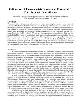
Figure
1.
Calibrating
the
alcohol
thermometer
(white)
to
the
ASTM
mercury
thermometer
(yellow)
in
a
dewar
filled
with
ice
water.
In
the
background,
the
Davis
weather
station
thermometer
probe
is
concealed
inside
of
the
louver-­‐‑style
shelter.

10. Rux,
V.
|
10
Figure
2.
Adding
warm
water
to
the
dewar
while
calibrating
the
Davis
weather
thermometer
probe
to
the
alcohol
thermometer.
The
temperature
for
the
Davis
is
read
using
the
Davis
Weather
Monitor.
Figure
3.
Allowing
the
thermometers
to
come
to
equilibrium.
The
Davis
monitor
is
more
visible.
Also,
in
the
background,
the
Variac
dial
is
visible.
That
device
controls
the
wind
velocity
through
the
wind
tunnel.

11. Rux,
V.
|
11
Figure
4.
The
bead
thermistor
being
calibrated
to
the
alcohol
thermometer
and
a
voltmeter
reads
the
resistance
from
the
thermistor.
Conversion
is
0.01
Volts
=
1°C.
Figure
5.
Wind
tunnel
apparatus
with
the
alcohol
thermometer
and
the
Davis
thermometer
sitting
in
a
dewar
of
hot
water
before
calculating
the
time
response
for
the
thermometers
to
reach
an
equilibrium
temperature.

12. Rux,
V.
|
12
Figure
6.
(above).
The
ASTM
thermometer
calibration
to
the
NIST
standard.
Each
value
was
tested
was
from
the
calibration
certificate.
Figure
7.
(below).
The
alcohol
thermometer
calibration
to
the
ASTM
thermometer.
Each
data
point
represents
a
best
estimate
average
of
each
trial.
The
reference
thermometer
on
the
y-­‐‑axis,
the
observed
thermometer
on
the
x-­‐‑axis.

13. Rux,
V.
|
13
Figure
8.
(above).
Davis
thermometer
calibration
to
the
Alcohol
thermometer.
Each
data
point
represents
a
best
estimate
average
of
each
trial.
The
reference
thermometer
on
the
y-­‐‑
axis,
the
observed
thermometer
on
the
x-­‐‑axis.
Figure
9.
(below).
Bead
thermistor
calibration
to
the
NIST
standard.
Each
data
point
represents
a
best
estimate
average
of
each
trial.
The
reference
thermometer
on
the
y-­‐‑axis,
the
observed
thermometer
on
the
x-­‐‑axis.

14. Rux,
V.
|
14
Thermometer Slope Slope error Intercept (°C) Intercept error (°C) R2
ASTM mercury 1.00 0.00 0.01 0.01 1.00
Alcohol 0.97 0.00 0.04 0.04 0.99
Davis 1.03 0.01 -0.01 0.08 0.99
Bead Thermistor 1.05 0.01 -0.52 0.13 0.99
Thermometer Total Error (°C) Rank
ASTM to NIST 0.02 1
Alcohol to NIST 0.33 2
Davis to NIST 0.54 4
Bead Thermistor to NIST 0.49 3
Table
1.
The
linear
regression
output
for
each
thermometer
based
on
the
calibration
data
in
figures
6-­‐‑9.
R2
shows
how
well
our
data
was
represented
by
the
linear
fit
relationship.
Table
2.
The
total
error
for
each
thermometer
based
on
the
calibration
data
in
figures
6-­‐‑9.
Each
thermometer
calibration
was
ranked
from
the
least
amount
of
error
to
the
largest
error
respective
to
the
NIST
standard.

15. Rux,
V.
|
15
Figure
10.
(above).
The
exponential
decay
of
five
trials
using
the
alcohol
thermometer
subjected
to
ventilation
in
seconds.
Figure
11.
(below).
The
exponential
decay
of
five
trials
using
the
Davis
temperature
probe
subjected
to
ventilation
in
seconds.

16. Rux,
V.
|
16
Figure
12.
The
time
constant
of
five
trials
using
the
alcohol
thermometer
and
the
Davis
temperature
probe
subjected
to
ventilation
in
seconds.
Linear
regression
fitting
was
generated
to
see
how
linear
the
relationship
was
for
the
time
response
on
wind
speed.
The
time
constant
decreases
as
the
wind
speed
increases.
Changes
in
response
are
notable
around
1
m/s
when
the
response
sensitivity
switches
from
the
Davis
being
more
responsive
than
the
alcohol
thermometer
to
the
alcohol
thermometer
being
more
responsive
at
higher
ventilation.

17. Rux,
V.
|
17
Thermometer Slope Slope error Intercept (s) Intercept
error (s)
R2
Alcohol -55.91 5.38 142.05 9.94 0.97
Davis -26.62 6.35 116.35 11.91 0.85
Thermometer Wind Speed
(m/s)
Time constant, τ
(s)
Error
𝝈 𝝉 (s) 1/e (s-1
) Rank
Alcohol 0 145.22 41.52 -0.01 1
1.85 25.26 5.35 -0.04 3
1.97 29.79 2.43 -0.03 2
2.21 21.06 2.17 -0.05 4
2.36 20.06 2.19 -0.05 5
Davis 0 112.82 33.00 -0.01 1
1.85 75.44 231.24 -0.01 3
1.97 77.58 227.09 -0.01 2
2.18 51.31 76.13 -0.02 4
2.36 42.23 53.62 -0.02 5
Table
3.
The
linear
regression
output
for
each
the
time
constant
in
figure
12.
R2
shows
how
well
our
data
was
represented
by
the
linear
fit
relationship.
The
alcohol
had
a
better
linear
relationship
compared
to
the
Davis
thermometer.
Table
4.
The
ranking
from
largest
to
smallest
of
the
1/e
decay
for
each
thermometer.
It
was
not
quite
perfectly
linear
with
speed
but
it
was
very
close
to
linear.
The
time
constant
for
the
alcohol
thermometer
shows
how
at
little
to
no
wind
velocities,
the
response
time
is
large
but
at
higher
velocities,
the
response
time
is
quite
low
compared
to
the
Davis
thermometer.

18. Rux,
V.
|
18
SYMBOLS MEANING
𝑹 𝟐 a coefficient of determination: how well the regression line represents the real data
𝑵 number of observations in a sample
𝒊 index or iteration
𝒎 the slope generated from the linear regression
𝒄 the intercept generated from the linear regression
𝑻𝒊,𝒐𝒃𝒔 observation temperature at the iteration
𝑻 𝒇𝒊𝒕 the temperature output given by the linear regression
𝑺 𝒐𝒃𝒔
𝟐 the variance between the observed temperature and the linear regression
𝑺 𝒓𝒆𝒇
𝟐 the variance of the the reference temperature given the linear regression and the
variance of the observed thermometer
𝑻 𝒐𝒃𝒔 the mean temperature of the observed thermometer for all trials to one reference
𝝈 𝒎 standard deviation of the slope from the linear regression
𝝈 𝒄 standard deviation of the intercept from the linear regression
𝝉 time constant
𝒕 time seconds
∆𝑻 change in the temperature reading to the ambient temperature
Tambient ambient temperature
∆𝑻 𝒎𝒂𝒙 change in the initial temperature to the ambient temperature
°C temperature in degrees Celsius
m meters
s seconds
Table
5.
Symbols
from
mathematical
formulas
and
figures.