Stochastic life cycle costing

APPLICATION NOTE
STOCHASTIC LIFE CYCLE COSTING DEALING WITH
UNCERTAINTY AND VARIABILITY
Forte
March 2017
ECI Publication No Cu0166
Available from www.leonardo-energy.org

Publication No Cu0166
Issue Date: March 2017
Page i
Document Issue Control Sheet
Document Title: Application Note – Advanced LCC
Publication No: Cu0166
Issue: 02
Release: Public
Content provider(s) Joris Debonnet
Author(s): Forte (Joris Debonnet and Diedert Debusscher
Editorial and language review Bruno De Wachter (editorial), Noel Montrucchio (English language)
Content review: Ecofys (Edwin Haesen)
Document History
Issue Date Purpose
1 July 2012 Initial publication in the framework of the Good Practice Guide
2 March
2017
New version after review (and updates ModelRisk software)
3
Disclaimer
While this publication has been prepared with care, European Copper Institute and other contributors provide
no warranty with regards to the content and shall not be liable for any direct, incidental or consequential
damages that may result from the use of the information or the data contained.
Copyright© European Copper Institute.
Reproduction is authorized providing the material is unabridged and the source is acknowledged.

Issue Date: March 2017
Page ii
CONTENTS
SUMMARY ........................................................................................................................................................ 1
INTRODUCTION .................................................................................................................................................. 2
STEP 1 – MODEL UNCERTAIN AND VARIABLE INPUTS AS DISTRIBUTIONS .................................................................... 5
CRASH COURSE IN STATISTICS.......................................................................................................................................5
USEFUL DISTRIBUTIONS IN AN LCC CONTEXT .................................................................................................................7
CHOOSING THE RIGHT DISTRIBUTION FOR YOUR COST PARAMETERS ..................................................................................8
STEP 2 – RUN A MONTE CARLO SIMULATION ....................................................................................................... 11
STEP 3 – ANALYZE THE MONTE CARLO SIMULATION RESULTS................................................................................. 13
STEP 4 – PERFORM A SENSITIVITY ANALYSIS ........................................................................................................ 16
STEP 5 – MAKE WELL-FOUNDED DECISIONS ........................................................................................................ 21

Issue Date: April 2017
Page 1
SUMMARY
Life Cycle Costing (LCC) analysis helps you compare several investment opportunities based on the costs and
revenues each investment generates over several years. You learned how to perform a simple LCC in the first
Application Note.
Basic LCC is a good method for making informed decisions, but the outcome of such an analysis depends
heavily on the quality of the input data and the assumptions you make. Energy prices, maintenance expenses,
availability and discount rates are just some of the parameters you need to estimate. But it doesn’t stop there.
You also need to able to defend your estimates. After all, each parameter can have a huge impact on your final
decision. A critical audience, such as your management or funders, will undoubtedly test the robustness of
your decision.
You can strengthen your case by including a sensitivity and risk analysis – in other words, perform a stochastic
LCC analysis. It doesn’t necessarily require more or better information than a basic LCC analysis, but it does
allow you to deal more effectively with the limited information at your disposal. A sensitivity analysis shows
you how robust your decision is: in other words, would your choice between several investment opportunities
change if any of the input parameters changed? A risk analysis shows you which risks you could manage to
safeguard the profitability of your project.
This Application Note will teach you the basics of Monte Carlo Simulation, a powerful method that allows you
to deal with risks and uncertainty by building and running a stochastic LCC model. Each step in the 5-step
procedure is illustrated with a running example, which you can check yourself in MS Excel, using the free trial
version of a software add-in.

Page 2
INTRODUCTION
After reading this chapter you will know the difference between uncertainty and variability and will understand
how both phenomena can lead to risk. It is essential to take them into account during an LCC analysis in
general and during the financial evaluation of Energy Efficiency Projects in particular.
As you will have noticed in the example at the end of the first Application Note on LCC, Leonard’s final decision
between his three options (base case, alternative A or alternative B) depends heavily on his assumptions and
the quality of his input data. Energy prices, maintenance expenses, availability and discount rates; these are
just some of the parameters Leonard used to derive estimates that seem reasonable and defensible, but not
quite beyond doubt. Can you imagine him presenting his results to the board of directors? Surely, a critical
audience would try to test the robustness of his decision. Would his advice to invest €35,000 in option B still
stand if energy prices plummeted, if the downtime was substantially underestimated or if his CFO was not
convinced of the discount rate? If Leonard wants to give a satisfactory answer to these questions, he should
include a sensitivity and risk analysis in his report. By taking the uncertainty and variability into account during
his LCC analysis, Leonard would make his case stronger and the risks in his decision would become
manageable.
Before we provide you with a practical approach for this, let’s first clarify what we mean by these important
terms uncertainty, variability and risk:
 Uncertainty refers to a condition of the observer. Due to a lack of precise knowledge, he or she does not
know which exact value to choose for a certain parameter. For example, you probably do not know the
exact average height of a Belgian man. You might guess it is 1.75 m, but you would probably acknowledge
that this estimate is somewhat uncertain. This uncertainty can be reduced by collecting more and better
information. If you look on, say, Wikipedia, you will find the average height of Belgian men was 1.795 m
in 2005; your uncertainty is reduced. That is the essential characteristic of uncertainty: it can be
diminished through further study.
 Variability refers to inherent variations that are present in some systems, which will always exist,
regardless of how much information is collected. Variability expresses the random differences in the
nature of the object of study. If you have to guess the height of a randomly chosen Belgian man, you
could use the average of 1.795 m as your best estimate, but the actual height may be different.
 Risk is a word that is associated with a potential adverse outcome: e.g. a possibility of financial loss or
injury. Both variability and uncertainty can lead to risk. If you bet €100 on guessing the exact average
height of Belgian men without access to the correct information, your uncertainty puts you at risk. The
risk is even higher if you bet on guessing the height of a randomly chosen individual; but then it is mainly
the variability that puts you at risk.
In Energy Efficiency projects, the following typical uncertain and/or variable factors can be encountered:
 future energy prices
 energy consumption rates
 cost of capital and inflation rates
 number of operational hours and loading factors
 failure rates of equipment and the time and resources necessary to remediate them
 consequences of downtime (e.g. penalty rates)
 …
In order to deal with these factors, you should carefully assess their influence on the LCC and the profitability
of your alternatives. This can be done using a stochastic approach to LCC, which essentially does not treat cost
factors as a single number (e.g. the maintenance expense of a pump will be exactly €500 per year) but rather

Page 3
models them as a statistical distribution (e.g. the maintenance expense of a pump will be between €300 and
€800 per year, with each value in this range having an equal probability of occurring in a given year). A
stochastic LCC model can be used to perform a sensitivity analysis, which allows you to see how your choice
between several investment opportunities can change when input parameters change. This helps you to find
out how robust your decision is (does it hold if certain inputs vary?) and which risks you should be able to
manage in order to safeguard the profitability of your project.
In this Application Note, we will teach you the basics of Monte Carlo Simulation, a powerful method that
allows you to build and run a stochastic LCC model. A few decades ago, the application of Monte Carlo
Simulation (MCS) was left to specialized research laboratories, but now, due to the revolutionary increase in
computation power of widely available personal computers, MCS is within everyone’s reach. Since practical
experience of an MCS model will teach you more than a thousand pages of theory, we ask you to try to solve
the exercise presented in the text boxes. You will need MS Excel on your PC and you will have to install the
free trial version of the software add-in ‘ModelRisk’, a program that runs inside MS Excel
1
.
The structure of this Application Note reflects the five steps of a stochastic LCC analysis procedure:
1. Model uncertain and variable inputs as distributions
2. Run a Monte Carlo Simulation (MCS)
3. Analyze the MCS results
4. Perform a Sensitivity Analysis
5. Make well-founded decisions
These steps assume that you have carried out all the work of the first Application Note, such as defining the
scope of your model and building a Cost Breakdown Structure.
Before we start with the first of these five steps, we want to refute an often cited objection to stochastic LCC
analysis, namely that it is impossible because there is not enough ‘statistical’ information about cost inputs.
This must be the biggest misconception about stochastic LCC because the techniques presented here do not
require more or better information than basic LCC analysis, but actually allow you to deal more effectively with
the limited information at your disposal.
1
You can download the ModelRisk trial at http://www.vosesoftware.com/products/modelrisk/, where you’ll
also find an installation guide. Registration is required to receive a user ID.

Page 4
INTRODUCTION TO THE EXAMPLE: Leonard is still concerned with the decision problem introduced in the
first Application Note. Since he has to present his findings during the board meeting, he wants to strengthen
his case by looking at how robust his decision for alternative B is. Leonard wants to identify the uncertainties
and variabilities that pose the biggest risk for the profitability of alternatives A and B in comparison to the
base case. Therefore, he consults all experts again and reinterprets all data at his disposal. The results of his
efforts are presented in the table below. For each of the different uncertain or variable cost parameters, the
minimum, maximum and – if known – most likely value is presented.
BASE CASE ALTERNATIVE A ALTERNATIVE B
Discount rate % minimum 9.0% 9.0% 9.0%
% maximum 12.0% 12.0% 12.0%
Annual maintenance cost €/year minimum 4,700 4,800 2,500
€/year most likely 4,800 5,200 4,000
€/year maximum 4,900 5,300 5,500
Maintenance cost increase
after 5 years %
in 30% of the
cases 70.00% 20.00% 30.00%
%
in 70% of the
cases 50.00% 50.00% 0.00%
Energy Consumption kWh/year minimum 94,000 72,000 48,000
kWh/year most likely 98,000 75,000 61,000
kWh/year maximum 105,000 78,000 78,000
Energy price €/kWh minimum 0.12 0.12 0.12
€/kWh maximum 0.18 0.18 0.18
Availability % minimum 95.70% 99.10% 97.80%
% most likely 98.70% 99.50% 99.70%
% maximum 99.50% 99.70% 99.93%
Penalty cost €/hour minimum 45 45 45
€/hour maximum 55 55 55
TABLE 1: CHARACTERISTICS OF THE THREE ALTERNATIVES.
Which decision should Leonard take? Should he keep the old system running or replace it with alternative A or B?
RECAP – THE CASE FOR STOCHASTIC LCC ANALYSIS
A stochastic LCC analysis allows you to identify which of the numerous variabilities and uncertainties inherent
in your LCC analysis pose the largest risk. It highlights which risks you should be able to manage in order to
safeguard the profitability of your energy efficiency projects.

Page 5
STEP 1 – MODEL UNCERTAIN AND VARIABLE INPUTS AS DISTRIBUTIONS
After reading this chapter you will know how to model uncertain and variable cost parameters by using
probability functions. You will be acquainted with some of the most useful functions in the context of Energy
Efficiency Projects.
When you want to turn your basic LCC model from the previous Application Note into a stochastic LCC model,
the first thing that you should do is model your uncertain and/or variable input parameters as statistical
distributions.
CRASH COURSE IN STATISTICS
In statistics, we are dealing with random processes, random variables, distribution functions and statistical
measures such as mean, mode, standard deviation and percentiles. We will briefly refresh your knowledge of
these concepts, assuming they already sound familiar to you. If this is not the case, refer to any basic statistical
textbook for further explanation.
 A random variable is a variable that takes values according to some random process. An example of a
simple random process is the tossing of a coin, resulting in either heads or tails. The random variable
defined in relation to this random process is: A(C) = 0 if C = heads and A(C) = 1 if C = tails. Since A(C) can
only take a limited number of values, it is a discrete random variable. A continuous random variable, on
the other hand, can take a whole range of values in a certain interval, e.g. any real number between 3
and 4.
 A statistical distribution function is a function that describes the probability of a random variable taking
certain values. Let’s first focus on two types of distribution functions commonly used to characterize a
discrete random variable: the probability mass function (pmf) and the cumulative distribution function
(cdf). The pmf assigns to each possible outcome the probability that the random variable is equal to a
certain value, while the cdf describes the probability that it is smaller than or equal to this value. In
practice, all probabilities in the pmf should add up to 1 and the cdf always starts at 0 and ends at 1.
Consider as an example a discrete random process that has a 25% probability of generating the value 1,
50% of 2, 20% of 3 and 5% of 4. Its pmf and cdf are presented in Figure 1.
Figure 1 – Probability mass function (pmf) and cumulative distribution function (cdf) for a discrete random
variable.

Page 6
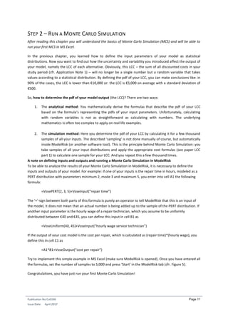
 Continuous random variables can be described by their probability density function (pdf) and their
cumulative distribution function (cdf). Let’s explain them with the following example: the random
variable B(P) takes as its value the height of a randomly chosen male adult person P. Since in principle it
can take any value between 0.50 m and 2.50 m, it is a continuous random variable. B(P) is most likely to
be between 1.50 m and 2.00 m, and only in rare cases below 1.50 m or above 2.00 m, so its probability in
the interval [1.50 m, 2.00 m] will be higher than outside of this interval. This can be expressed by the pdf
of B(P), depicted on the left side of Figure 2. You will probably recognize the bell shape of the Normal
distribution, which is the most prominent distribution found throughout nature. The pdf should be
interpreted as follows: the probability of B(P) taking a value between 1.84 m and 1.88 m is given by the
area shaded in dark gray in the picture. On the right side of Figure 2 we depict its cdf. This is just one
possible conclusion that you can derive by looking to this cdf: the probability that the height of a man is
smaller than or equal to 1.92 m is about 96%.
Figure 2 – Probability density function (pdf) and cumulative distribution function (cdf) for a Normal distribution.
Apart from distribution functions, these are some important statistical measures commonly used to
characterize random variables (indicated on an example pdf in Figure 3):
Figure 3 – Statistical measures indicated on an example pdf.
 The mean μ tells you which value the random variable will take on average. The calculation of this
average is ‘probability weighted’, taking into account not only the range of possible values of a random
variable, but also how likely the values in this range are occurring.
 The mode α is the single most likely value for a random variable. It is the value for which the pdf reaches
it maximum. The mode is not necessarily the same as the mean, although in the example of Figure 2 it is.

Page 7
 The standard deviation σ is the absolute value of the mean deviation of all data points to the mean
value. For a Normal distribution, the probability that a random variable will take a value in the interval [μ
– σ; μ + σ] is 68% and the probability that it will be in the interval [μ – 2σ; μ + 2σ] is 95%.
 The x-th percentile px gives you the value for which the probability that the random variable is smaller
than px is x%. For example, the 90
th
percentile p90 tells you the value for which there is a 90% probability
that your random variable is smaller than p90. The 10
th
percentile p10 tells you the value for which there
is a 10% probability that your random variable is smaller than p10. The 50
th
percentile p50 is also known
as the median.
USEFUL DISTRIBUTIONS IN AN LCC CONTEXT
There are many types of statistical distributions, continuous as well as discrete. After installing ModelRisk,
open MS Excel open the MODELRISK tab, and click on the icon ‘Select Distribution’. A pop-up window shows
you the wide variety of continuous and discrete distributions available within this software package. Within a
typical LCC analysis for the sort of cost parameters that we are facing, however, we can limit ourselves to four
common types of continuous distributions, namely the Uniform, Triangular, PERT and Normal distribution,
and one type of discrete distribution.
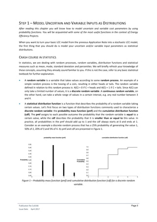
 A Uniform distribution is characterized by the minimum m and maximum M. It assigns equal probability
to all values between m and M. As you can see on the left side of Figure 4, its pdf is a straight line
between m and M and zero outside of this interval. It is defined in ModelRisk as VoseUniform(m, M).
 The Triangular distribution is characterized by the minimum m, mode α and maximum M. Its pdf has the
form of a triangle, as you can see in the second graph from the left in Figure 4. The values closer to the
mode are more likely to occur than the value near minimum or maximum. It is defined in ModelRisk as
VoseTriangle(m, α, M).
 The PERT distribution is characterized by the minimum m, mode α and maximum M. It is actually a
special version of the Beta-distribution. Similar to the Triangular distribution, it assigns a higher
probability to values near the mode, and a lesser one to values near minimum or maximum, as you can
see on the third graph of Figure 4. In comparison to the Triangular distribution, values are even more
likely to be generated near the mode and less likely near the extremes (m and M). It is defined in
ModelRisk as VosePERT(m, α, M).
 The already mentioned Normal distribution is characterized by the mean μ and standard deviation σ and
depicted on the right side of Figure 4. It has no minimum or maximum value. It is defined in ModelRisk as
VoseNormal(μ, σ).
Figure 4 – Probability density functions (pdfs) of a Uniform, Triangular, PERT and Normal distribution.

Page 8
A wide variety of discrete distributions types exist, but in the context of this Application Note, one will suffice,
namely the flexible ‘Discrete distribution’:
 The Discrete distribution is characterized by a number of values and their corresponding probabilities. It
is defined in ModelRisk as VoseDiscrete({Value1, Value2,…,ValueK}, {Prob1, Prob2,…, ProbK}). For the
example mentioned in Section 1.1, for which the pmf is shown in Figure 1, the implementation in
ModelRisk would be as follows: VoseDiscrete({1, 2, 3, 4}, {25, 50, 20, 5}). The following implementation is
completely equivalent to this one: VoseDiscrete({1, 2, 3, 4}, {0.25, 0.5, 0.2, 0.05}), so you can choose
either one.
A note on inserting distributions in ModelRisk
ModelRisk allows you to directly insert a complete distribution into one single cell in MS Excel. If you want to
enter a Normal distribution with mean 100 and standard deviation 10 into a cell, do this by typing
=VoseNormal(100, 10) into the cell and pressing the enter button. You will see that a value generated by this
distribution is displayed in the cell. This value is sampled by the ModelRisk-function from the distribution you
defined. Now, each time you press ‘F9’, another value is sampled. Now it’s your turn: try to implement
examples of all five provided distributions and press F9 a few times. In Chapter 2, we will teach you how to run
a simulation, which is actually like pressing F9 a few thousand times and thus sampling values from the
inserted distributions. But let’s first give the practical advice we had promised you on choosing a suitable
distribution for your specific cost parameters.
CHOOSING THE RIGHT DISTRIBUTION FOR YOUR COST PARAMETERS
By now, you have learned the five most common distributions that can be applied to model the uncertainty
and/or variability present in the input parameters of your LCC model. This leaves you with the question: which
one should I choose under which circumstances? Here are some guidelines to help you choose:
 The general principle is that you should choose the type of distribution that is the best representation of
the variability and/or uncertainty present in your cost parameter. If, for example, a parameter can only
take three values, the most logical choice is to select a discrete distribution.
 In principle, all statistical textbooks advise you to separate uncertainty from variability in your stochastic
LCC model by making two different distributions. In doing so, you can clarify whether it makes sense to
acquire more information. But often it is difficult to determine where uncertainty ends and variability
begins. Consider, for example, the evolution of energy prices: are they uncertain or variable? In fact, they
are both; well-informed analysts probably know the main factors that drive energy prices up or down,
and by acquiring their knowledge, your uncertainty could be reduced. But due to the complex manner in
which energy prices are determined by numerous unpredictable factors, such as climate conditions and
geopolitical events, there will always remain a significant amount of variability. So, in practice, it is not
always feasible to separate both phenomena. That’s why this advice should be followed pragmatically
rather than dogmatically. Wherever possible, don’t model uncertainty and variability with one single
distribution.
 The Normal distribution is recommended for modeling parameters that are calculated as the sum of a
large set of random variables, on condition that none of these variables are dominant. If, for example,
you want to model a measurement error, and this error is derived as the sum of 50 small errors which
occur due to different reasons, it can best be modeled by a Normal distribution. But beware that the
Normal distribution can attain in principle any value between -∞ and +∞, while the Uniform, Triangular
and PERT distribution have a minimum and maximum value.
 The Uniform distribution is recommended when you can assign to a particular cost parameter a range of
possible values between a minimum and a maximum, but you don’t really have an idea which value in

Page 9
this range is the most likely. In other words, if you are really uncertain about the distribution of the
parameter between minimum and maximum, choose the Uniform distribution, since it assigns equal
probability to each value within the range. On the other hand, it is often less suitable for modeling expert
opinion because experts do usually have an idea which values are most likely to occur.
 The PERT and Triangular distributions are particularly useful for modeling expert opinion. Experts can
usually give you estimates about a parameter by stating its minimum, maximum and mode, and do have
an intuitive feeling that the parameter will probably be nearer to the mode and will less likely be near the
extremes. As you see in Figure 4, in the Triangular distribution, the probability decreases linearly from the
mode to the extremes, while in the PERT distribution the decrease in probability is more gradual in the
beginning and more rapid near the extremes. That’s why it is said that the PERT distribution assigns less
‘weight’ to the extremes, which makes it a popular choice for modeling expert estimates. But, in practice,
the difference between the PERT and Triangular distribution is minor.
In this Application Note, we’ve discussed the five types of distributions most common in the context of Energy
Efficiency Projects. For the sake of completeness, we mention the name and main practical applicability of
other distributions you might encounter:
 The lifetime of a component or a product is often modeled as an Exponential distribution (if the
probability of failure is independent of the component age) or as a Weibull distribution (if the failure
probability increases or decreases with component age).
 If the probability that a certain event (e.g. a technical failure) occurs is the same at each moment, the
Poisson distribution is the discrete distribution that represents the number of events within a certain
timeframe (e.g. the number of light bulbs that need to be replaced within a period of one year in a
building). The Gamma distribution is a continuous distribution that represents the time that passes until
N events occur (e.g. the elapsed time until 100 light bulbs need to be replaced).
 If an expert has detailed information on the distribution of a cost parameter, the Modified PERT or
Relative distribution might come in handy, since they are very flexible to model a ‘custom-made’ pdf.
 Analogous to the Normal distribution, the Lognormal distribution is often used to describe parameters
that are derived as the product of a large set of random variables.

Page 10
EXAMPLE: Leonard has chosen distributions for his different cost parameters. You can see his reasoning in
the table below.
Cost Parameter … … is modeled as a … … because …
Energy price
Uniform Distribution
between 0.12 and
0.18 €/kWh
…Leonard chooses to simplify his study and includes the average
energy price over the total study period as a uniformly distributed
parameter. He chooses its range as follows: as a minimal value he
selects the current end-user energy price for industrial customers
in Belgium as published on www.energy.eu (0.12 €/kWh) and as a
maximum he chooses a 50% increase of the average relative to
the current price level (0.18 €/kWh) over the total study period.
Alternatively, he could rely on specialized models for energy price
forecasting (e.g. time series models), but Leonard does not wish to
complicate his study more than necessary and prefers the Uniform
Distribution; it has the advantage that a straightforward sensitivity
analysis can be carried out (cfr. Chapter 4).
Discount Rate
between 9 and 12%
…the CFO of his company provided a minimum and maximum for
the company’s WACC, but could not say which value is most likely
within this range.
Penalty Cost
between 45 and 55
€/hour
…the cost of putting a backup pump in operation is estimated
within this range and Leonard has no information which value is
most probable.
Maintenance Cost
Increase
Discrete Distribution
… there is a 30% probability that due to changing safety
regulations the cost of specific maintenance tasks will increase for
the base case and alternative B, but will decrease for alternative A.
Energy Consumption
Triangular
Distribution
… the specialist he interviewed said he expects a triangular
distribution to be the best representation of the uncertainty of
this parameter. The simplification is made here to express the
yearly energy consumption as one single parameter. This
parameter can also be decomposed into the product of the yearly
operational hours and the electrical input power of each pump (in
kW), a parameter which in its turn depends on the pumps
efficiency and other application parameters such as the flow rate
and the fluid density, but Leonard chooses to simplify his model by
limiting the total number of parameters. If the sensitivity analysis
would indicate that the uncertainty of this parameter is important
for the uncertainty of the LCC, he will decompose it further.
Annual Maintenance
Cost, Availability
PERT Distribution … these parameters are expert estimates and the values near the
extremes are less likely to occur.
RECAP – STEP 1: MODEL UNCERTAIN AND VARIABLE INPUTS AS DISTRIBUTIONS
In most cases, LCC input parameters can be modeled with one of these distribution types: Uniform,
Triangular, PERT, Normal or Discrete distribution. For each of your input parameters, you should choose
the distribution type that is most suitable for representing the underlying variability or uncertainty.

Page 11
STEP 2 – RUN A MONTE CARLO SIMULATION
After reading this chapter you will understand the basics of Monte Carlo Simulation (MCS) and will be able to
run your first MCS in MS Excel.
In the previous chapter, you learned how to define the input parameters of your model as statistical
distributions. Now you want to find out how the uncertainty and variability you introduced affect the output of
your model, namely the LCC of each alternative. Obviously, this LCC – the sum of all discounted costs in your
study period (cfr. Application Note 1) – will no longer be a single number but a random variable that takes
values according to a statistical distribution. By defining the pdf of your LCC, you can make conclusions like: in
90% of the cases, the LCC is lower than €10,000 or: the LCC is €5,000 on average with a standard deviation of
€500.
So, how to determine the pdf of your model output (the LCC)? There are two ways:
1. The analytical method: You mathematically derive the formulas that describe the pdf of your LCC
based on the formula’s representing the pdfs of your input parameters. Unfortunately, calculating
with random variables is not as straightforward as calculating with numbers. The underlying
mathematics is often too complex to apply on real life examples.
2. The simulation method: Here you determine the pdf of your LCC by calculating it for a few thousand
samples of all your inputs. The described ‘sampling’ is not done manually of course, but automatically
inside ModelRisk (or another software tool). This is the principle behind Monte Carlo Simulation: you
take samples of all your input distributions and apply the appropriate cost formulas (see paper LCC
part 1) to calculate one sample for your LCC. And you repeat this a few thousand times.
A note on defining inputs and outputs and running a Monte Carlo Simulation in ModelRisk
To be able to analyze the results of your Monte Carlo Simulation in ModelRisk, it is necessary to define the
inputs and outputs of your model. For example: if one of your inputs is the repair time in hours, modeled as a
PERT distribution with parameters minimum 2, mode 3 and maximum 5, you enter into cell A1 the following
formula:
=VosePERT(2, 3, 5)+VoseInput(“repair time”)
The ‘+’-sign between both parts of this formula is purely an operator to tell ModelRisk that this is an input of
the model, it does not mean that an actual number is being added up to the sample of the PERT distribution. If
another input parameter is the hourly wage of a repair technician, which you assume to be uniformly
distributed between €40 and €45, you can define this input in cell B1 as
=VoseUniform(40, 45)+VoseInput(“hourly wage service technician”)
If the output of your cost model is the cost per repair, which is calculated as (repair time)*(hourly wage), you
define this in cell C1 as
=A1*B1+VoseOutput(“cost per repair”)
Try to implement this simple example in MS Excel (make sure ModelRisk is opened). Once you have entered all
the formulas, set the number of samples to 5,000 and press ‘Start’ in the ModelRisk tab (cfr. Figure 5).
Congratulations, you have just run your first Monte Carlo Simulation!

Page 12
Figure 5 – Setting the number of samples and pressing the start button in the ModelRisk tab in MS Excel.
EXAMPLE: Open the MS Excel file ‘LCC_MCS.xls’ that Leonard constructed to calculate the LCC of his three
different options. In this file, the input values of Leonard’s data gathering activities are in the yellow cells,
while the distributions he based upon these are in the orange cells. Two parameters are missing in this
model, which you’ll need to complete:
 the Uniform Distribution of the energy price between 0.12 and 0.18 €/kWh. In addition to entering the
distribution function, this cell should also be defined as an input “Energy price” in cell D47.
 the PERT Distribution of the availability of the three options. They should all be defined as inputs with
parameters given in row 48, 49 and 50 into cells D51, E51 and F51 respectively, and defined as inputs
“availability base case”, “availability ALT A” and “availability ALT B”.
Once you have performed this ‘finishing touch’ to the model, set the number of samples to 5,000 and run the
simulation by pressing ‘Start’.
RECAP – STEP 2: RUN A MONTE CARLO SIMULATION
After defining all the inputs and outputs of your Monte Carlo Simulation model, set the number of
simulations to 5,000 and run it.

Page 13
STEP 3 – ANALYZE THE MONTE CARLO SIMULATION RESULTS
After reading this chapter you will be able to analyze the output distributions of an MCS model.
Now you know how to run a Monte Carlo Simulation, you’ll need to learn how to analyze its results. For this,
you need the ‘Results’ window of ModelRisk, which opens automatically after each simulation. You can also
open it manually by pressing the ‘Results’ button in the ModelRisk tab (cfr. Figure 5, next to ‘Start’). In this
chapter, we focus completely on the running example.
EXAMPLE: In the results window on the left side, you can select the inputs and outputs you want to examine
by checking a box next to their name. The icons in the Insert tab allow you to choose different display types.
We will discuss three of them: the histogram, the cumulative ascending plot and the ‘Stats’.
Select the Histogram (Figure 6, Nr. 1) and then check the boxes for outputs ‘LCC ALT A’, ‘LCC ALT B’ and ‘LCC
base case’. This histogram is an estimate of the pdf of these random variables, based on the 5,000 samples
that were calculated during the simulation. The outputs of this simulation are grouped into classes (i.e. values
that fall within a certain interval) and the height of the bar is the probability that the output falls within this
interval. Apart from this standard visualization, the chart mode can also be changed to Line in the Histogram
Options tab (Figure 7, Nr. 1). Do this for each of the three distributions. Also put Show Sliders off (Figure 7,
Nr. 2) and the Show Legends on (Figure 7, Nr. 3).
Now that you see how the LCC for each of the three considered scenarios is distributed, you should be able to
derive the graph depicted in Figure 8. What conclusions can you draw from this visualization? Try to find
them yourself before reading on.
Conclusions based on the pdf visualization:
1. In most cases, LCCbase case seems to be significantly larger than LCCA and LCCB: notice how the pdf of
LCCbase case is generally positioned more to the right, with its minimum value around €110,000 and its
maximum around €220,000. The difference between LCCA and LCCB is less. This graph indicates that,
in any case, it makes sense to choose alternative A or B over the base case.
2. The spread of the distribution indicates how variable and uncertain each LCC is. Notice how large the
spread of the base case is, compared to alternative A or B. The spread of LCCA is smaller than the
spread of LCCB, even though LCCA seems to be a bit larger on average.
Now switch to the cumulative ascending plot (by clicking icon Nr. 2 of Figure 6) and you will see the cdfs of
the three LCC options. Your previous conclusions are confirmed: look at the position of the cdfs on the
horizontal axis. By moving the cursor over the graphs, you’ll get a hint of the X and Y values (the LCC and
corresponding cumulative percentage). Try to answer these questions (Note in advance: since each
simulation will lead to a different set of 5,000 samples, the numerical values you obtain will probably be
somewhat different but close to the numbers below):
1. What is the median for each of the three distributions? (Answer: around €156,700 for LCCbase case,
€128,800 for LCCA, and €124,300 for LCCB)
2. What is P90 for each of the distributions? (Answer: P90 is near to €184,300 for LCCbase case, €140,700 for
LCCA and €142,400 for LCCB)

Page 14
Figure 6 – Display types in the Results window of ModelRisk that are discussed in this Application Note.
Figure 7 – Histogram Options: chart mode Bars or Line (1), slider on/off (2), legends on/off (3).
You can consult the actual values for the different statistical measures (Cfr. Section 1.1) by clicking the ‘Stats’
icon (Nr. 3 in Figure 6). Check the mean, the standard deviation and the different percentiles for each
distribution. If the mean LCC would be your sole decision criterion, you would choose alternative B over
alternative A. But the spread of LCCB is wider than the spread of LCCA: the standard deviation of LCCB is
almost €3,700 larger than that of LCCA.
Now try to analyze the histogram, cumulative ascending plot and statistics for the other two outputs that
were defined: ‘NPV A’ and ‘NPV B’. These are the Net Present Value of all the cost savings over the base case
realized by alternative A or B respectively. The key question is: in percentage terms, how many of the cases
will have a loss over the base case for option A and B? The cumulative ascending plot can tell you this.
(Answer: in about 1.5% of the cases for alternative A and in almost 4.5% of the cases for alternative B)
At this point, all elements are present to make your final decision. However, since drawing conclusions from a
statistical analysis is an art in itself, we devote a complete chapter to it (Chapter 5). But first we’ll teach you
how to perform a sensitivity analysis.
1 2 54 3
1 2 3

Page 15
Figure 8 – Histogram plot for the three alternatives.
RECAP – STEP 3: ANALYZE THE OUTPUT DISTRIBUTION OF YOUR MONTE CARLO SIMULATION
Interpret the results of your MCS model by analyzing its pdf, cdf and statistics.

Page 16
STEP 4 – PERFORM A SENSITIVITY ANALYSIS
After reading this chapter you will understand what sensitivity analysis is, and you will be able to identify the
input parameters that contribute most to the total variation of your MCS model’s output. You will be able to
interpret tornado plots and spider plots.
A sensitivity analysis can heighten the reliability of your LCC analysis. It allows you to understand how the
outputs of your stochastic model change with changing inputs or, in other words, how strong the outputs are
correlated with the inputs. This allows you to identify the most important uncertainties and can guide your
data gathering efforts in reducing them.
In the running example, you have seen in the histograms of Figure 8 that LCCbase case, LCCA and LCCB have a
different spread. These following questions can be answered through a sensitivity analysis:
1. Why is the pdf of LCCbase case so much wider than the pdf of LCCA and LCCB?
2. Which factors position LCCA, LCCB or LCCbase case near their minimum or maximum value?
3. Which factors determine whether the net cost savings for A and B are positive?
4. How do the net cost savings of alternative A or B evolve in function of an increasing energy price?
You have two options to discover which input variations contribute most to your output variation:
1. Ranking all uncertain and variable input parameters according to their influence on the output
variation, which allows you to identify the ‘key success factors’ (visualized by tornado plots).
2. Exploring how the output changes in function of your input variations (visualized by spider plots).
In this chapter we will teach you how to interpret a tornado and a spider plot for the running example. Before
we do that, we need to introduce a theoretical concept used in tornado plots, namely rank order correlation.
The statistical concept ‘correlation’ quantifies how strongly two variables X and Y are ‘linked’ to each other. If,
for example, each time that X increases, Y will decrease or increase, they are said to be highly correlated. If
values for X and Y are completely independent – X has no tendency to change if Y increases – they are said to
be uncorrelated.
Correlation is expressed quantitatively by a correlation coefficient, expressed on a scale of –1 to +1. A value of
(+/–) 1 means ‘perfect correlation’ and a value of 0 means ‘no correlation’. If the two variables change in the
same direction, the coefficient will be positive. If the two variables vary in opposite directions, the coefficient
will be negative.
Rank order correlation is a well-known type of correlation coefficient, whereby all the values of X and Y are
ranked from small to large (e.g. rank 1 for the smallest value, rank 2 for the second smallest, etc). Then the
correlation coefficient of these ranks is calculated. This allows the detection of relations between two variables
other than purely linear ones.

Page 17
Figure 9 – Tornado plot for LCCA.
EXAMPLE
1) Tornado plots
Tornado plots visualize the influence of input variation on the output variation. We will discuss only one type
here; the tornado plot depicting rank order correlation. Click on the ‘Tornado’ icon in the results window of
ModelRisk (Figure 6, Nr. 4) and then first de-select all inputs and outputs initially chosen by ModelRisk. Then
choose, for example, LCCA as the output. A graph will appear, depicting the rank order correlation of all inputs
with LCCA. Now l ook at the tornado plot for LCCA, depicted in Figure 9.
It allows us to draw the following conclusions:
1.1) LCCA is most sensitive to the energy price, the discount rate and the availability. The energy price –
with a correlation coefficient of over 0.8 – is by far the most influential.
1.2) The positive correlation between the energy price and LCCA, and the negative correlation between
discount rate or availability and LCCA, are in fact quite logical. Why?
Now interpret the tornado plots in ModelRisk with the following questions in mind (the answers are at the
end of this chapter):
1.3) Which factors cause the large variation in LCCbase case?
1.4) Why is LCCB more variable than LCCA?
1.5) Which factors contribute most to the variation in the NPV of the savings of alternative A or B over
the base case?

Page 18
2) Spider plots
Spider plots visualize the variation of the output in function of input parameter variations. We’ll only
consider one type, namely the spider plot for mean output variation. Click on the ‘Spider’ icon in the results
window (Figure 6, Nr. 5) and, by subsequently selecting one output, the inputs correlated to this output will
be automatically detected and the corresponding spider plot drawn. By de-selecting inputs, the graph can be
simplified. Figure 10 shows the spider plot for LCCA for four different inputs. On the X-axis, the input
parameters evolve from low to high. They are subdivided in 10 ‘tranches’ according to the percentiles of the
input distribution p10, p20, … p100. For example, in the first ‘tranche’, all simulation results are kept for which
the input parameter is between the minimum and p10. For each ‘tranche’, the mean LCCA is given on the Y-
axis. For example, this spider plot allows you to make the following observations:
2.1) The average LCCA for the 10% highest values of the discount rate is about €123,200. To know what
these 10% highest values are, look to the statistics tab for the input ‘discount rate’, where you’ll
find corresponding discount rates between 11.7% and 12.0%. This range of 0.3% is one tenth of the
total range between minimum (9%) and maximum (12%) for the discount rate. Here you can see
the advantage of using the Uniform distribution for input parameters: you can directly interpret the
spider plot without going back and forth to the Statistics tab to see which range of the input
parameters correspond to these percentiles. By looking at the points on the green line, you can see
how the average LCCA evolves in function of the changing discount rate.
2.2) For the 10% to 20% lowest values of the energy price (0.126 to 0.132 €/kWh), the mean LCC is
around €120,000.
2.3) When, after five years, the maintenance cost jumps from 20% (in 30% of the cases) to 50% (in 70%
of the cases) the mean LCCA jumps from €126,700 to €129,800.
Now interpret the spider plots for LCCbase case, LCCB, NPVA and NPVB with the following questions in mind
(answers are at the end of this chapter):
2.4) What is the mean LCCbase case for the 20% to 30% lowest values and the 20% to 30% highest values of
the availability of the old pump?
2.5) What is the mean NPVB for the 10% highest values of the energy consumption rate of alternative B?
2.6) What is the mean NPVA for the 10% lowest values of the availability of the old pump?
Answers to the questions (Tornado Plot):
1.3) The uncertainties in the availability of the old pump and in the energy price determine the variation in LCCbase case.
1.4) LCCB is more variable than LCCA because of the wider availability range for pump B.
1.5) The variation in NPVA is mainly driven by the old pump’s uncertain availability. For NPVB the availability of B is an
additional uncertainty that is relevant.
Answers to the questions (Spider Plot):
2.4) Mean LCCbase case ~ €168,000 (for the 20-30% lowest availability of the old pump) and mean LCCbase case ~ €144,000
(for the 20-30% highest availability of the old pump)
2.5) Mean NPVB ~ €23,000 (for the 10% highest energy consumption rates for B)
2.6) Mean NPVA ~ €60,000 (for the 10% lowest availability of the old pump)

Page 19
Figure 10 – Spider plot for LCCA.
The following conclusions emerge after the sensitivity analysis:
The variation in LCCbase case depends largely on the old pump’s availability. Leonard checks again with the
operations department and they affirm that the range they have provided for this parameter is justified.
Due to its age, the old pump is prone to time consuming failures. The uncertain availability in the base case
is also the most important explanation for the variation of NPVA and NPVB, and thus the main incentive to
change the old pump with either A or B. If the availability and downtime costs were not included in the
analysis (e.g. by setting the availability of all three cases to 100% and running a new simulation), Leonard
would see the probability of a negative NPV of A and B in comparison to the base case would be 47% and
26% respectively (this can be deduced by using the sliders in the histogram or by looking at the Stats tab). If
availability was not considered, option B would be the most interesting alternative, but only profitable in
74% of the cases. However, availability is an issue for the old pump; therefore, Leonard keeps the original
ranges he has chosen.
The variation in LCCA is mainly driven by the energy price. Other factors (such as the energy consumption)
are less important; it is, therefore, not necessary to reduce the uncertainty about them or to model them
more in detail. Leonard examines the spider plots with the LCC of each alternative as output and the energy
price as input (for which we have chosen a uniform distribution). This way he can clearly see how each LCC
evolves in function of the average energy price over the total study period.
The variation in LCCB is mainly driven by the uncertain availability of alternative B. Leonard has included the
range of this parameter based on supplier’s estimates, as he did for alternative A. But now he wonders on
which grounds they have chosen these ranges. He talks again to both suppliers and understands the
difference: supplier A can guarantee a better response time to technical failures than supplier B and
therefore the promise of a higher availability seems justified.
3
1
2

Page 20
Often in an LCC analysis, after performing the sensitivity analysis one will decide whether an extra iteration
step is appropriate. In this example, a second iteration step could include a more detailed modeling of the
energy price (e.g. through the inclusion of time series models, which fall outside of the scope of this
Application Note) or a further decomposition of the availability into its constituting factors (the mean time
to repair and the mean time to failure for the different failure modes of each pumping system).
RECAP – STEP 4: PERFORM A SENSITIVITY ANALYSIS
Draw tornado plots and spider plots to identify the inputs that are the main contributors to your output
variation and to see how your output evolves over the range of the most important input variations.

Page 21
STEP 5 – MAKE WELL-FOUNDED DECISIONS
After reading this chapter you will understand which decisions you can base on a stochastic LCC analysis. You
will understand how the decision maker’s risk adversity influences the final choice.
By interpreting histograms, cumulative ascending plots and statistics, as well as tornado and spider plots,
you’ve gained an insight into the profitability of your Energy Efficiency project under variable and uncertain
circumstances. It’s high time to draw conclusions. Three types of conclusions can be based on a stochastic LCC
analysis:
1. Control input parameter variations. To protect the profitability of your project, it might be necessary
to implement measures to control the input variations you’ve identified as crucial. Two practical
examples:
 Adopt an all-inclusive maintenance contract with fixed prices over a long time period to control
uncertain maintenance costs.
 Monitor the condition of critical components (e.g. by measuring the vibration level in bearings)
in order to predict and/or avoid availability problems.
2. Choose one alternative. Ultimately, a final decision needs to be made. The personality of the decision
maker will weigh heavily on this. Some people always prefer the safest option; others might select the
option that is preferable in 90% of the cases and still others might choose the option that is on
average the best. A different attitude towards risks will lead to different preferences. A stochastic LCC
analysis, however, can provide each type of decision maker with the type of information he needs to
base his choice on facts and not on false certainties.
EXAMPLE: If you were Leonard, which decision would you make?
The following conclusions might emerge:
 The base case is not a very attractive option because, in over 95% of the cases, it leads to the highest
cost.
 With the original parameters for the availability of the alternatives confirmed, Leonard makes the
following final conclusion: on average, alternative B has a slightly lower LCC than alternative A, but
requires a larger investment, has a wider spread and can lead to a loss in comparison to the base case in
nearly 4.5% of the cases, while this probability of loss is three times smaller for alternative A. Therefore,
Leonard chooses alternative A.
RECAP – Step 5: MAKE WELL-FOUNDED DECISIONS
Based on your stochastic LCC model, decide whether crucial risks can be reduced and whether the alternative
you prefer corresponds to the risk adversity of the people involved in the decision making.

Stochastic life cycle costing

More Related Content

Similar to Stochastic life cycle costing

More from Bruno De Wachter

Recently uploaded

Stochastic life cycle costing