Statistics Homework Help

For any help regarding Statistics Homework Help visit : -
https://www.statisticshomeworkhelper.com/ ,
Email :- info@statisticshomeworkhelper.com or
call us at :- +1 678 648 4277
Statistics Homework Helper

1. Consider n independent tosses of a k-sided fair die. Let Xi be the number of tosses that result in i. Show that X1
and X2 are negatively correlated (i.e., a large number of ones suggests a smaller number of twos).
2. Oscar’s dog has, yet again, run away from him. But, this time, Oscar will be using modern technology to aid him in
his search: Oscar uses his pocket GPS device to help him pinpoint the distance between him and his dog, X miles.
The reported distance has a noise component, and since Oscar bought a cheap GPS device the noise is quite
significant. The measurement that Oscar reads on his display is random variable
where W is independent of X and has the uniform distribution on [−1, 1].
Having knowledge of the distribution of X lets Oscar do better than just use Y as his guess of the distance to the
dog. Oscar somehow knows that X is a random variable with the uniform distribution on [5, 10].
(a) Determine an estimator g(Y ) of X that minimizes E[(X − g(Y ))2 ] for all possible measurement values Y = y.
Provide a plot of this optimal estimator as a function of y.
(b) Determine the linear least squares estimator of X based on Y . Plot this estimator and compare it with the
estimator from part (a). (For comparison, just plot the two estimators on the same graph and make some
comments.)
Problem

3. (a) Given the information E[X] = 7 and var(X) = 9, use the Chebyshev inequality to find a lower bound for
P(4 ≤ X ≤ 10).
(b) Find the smallest and largest possible values of P(4 < X < 10), given the mean and variance information
from part (a).
4. Investigate whether the Chebyshev inequality is tight. That is, for every µ, σ ≥ 0, and c ≥ σ, does there
exist a random variable X with mean µ and standard deviation σ such that
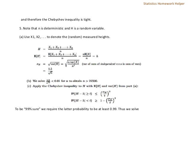
5. Define X as the height in meters of a randomly selected Canadian, where the selection probability is equal
for each Canadian, and denote E[X] by h. Bo is interested in estimating h. Because he is sure that no
Canadian is taller than 3 meters, Bo decides to use 1.5 meters as a conservative (large) value for the standard
deviation of X. To estimate h, Bo averages the heights of n Canadians that he selects at random; he denotes
this quantity by H.
(a) In terms of h and Bo’s 1.5 meter bound for the standard deviation of X, determine the expectation and
standard deviation for H.
(b) Help Bo by calculating a minimum value of n (with n > 0) such that the standard deviation of Bo’s
estimator, H, will be less than 0.01 meters.
(c) Say Bo would like to be 99% sure that his estimate is within 5 centimeters of the true average height of
Canadians. Using the Chebyshev inequality, calculate the minimum value of n that will make Bo happy.
(d) If we agree that no Canadians are taller than three meters, why is it correct to use 1.5 meters as an
upper bound on the standard deviation for X, the height of any Canadian selected at random?

6. Let X1, X2, . . . be independent, identically distributed, continuous random variables with E[X] = 2 and
var(X) = 9. Define Yi = (0.5)iXi , i = 1, 2, . . .. Also define Tn and An to be the sum and the average,
respectively, of the terms Y1, Y2, . . . , Yn.
(a) Is Yn convergent in probability? If so, to what value? Explain.
(b) Is Tn convergent in probability? If so, to what value? Explain.
(c) Is An convergent in probability? If so, to what value? Explain.
7. There are various senses of convergence for sequences of random variables. We have defined in
lecture “convergence in probability.” In this exercise, we will define “convergence in mean of order p.” (In
the case p = 2, it is called “mean square convergence.”) The sequence of random variables Y1, Y2, . . . is
said to converge in mean of order p (p > 0) to the real number a if
a) Prove that convergence in mean of order p (for any given positive value of p) implies convergence in
probability.
(b) Give a counterexample that shows that the converse is not true, i.e., convergence in probability does not
imply convergence in mean of order p.

G1† . One often needs to use sample data to estimate unknown parameters of the underlying distribution
from which samples are drawn. Examples of underlying parameters of interest include the mean and
variance of the distribution. In this problem, we look at estimators for mean and variance based on a set of n
observations X1, X2, . . . , Xn. If needed, assume that first, second, and fourth moment of the distribution are
finite. Denote an unknown parameter of interest by θ. An estimator is a function of the observed sample
data
that is used to estimate θ. An estimator is a function of random samples and, hence, a random variable
itself. To simplify the notation, we drop the argument of the estimator function. One desired property of an
estimator is unbiasedness. An estimator ˆθ is said to be unbiased when E[ ˆθ] = θ.
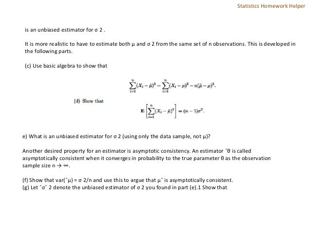
(a) Show that
is an unbiased estimator for the true mean µ.
(b) Now suppose that the mean µ is known but the variance σ 2 must be estimated from the sample. (The
more realistic situation with both µ and σ 2 unknown is considered below.) Show that

is an unbiased estimator for σ 2 .
It is more realistic to have to estimate both µ and σ 2 from the same set of n observations. This is developed in
the following parts.
(c) Use basic algebra to show that
e) What is an unbiased estimator for σ 2 (using only the data sample, not µ)?
Another desired property for an estimator is asymptotic consistency. An estimator ˆθ is called
asymptotically consistent when it converges in probability to the true parameter θ as the observation
sample size n → ∞.
(f) Show that var(ˆµ) = σ 2/n and use this to argue that µˆ is asymptotically consistent.
(g) Let ˆσˆ 2 denote the unbiased estimator of σ 2 you found in part (e).1 Show that

where d4 = E[(X − µ) 4 ]. Use this to argue that ˆσˆ 2 is asymptotically consistent.

Solutions
1. Let At (respectively, Bt) be a Bernoulli random variable that is equal to 1 if and only if the tth toss
resulted in 1 (respectively, 2). We have E[AtBt] = 0 (since At = 0 implies Bt = 0) and
2. (a) The minimum mean squared error estimator g(Y ) is known to be g(Y ) = E[X Y| ]. Let us first find fX,Y
(x, y). Since Y = X + W, we can write

and, therefore,
as shown in the plot below.
We now compute E[X Y ] by first determining fX Y | (x y). This can be done by | | looking at the
horizontal line crossing the compound PDF. Since fX,Y (x, y) is uniformly distributed in the defined
region, fX Y (x y) is uniformly distributed as well. Therefore,
The plot of g(y) is shown here.

(b) The linear least squares estimator has the form

The linear estimator gL(Y ) is compared with g(Y ) in the following figure. Note that g(Y ) is piecewise
linear in this problem
3. (a) The Chebyshev inequality yields P( X − 7 ≥ 3) ≤ 9 = 1, which implies the uninfor- 3 | | 2
mative/useless bound P(4 < X < 10) ≥ 0.
(b) We will show that P(4 < X < 10) can be as small as 0 and can be arbitrarily close to 1. Consider a
random variable that equals 4 with probability 1/2, and 10 with probability 1/2. This random variable has
mean 7 and variance 9, and P(4 < X < 10) = 0. Therefore, the lower bound from part (a) is the best
possible. Let us now fix a small positive number ǫ and another positive number c, and consider a discrete
random variable X with PMF

This random variable has a mean of 7. Its variance is
and can be made equal to 9 by suitably choosing c. For this random variable, we have P(4 < X < 10) = 1 −
2ǫ, which can be made arbitrarily close to 1. On the other hand, this probability can not be made equal to
1. Indeed, if this probability were equal to 1, then we would have | | X − 7 ≤ 3, which would imply that the
variance in less than 9.
4. Consider a random variable X with PMF

and therefore the Chebyshev inequality is tight.
5. Note that n is deterministic and H is a random variable.
(a) Use X1, X2, . . . to denote the (random) measured heights.
To be “99% sure” we require the latter probability to be at least 0.99. Thus we solve

(d) The variance of a random variable increases as its distribution becomes more spread out. In particular,
if a random variable is known to be limited to a particular closed interval, the variance is maximized by
having 0.5 probability of taking on each endpoint value. In this problem, random variable X has an
unknown distribution over [0, 3]. The variance of X cannot be more than the variance of a random
variable that equals 0 with probability 0.5 and 3 with probability 0.5. This translates to the standard
deviation not exceeding 1.5. In fact, this argument can be made more rigorous as follows. First, we have
since E[(X − a)2] is minimized when a is the mean (i.e., the mean is the least-squared estimator).
Second, we also have

since the variable has support in [0, 3]. Adding the above two inequalities, we have
6. First, let’s calculate the expectation and the variance for Yn, Tn, and An.

(a) Yes. Yn converges to 0 in probability. As n becomes very large, the expected value of Yn approaches 0 and
the variance of Yn approaches 0. So, by the Chebychev Inequality, Yn converges to 0 in probability.
(b) No. Assume that Tn converges in probability to some value a. We also know that:
2 Notice that 0.5X2 + (0.5)2X3 + 5) · · · + (0. n−1Xn converges to the same limit as Tn when n goes to infinity.
If Tn is to converge to a, Y1 must converge to a/2. But this is clearly false, which presents a contradiction in
our original assumption.
(c) Yes. An converges to 0 in probability. As n becomes very large, the expected value of An approaches 0,
and the variance of An approaches 0. So, by the Chebychev Inequality, An converges to 0 in probability. You
could also show this by noting that the Ans are i.i.d. with finite mean and variance and using the WLLN.
7. (a) Suppose Y1, Y2, . . . converges to a in mean of order p. This means that E[ Yn −a p | | ] → 0, so to
prove convergence in probability we should upper bound P(| | Yn − a ≥ ǫ) by a multiple of E[ Yn − a p | |
]. This connection is provided by the Markov inequality. Let ǫ > 0 and note the bound

where the first step is a manipulation that does not change the event under consideration and the second
step is the Markov inequality applied to the random variable . Since the inequality above holds for
every n,
Hence, we have that converges in probability to a.
(b) Consider the sequence of random variables where
Therefore ˆσ2 (which uses the true mean) is unbiased estimator for σ2.

is an unbiased estimator for the variance.
Thus, var(ˆµ) goes to zero asymptotically. Furthermore, we saw that E[ˆµ] = µ. Simple application of
Chebyshev inequality shows that ˆµ converges in probability to µ (the true mean) as the sample size
increases.
(g) Not yet typeset.

Statistics Homework Help

More Related Content

Similar to Statistics Homework Help

More from Statistics Homework Helper

Recently uploaded

Statistics Homework Help