The field aims to understand natural systems, human impacts, and to develop solutions for sdlc ,water fall model

1. Project Management Concepts
 Management Spectrum
1

2. 2
The Four P’s
 People — the most important element of a
successful project
 Product — the software to be built
 Process — the set of framework activities and
software engineering tasks to get the job done
 Project — all work required to make the
product a reality

3. 3
Stakeholders
 Senior managers who define the business issues that
often have significant influence on the project.
 Project (technical) managers who must plan, motivate,
organize, and control the practitioners who do software
work.
 Practitioners who deliver the technical skills that are
necessary to engineer a product or application.
 Customers who specify the requirements for the software
to be engineered and other stakeholders who have a
peripheral interest in the outcome.
 End-users who interact with the software once it is
released for production use.

4. 4
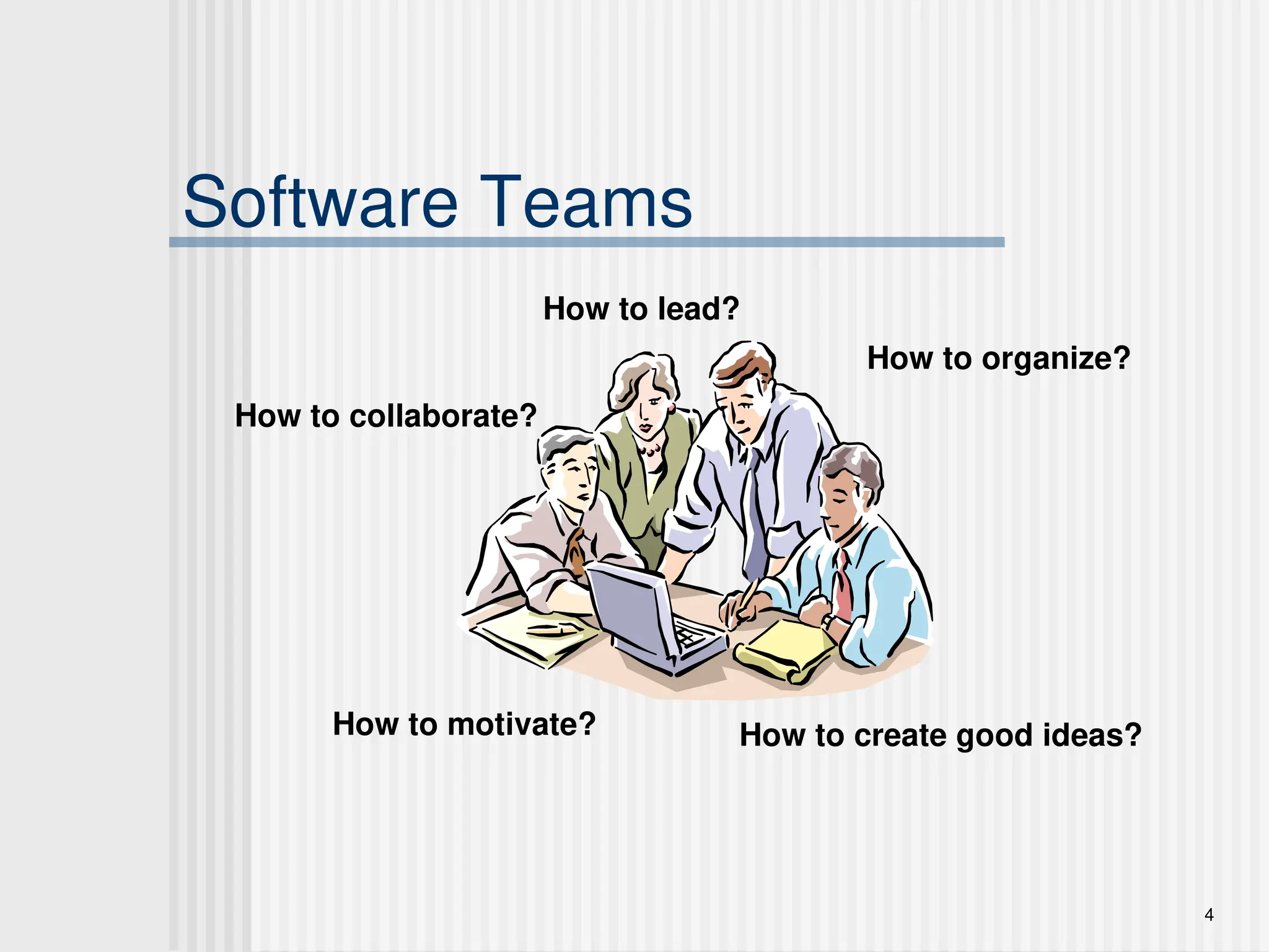
Software Teams
How to lead?
How to organize?
How to motivate?
How to collaborate?
How to create good ideas?

5. 5
Team Leader
 The MOI Model
 Motivation. The ability to encourage (by “push or
pull”) technical people to produce to their best ability.
 Organization. The ability to mold existing processes
(or invent new ones) that will enable the initial
concept to be translated into a final product.
 Ideas or innovation. The ability to encourage
people to create and feel creative even when they
must work within bounds established for a particular
software product or application.

6. 6
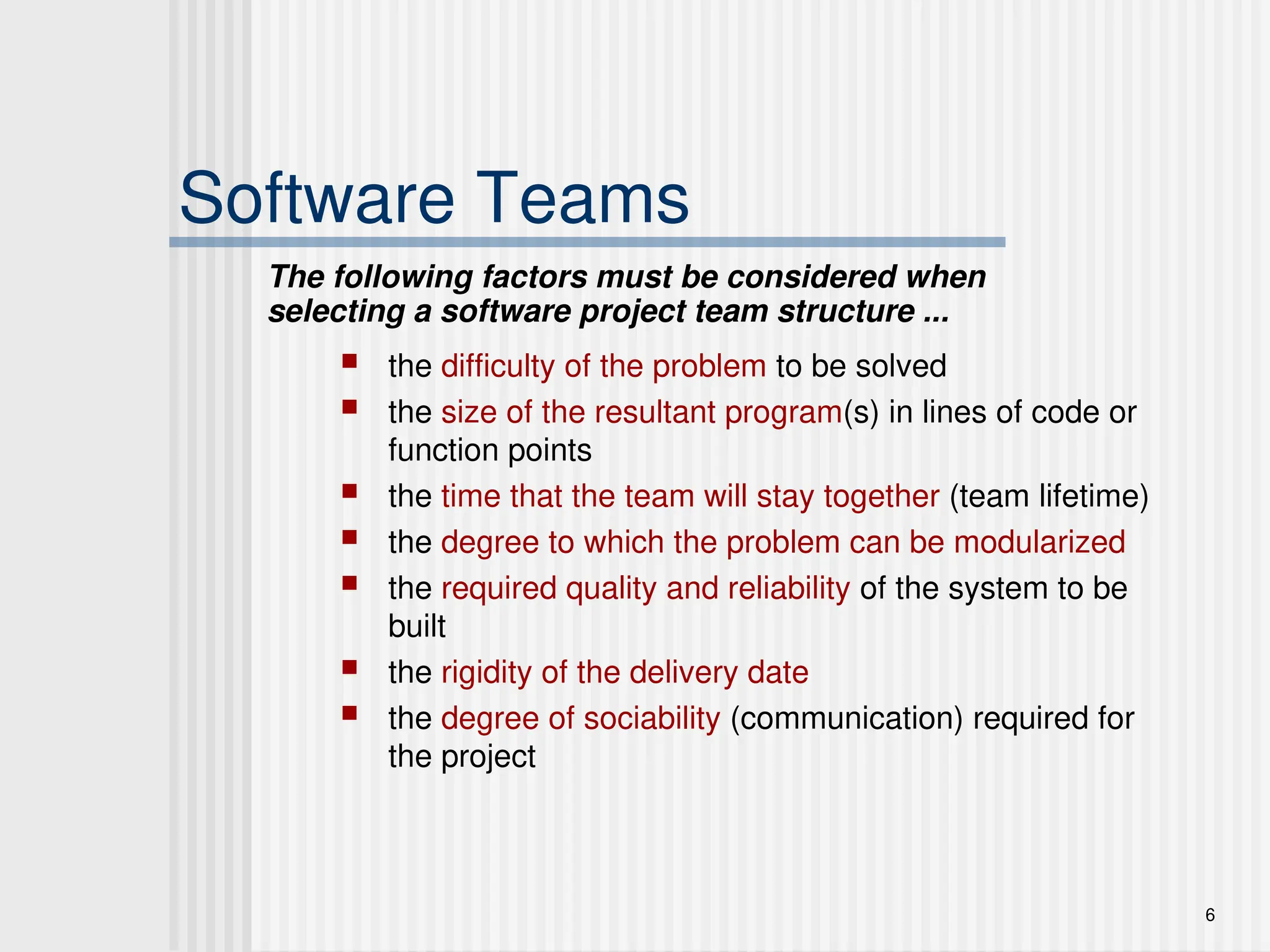
Software Teams
 the difficulty of the problem to be solved
 the size of the resultant program(s) in lines of code or
function points
 the time that the team will stay together (team lifetime)
 the degree to which the problem can be modularized
 the required quality and reliability of the system to be
built
 the rigidity of the delivery date
 the degree of sociability (communication) required for
the project
The following factors must be considered when
selecting a software project team structure ...

7. 7
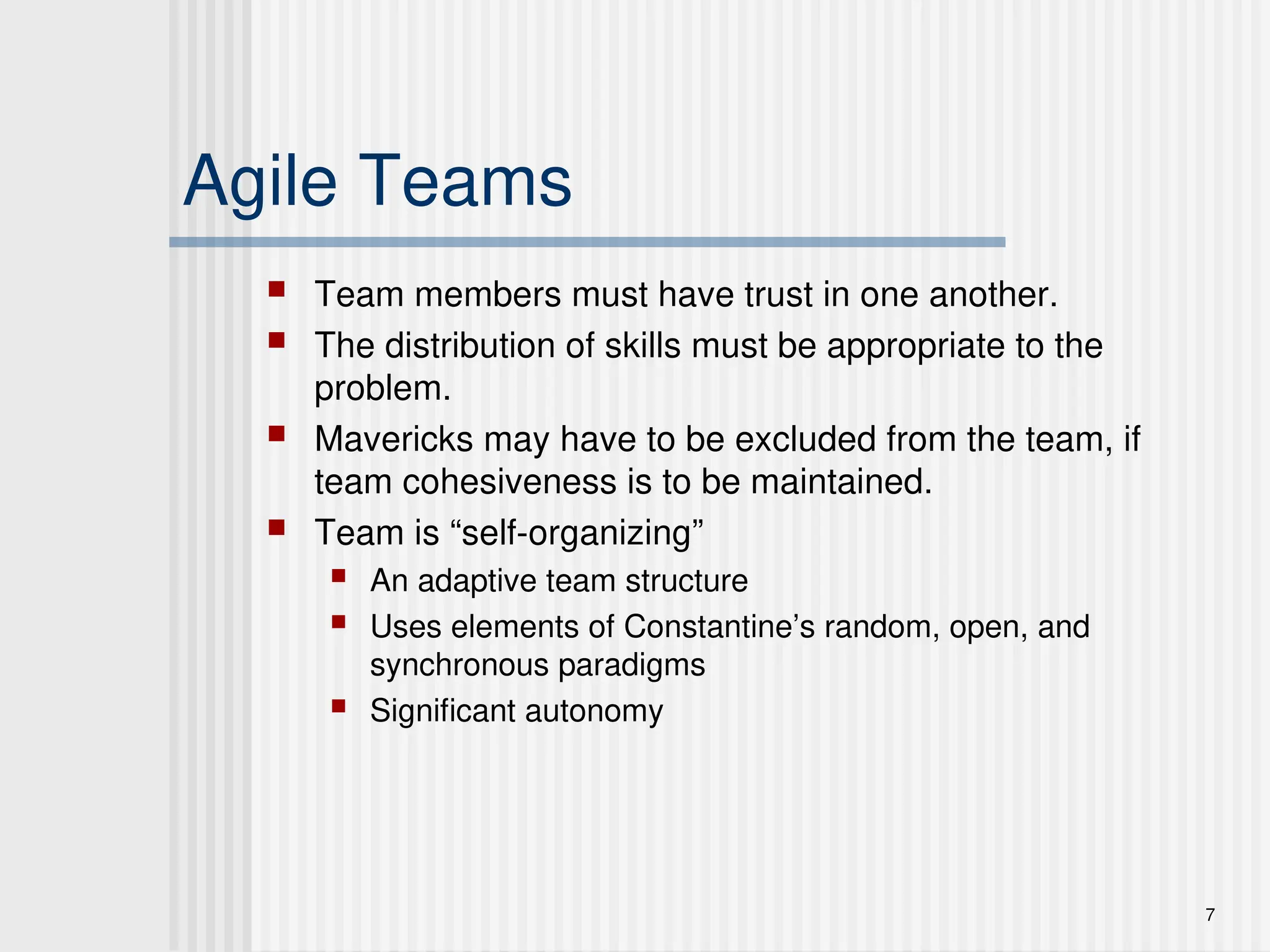
Agile Teams
 Team members must have trust in one another.
 The distribution of skills must be appropriate to the
problem.
 Mavericks may have to be excluded from the team, if
team cohesiveness is to be maintained.
 Team is “self-organizing”
 An adaptive team structure
 Uses elements of Constantine’s random, open, and
synchronous paradigms
 Significant autonomy

8. 8
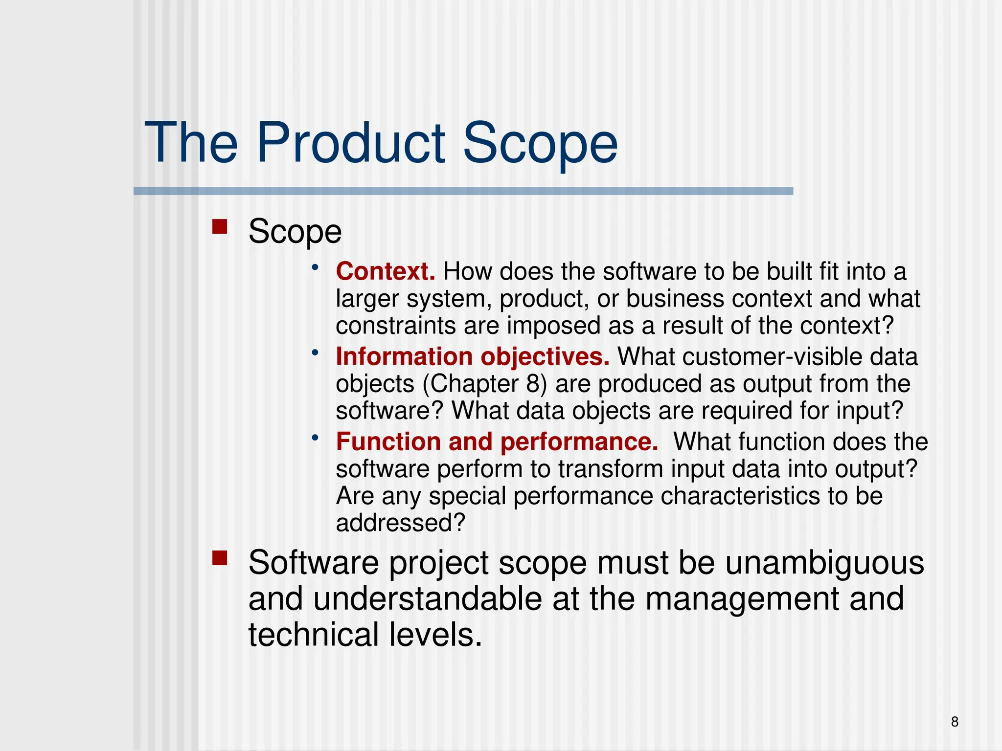
The Product Scope
 Scope
• Context. How does the software to be built fit into a
larger system, product, or business context and what
constraints are imposed as a result of the context?
• Information objectives. What customer-visible data
objects (Chapter 8) are produced as output from the
software? What data objects are required for input?
• Function and performance. What function does the
software perform to transform input data into output?
Are any special performance characteristics to be
addressed?
 Software project scope must be unambiguous
and understandable at the management and
technical levels.

9. 9
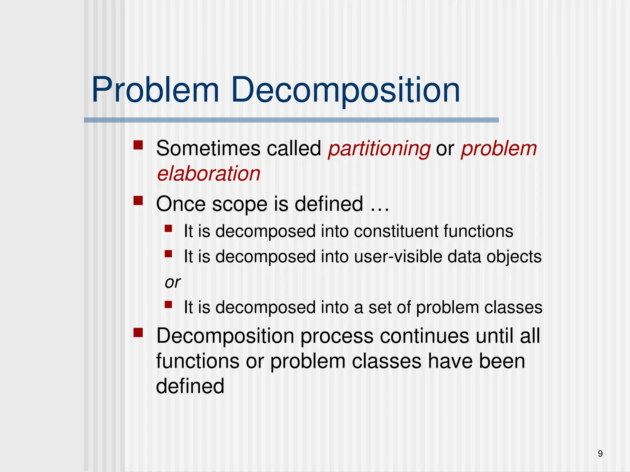
Problem Decomposition
 Sometimes called partitioning or problem
elaboration
 Once scope is defined …
 It is decomposed into constituent functions
 It is decomposed into user-visible data objects
or
 It is decomposed into a set of problem classes
 Decomposition process continues until all
functions or problem classes have been
defined

10. 10
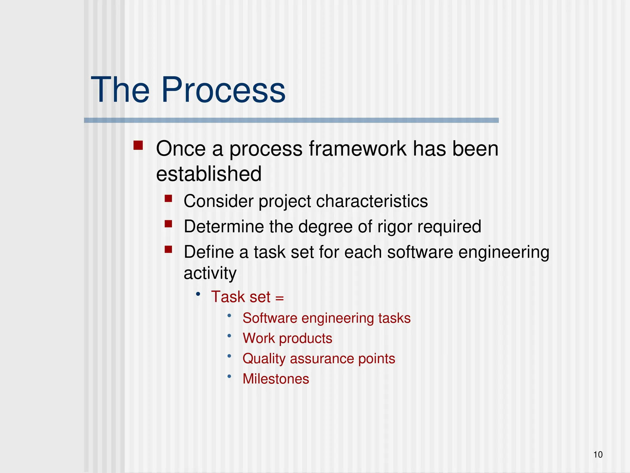
The Process
 Once a process framework has been
established
 Consider project characteristics
 Determine the degree of rigor required
 Define a task set for each software engineering
activity
• Task set =
• Software engineering tasks
• Work products
• Quality assurance points
• Milestones

11. 11
Melding the Problem and the Process

12. 12
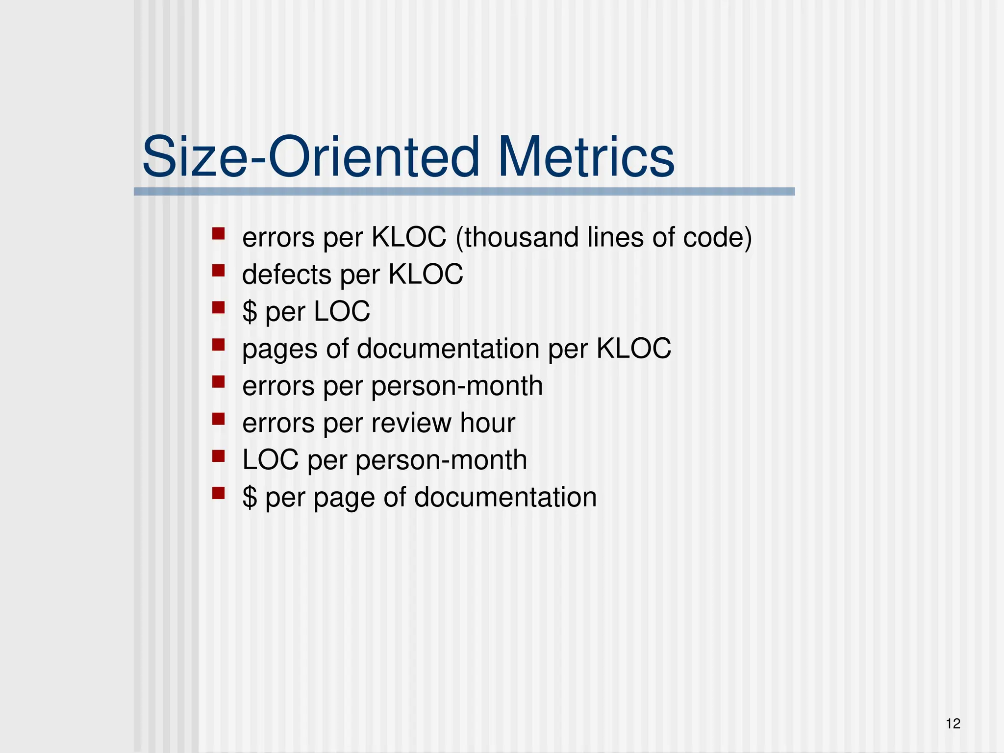
Size-Oriented Metrics
 errors per KLOC (thousand lines of code)
 defects per KLOC
 $ per LOC
 pages of documentation per KLOC
 errors per person-month
 errors per review hour
 LOC per person-month
 $ per page of documentation

13. 13
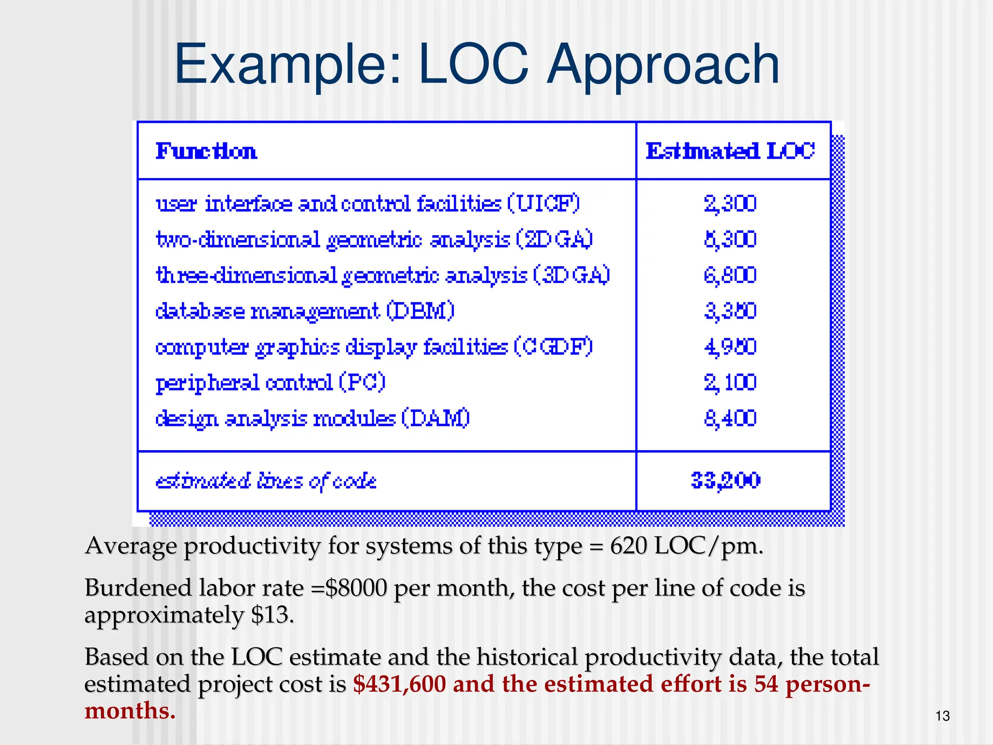
Example: LOC Approach
Average productivity for systems of this type = 620 LOC/pm.
Average productivity for systems of this type = 620 LOC/pm.
Burdened labor rate =$8000 per month, the cost per line of code is
Burdened labor rate =$8000 per month, the cost per line of code is
approximately $13.
approximately $13.
Based on the LOC estimate and the historical productivity data, the total
Based on the LOC estimate and the historical productivity data, the total
estimated project cost is
estimated project cost is $431,600 and the estimated effort is 54 person-
months.

14. 14
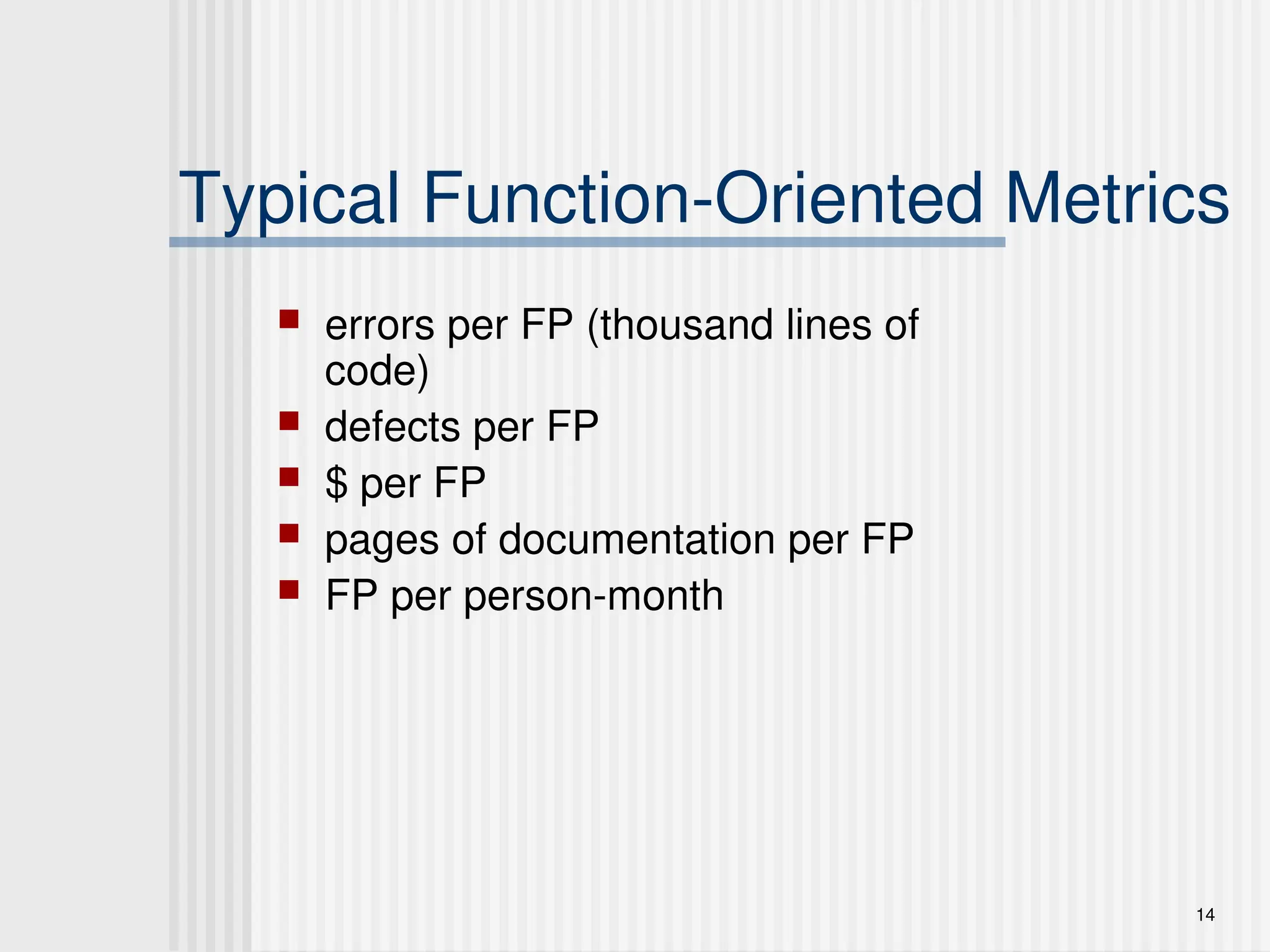
Typical Function-Oriented Metrics
 errors per FP (thousand lines of
code)
 defects per FP
 $ per FP
 pages of documentation per FP
 FP per person-month

15. 15
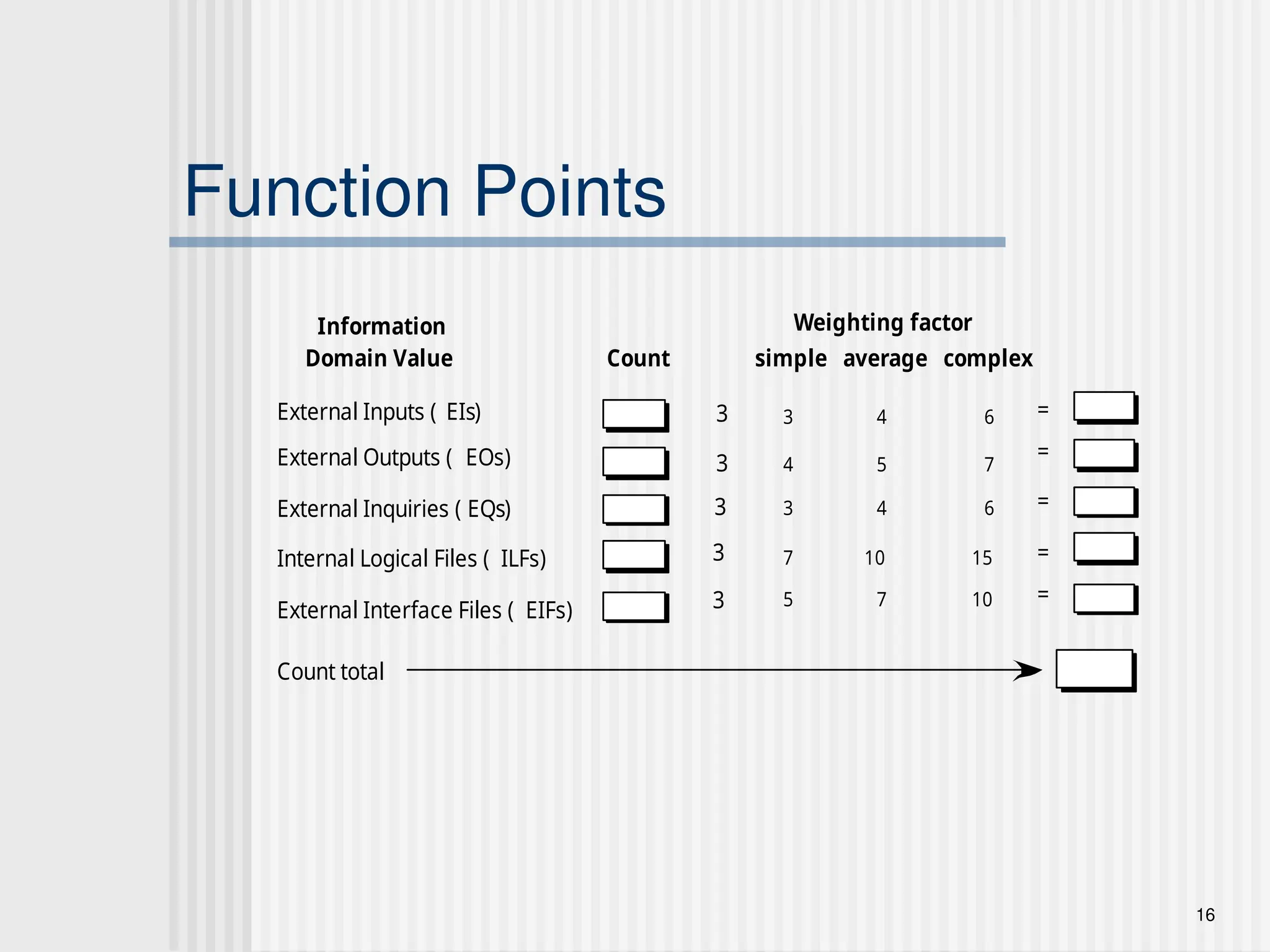
Function-Based Metrics
 The function point metric (FP), first proposed by Albrecht [ALB79],
can be used effectively as a means for measuring the functionality
delivered by a system.
 Function points are derived using an empirical relationship based
on countable (direct) measures of software's information domain
and assessments of software complexity
 Information domain values are defined in the following manner:
 number of external inputs (EIs)
 number of external outputs (EOs)
 number of external inquiries (EQs)
 number of internal logical files (ILFs)
 Number of external interface files (EIFs)

16. 16
Function Points
Information
Domain Value Count simple average complex
Weighting factor
External Inputs ( EIs)
External Outputs ( EOs)
External Inquiries ( EQs)
Internal Logical Files ( ILFs)
External Interface Files ( EIFs)
3 4 6
4 5 7
3 4 6
7 10 15
5 7 10
=
=
=
=
=
Count total
3
3
3
3
3

17. 17
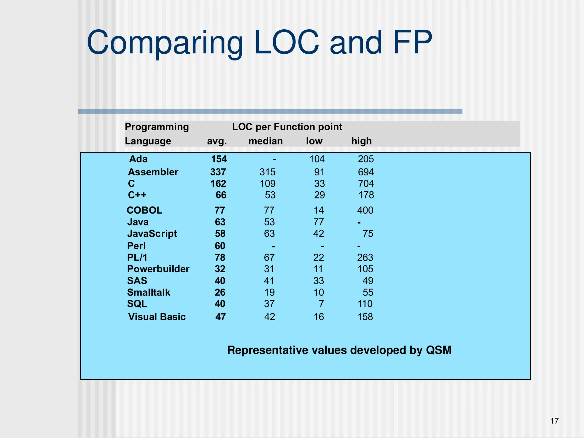
Comparing LOC and FP
Programming LOC per Function point
Language avg. median low high
Ada 154 - 104 205
Assembler 337 315 91 694
C 162 109 33 704
C++ 66 53 29 178
COBOL 77 77 14 400
Java 63 53 77 -
JavaScript 58 63 42 75
Perl 60 - - -
PL/1 78 67 22 263
Powerbuilder 32 31 11 105
SAS 40 41 33 49
Smalltalk 26 19 10 55
SQL 40 37 7 110
Visual Basic 47 42 16 158
Representative values developed by QSM

18. 18
Example: FP Approach
The estimated number of FP is derived:
The estimated number of FP is derived:
FP
FPestimated
estimated = count-total [0.65 + 0.01
= count-total [0.65 + 0.01 3
3 S
S (F
(Fi
i)]
)]
FP
FPestimated
estimated = 375
= 375
organizational average productivity = 6.5 FP/pm.
organizational average productivity = 6.5 FP/pm.
burdened labor rate = $8000 per month, approximately $1230/FP.
burdened labor rate = $8000 per month, approximately $1230/FP.
Based on the FP estimate and the historical productivity data,
Based on the FP estimate and the historical productivity data, total estimated project
cost is $461,250 and estimated effort is 58 person-months.

19. 19
Why Opt for FP?
 Programming language independent
 Used readily countable characteristics that
are determined early in the software process
 Does not “penalize” inventive (short)
implementations that use fewer LOC that
other more clumsy versions
 Makes it easier to measure the impact of
reusable components

20. 20
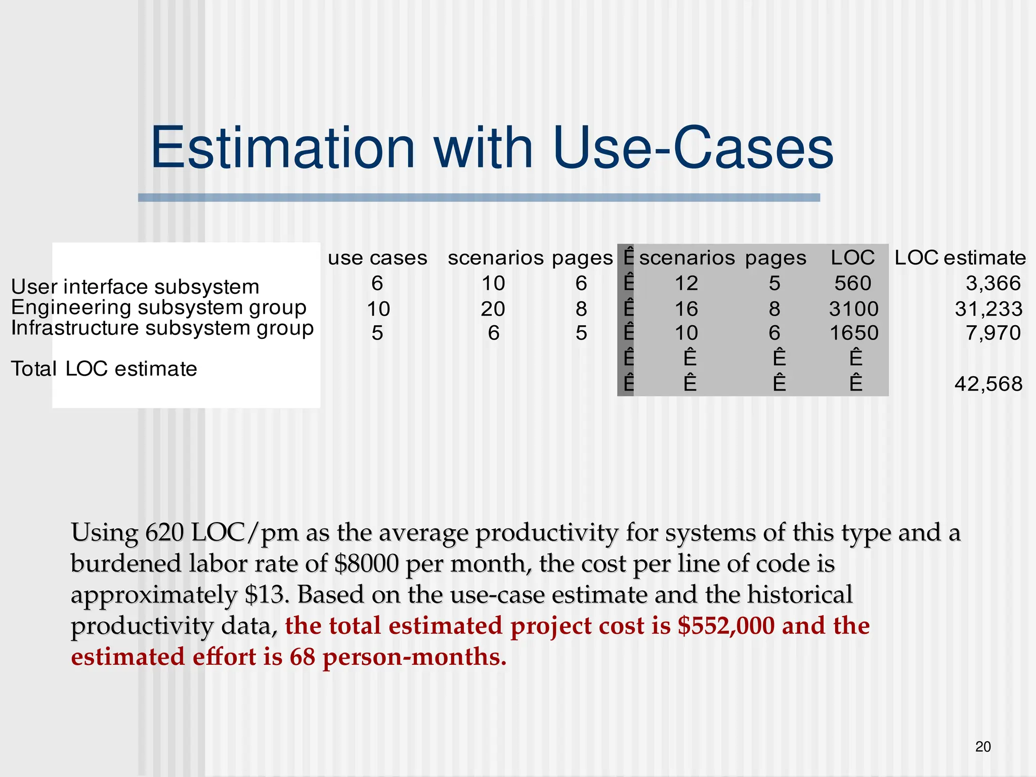
Estimation with Use-Cases
use cases scenarios pages Êscenarios pages LOC LOC estimate
e subsystem 6 10 6 Ê 12 5 560 3,366
subsystem group 10 20 8 Ê 16 8 3100 31,233
e subsystem group 5 6 5 Ê 10 6 1650 7,970
Ê Ê Ê Ê
stimate Ê Ê Ê Ê 42,568
User interface subsystem
Engineering subsystem group
Infrastructure subsystem group
Total LOC estimate
Using 620 LOC/pm as the average productivity for systems of this type and a
Using 620 LOC/pm as the average productivity for systems of this type and a
burdened labor rate of $8000 per month, the cost per line of code is
burdened labor rate of $8000 per month, the cost per line of code is
approximately $13. Based on the use-case estimate and the historical
approximately $13. Based on the use-case estimate and the historical
productivity data,
productivity data, the total estimated project cost is $552,000 and the
estimated effort is 68 person-months.

21. 21
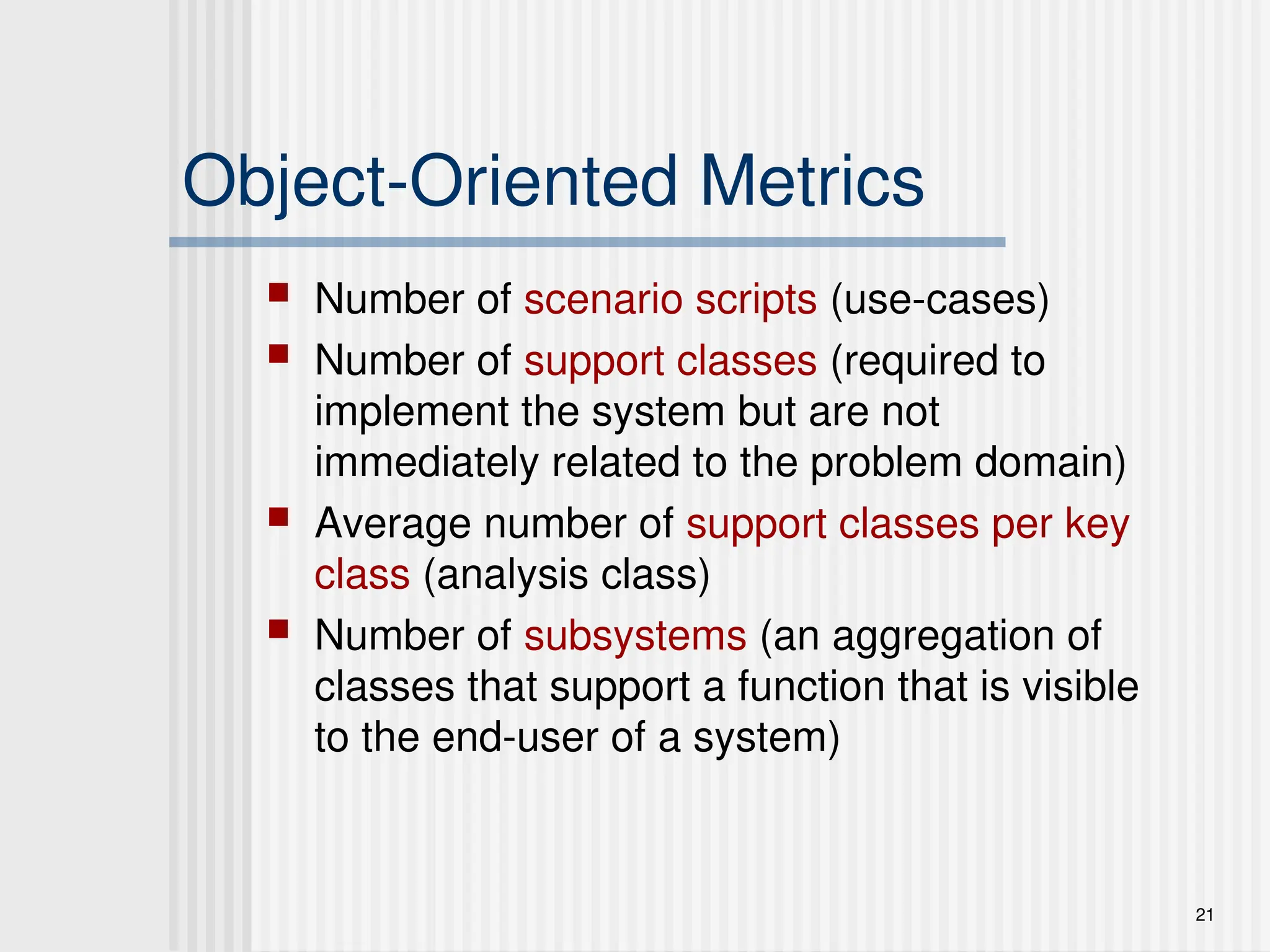
Object-Oriented Metrics
 Number of scenario scripts (use-cases)
 Number of support classes (required to
implement the system but are not
immediately related to the problem domain)
 Average number of support classes per key
class (analysis class)
 Number of subsystems (an aggregation of
classes that support a function that is visible
to the end-user of a system)

22. 22
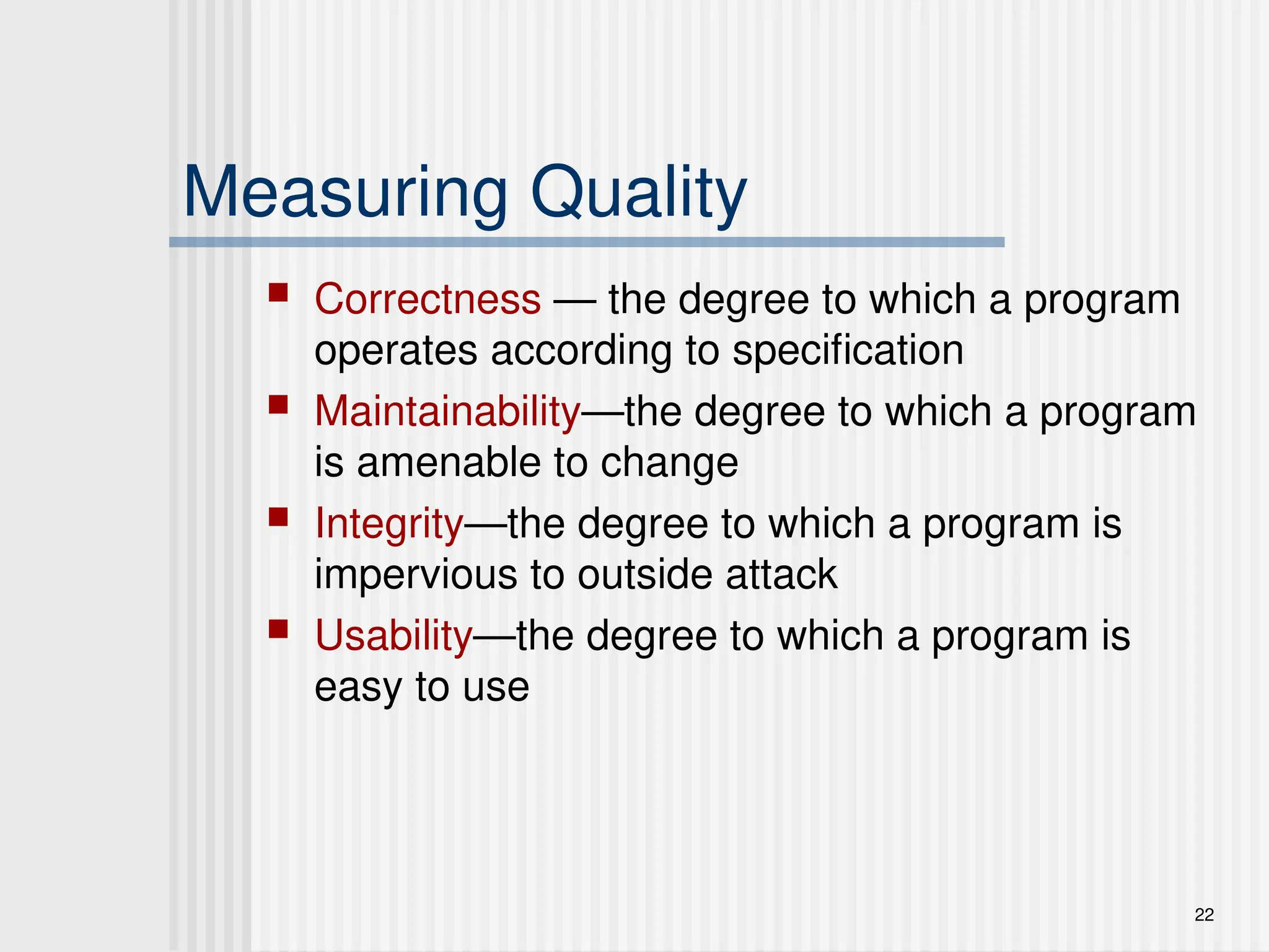
Measuring Quality
 Correctness — the degree to which a program
operates according to specification
 Maintainability—the degree to which a program
is amenable to change
 Integrity—the degree to which a program is
impervious to outside attack
 Usability—the degree to which a program is
easy to use

23. 23
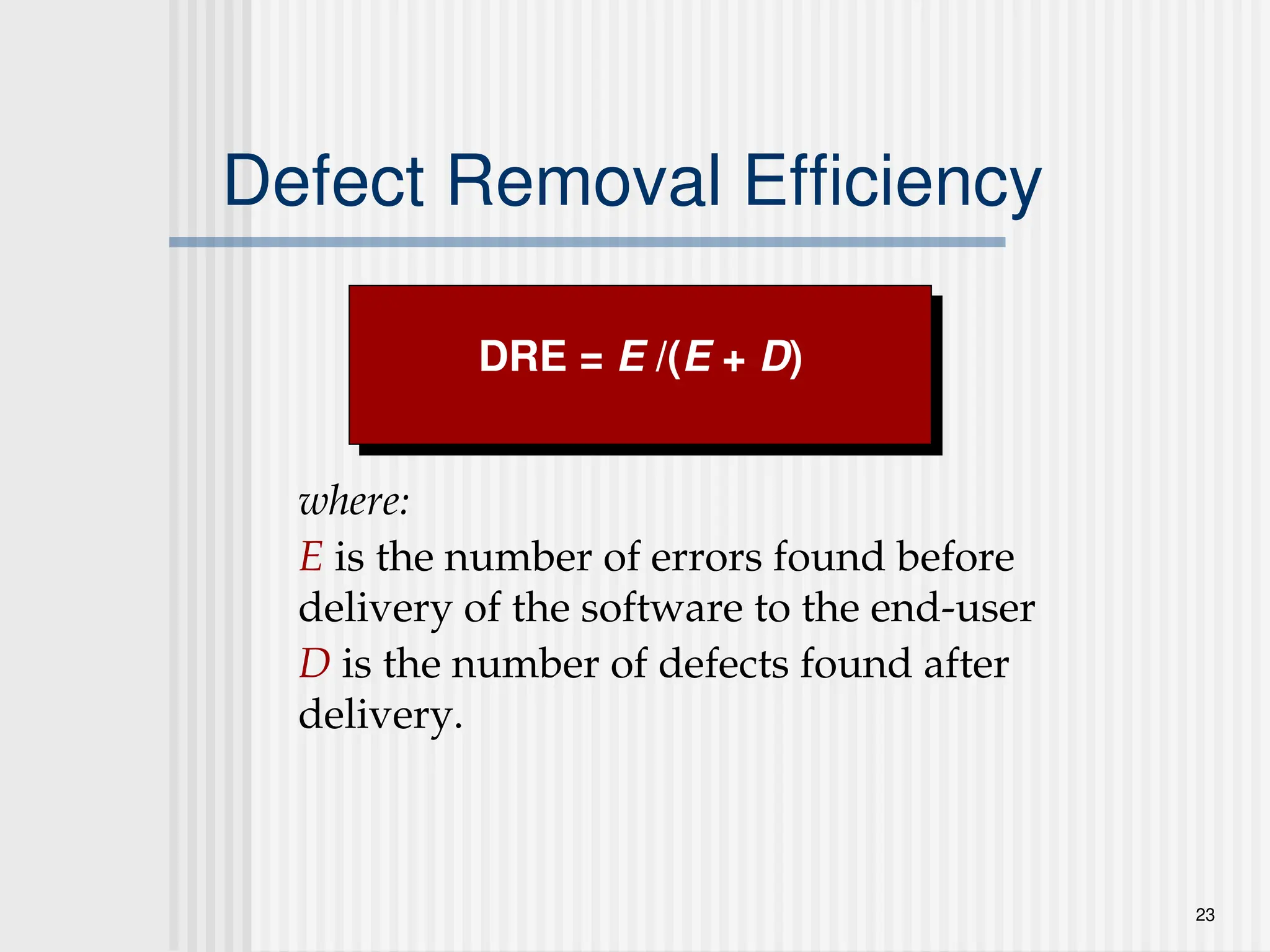
Defect Removal Efficiency
where:
E is the number of errors found before
delivery of the software to the end-user
D is the number of defects found after
delivery.
DRE = E /(E + D)

24. 24
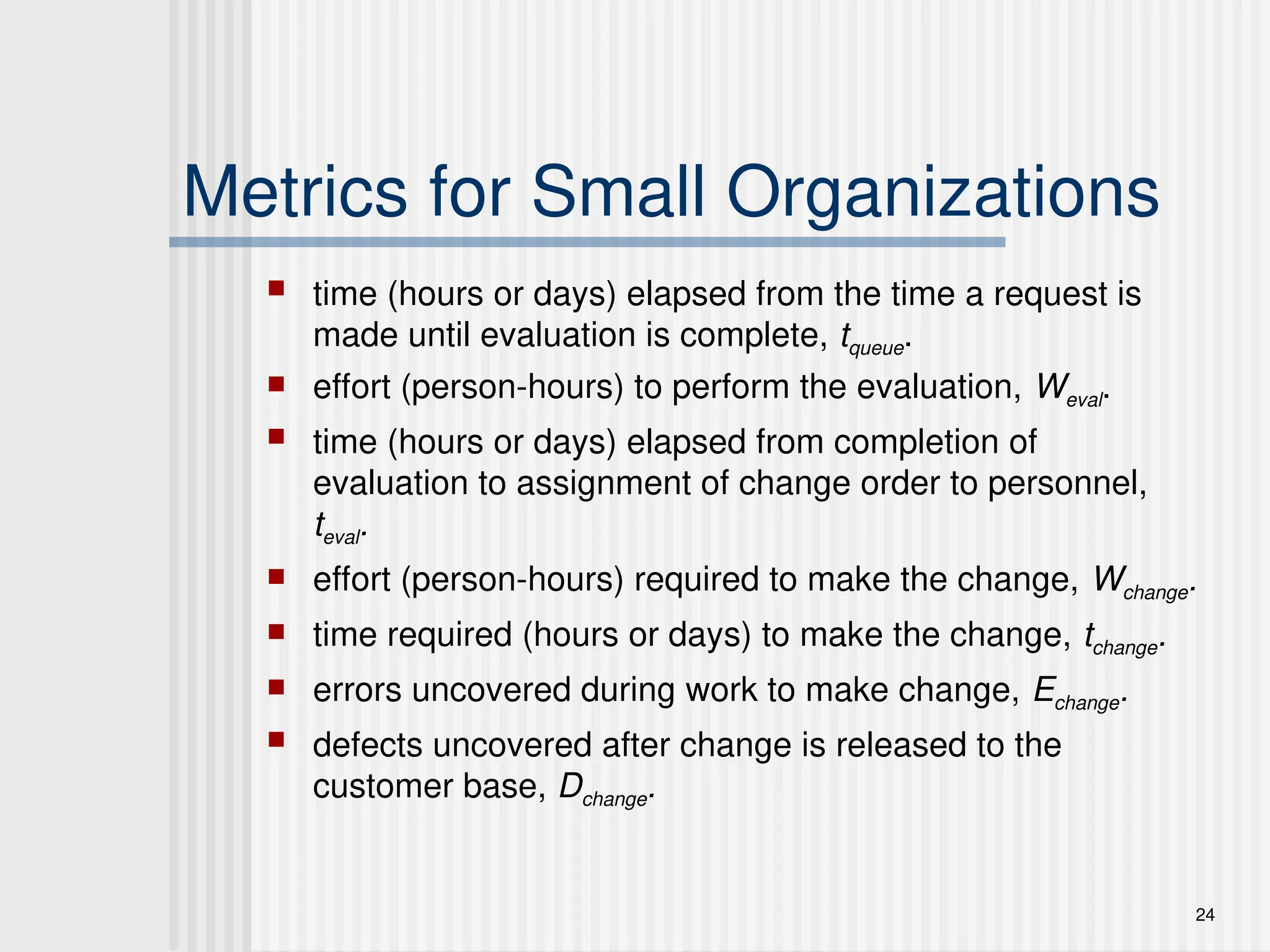
Metrics for Small Organizations
 time (hours or days) elapsed from the time a request is
made until evaluation is complete, tqueue.
 effort (person-hours) to perform the evaluation, Weval.
 time (hours or days) elapsed from completion of
evaluation to assignment of change order to personnel,
teval.
 effort (person-hours) required to make the change, Wchange.
 time required (hours or days) to make the change, tchange.
 errors uncovered during work to make change, Echange.
 defects uncovered after change is released to the
customer base, Dchange.

25. 25
Establishing a Metrics Program
 Identify your business goals.
 Identify what you want to know or learn.
 Identify your subgoals.
 Identify the entities and attributes related to your subgoals.
 Formalize your measurement goals.
 Identify quantifiable questions and the related indicators that
you will use to help you achieve your measurement goals.
 Identify the data elements that you will collect to construct
the indicators that help answer your questions.
 Define the measures to be used, and make these definitions
operational.
 Identify the actions that you will take to implement the
measures.
 Prepare a plan for implementing the measures.

26. 26
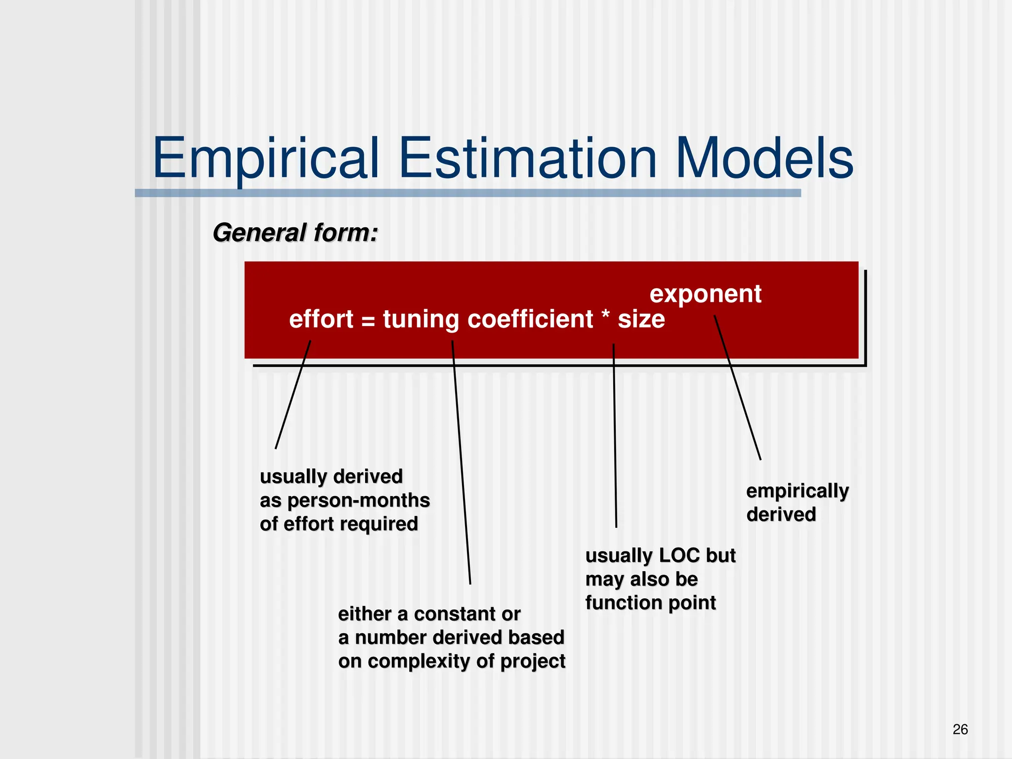
Empirical Estimation Models
General form:
General form:
effort = tuning coefficient * size
exponent
usually derived
usually derived
as person-months
as person-months
of effort required
of effort required
either a constant or
either a constant or
a number derived based
a number derived based
on complexity of project
on complexity of project
usually LOC but
usually LOC but
may also be
may also be
function point
function point
empirically
empirically
derived
derived

27. 26/12/2016
27
Introduction to COCOMO
models
 The COstructive COst Model (COCOMO) is
the most widely used software estimation
model.
 The COCOMO model predicts the effort and
duration of a project based on inputs relating
to the size of the resulting systems and a
number of "cost drives" that affect
productivity.

28. 26/12/2016
28
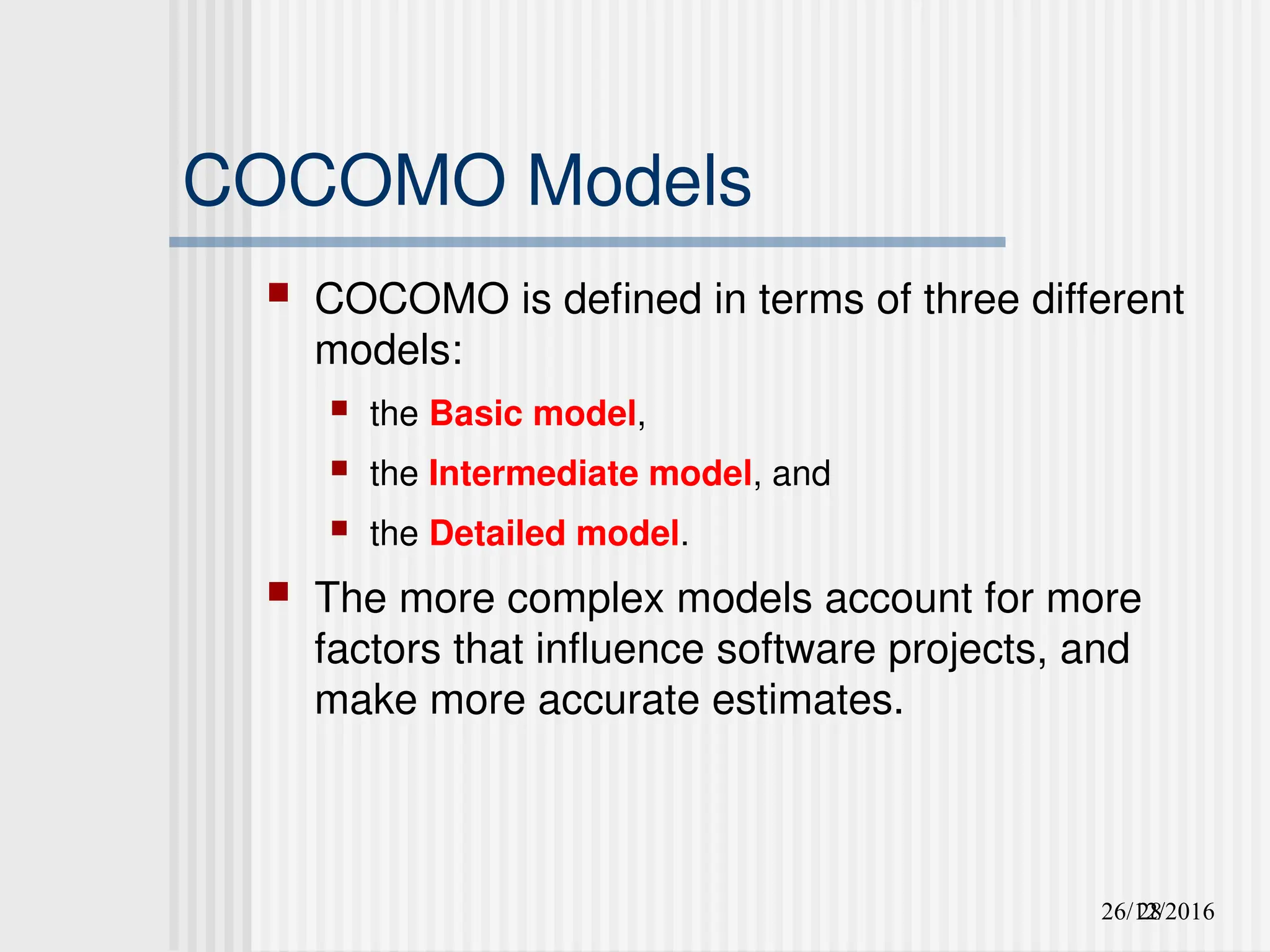
COCOMO Models
 COCOMO is defined in terms of three different
models:
 the Basic model,
 the Intermediate model, and
 the Detailed model.
 The more complex models account for more
factors that influence software projects, and
make more accurate estimates.

29. 26/12/2016
29
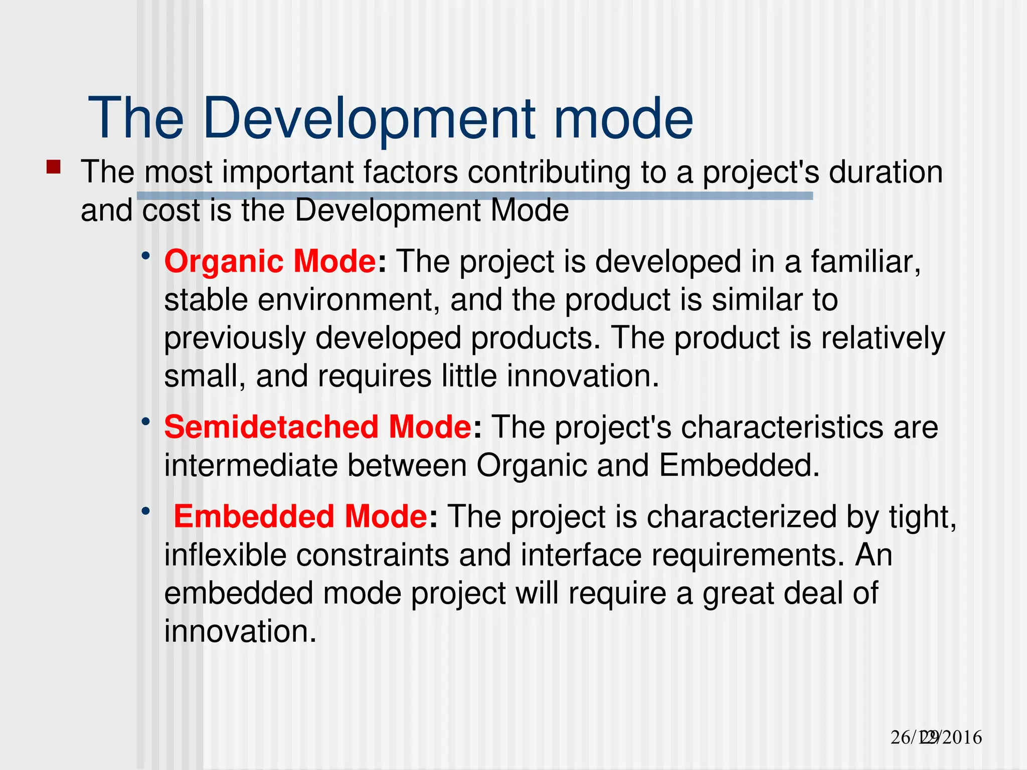
The Development mode
 The most important factors contributing to a project's duration
and cost is the Development Mode
• Organic Mode: The project is developed in a familiar,
stable environment, and the product is similar to
previously developed products. The product is relatively
small, and requires little innovation.
• Semidetached Mode: The project's characteristics are
intermediate between Organic and Embedded.
• Embedded Mode: The project is characterized by tight,
inflexible constraints and interface requirements. An
embedded mode project will require a great deal of
innovation.

30. 26/12/2016
30
Modes

31. 26/12/2016
31
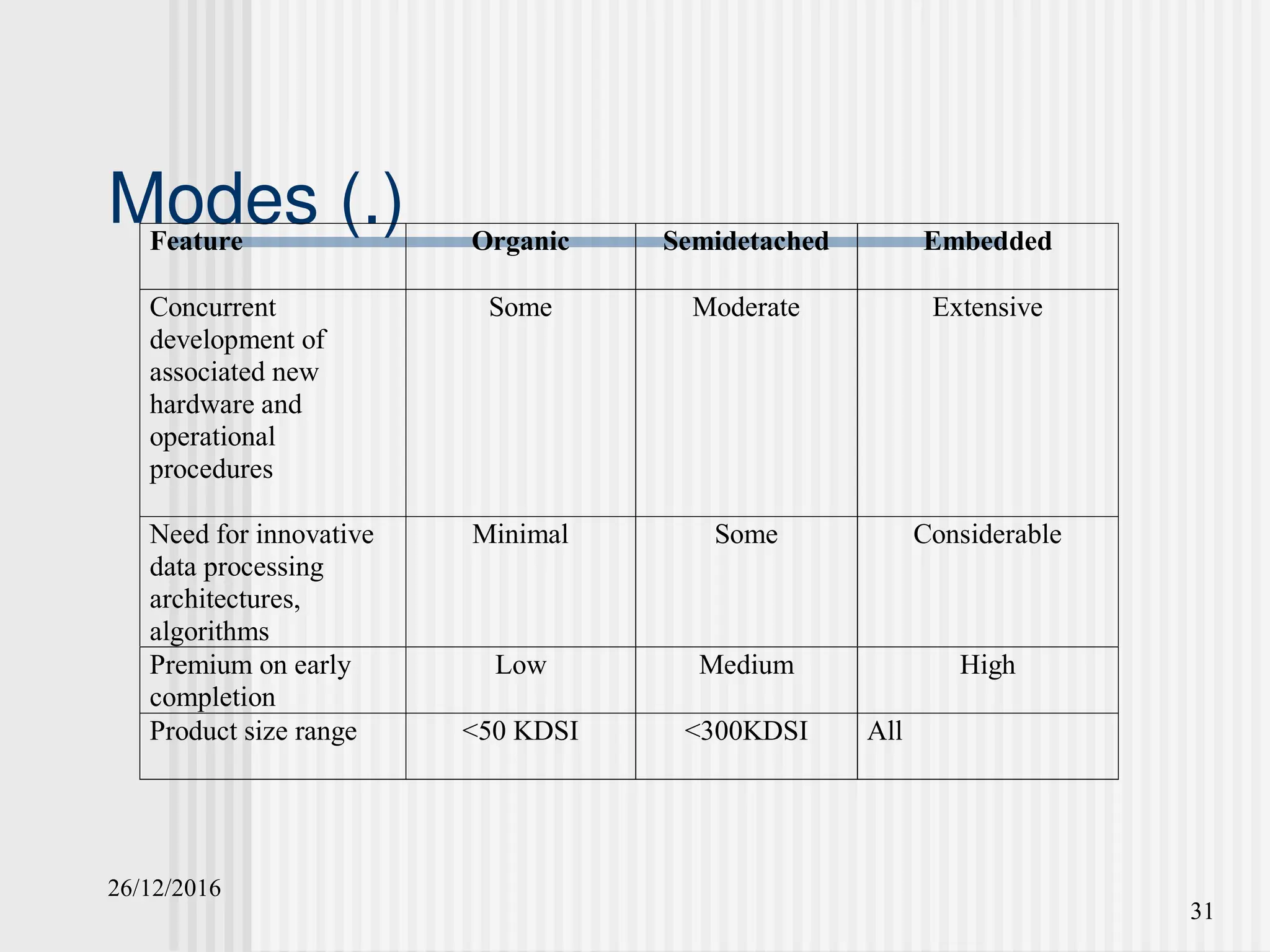
Modes (.)
Feature Organic Semidetached Embedded
Concurrent
development of
associated new
hardware and
operational
procedures
Some Moderate Extensive
Need for innovative
data processing
architectures,
algorithms
Minimal Some Considerable
Premium on early
completion
Low Medium High
Product size range <50 KDSI <300KDSI All

32. 26/12/2016
32
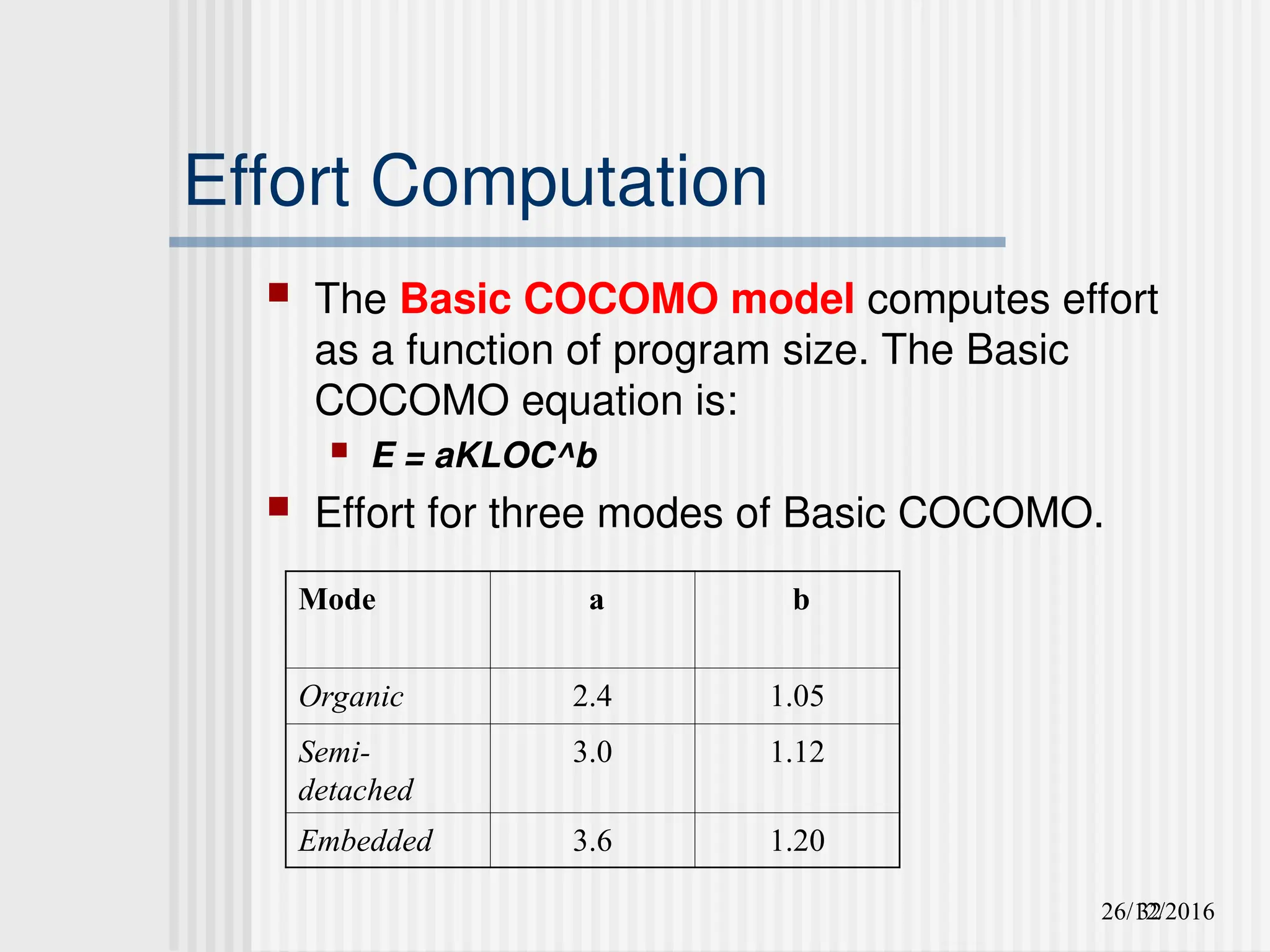
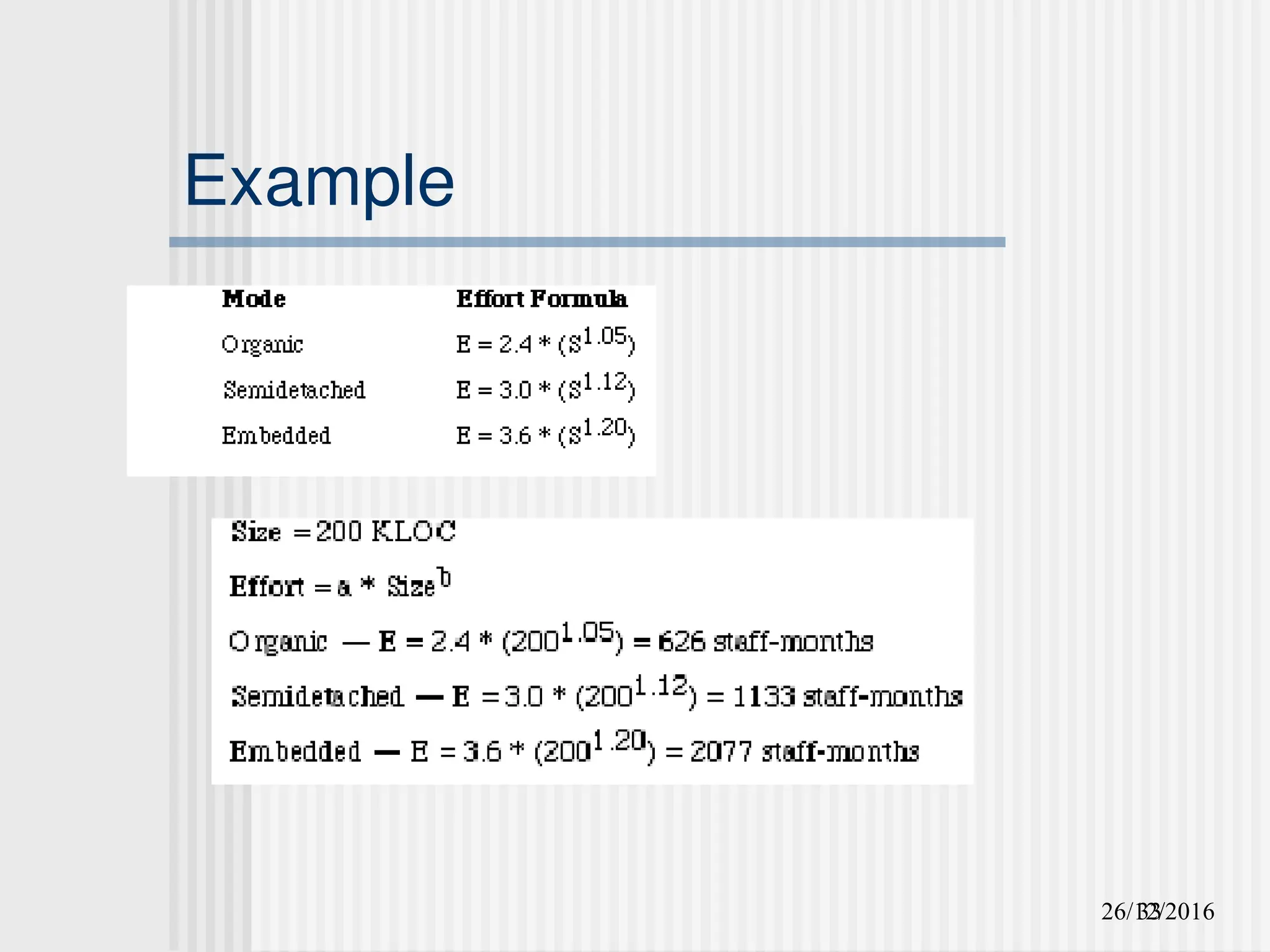
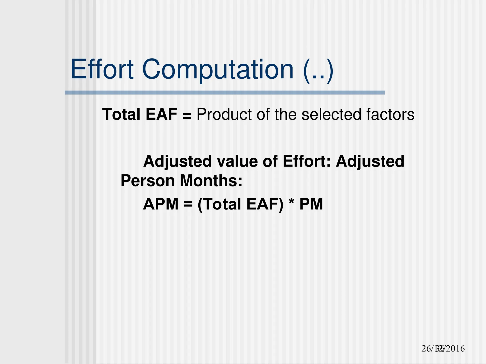
Effort Computation
 The Basic COCOMO model computes effort
as a function of program size. The Basic
COCOMO equation is:
 E = aKLOC^b
 Effort for three modes of Basic COCOMO.
Mode a b
Organic 2.4 1.05
Semi-
detached
3.0 1.12
Embedded 3.6 1.20

33. 26/12/2016
33
Example

34. 26/12/2016
34
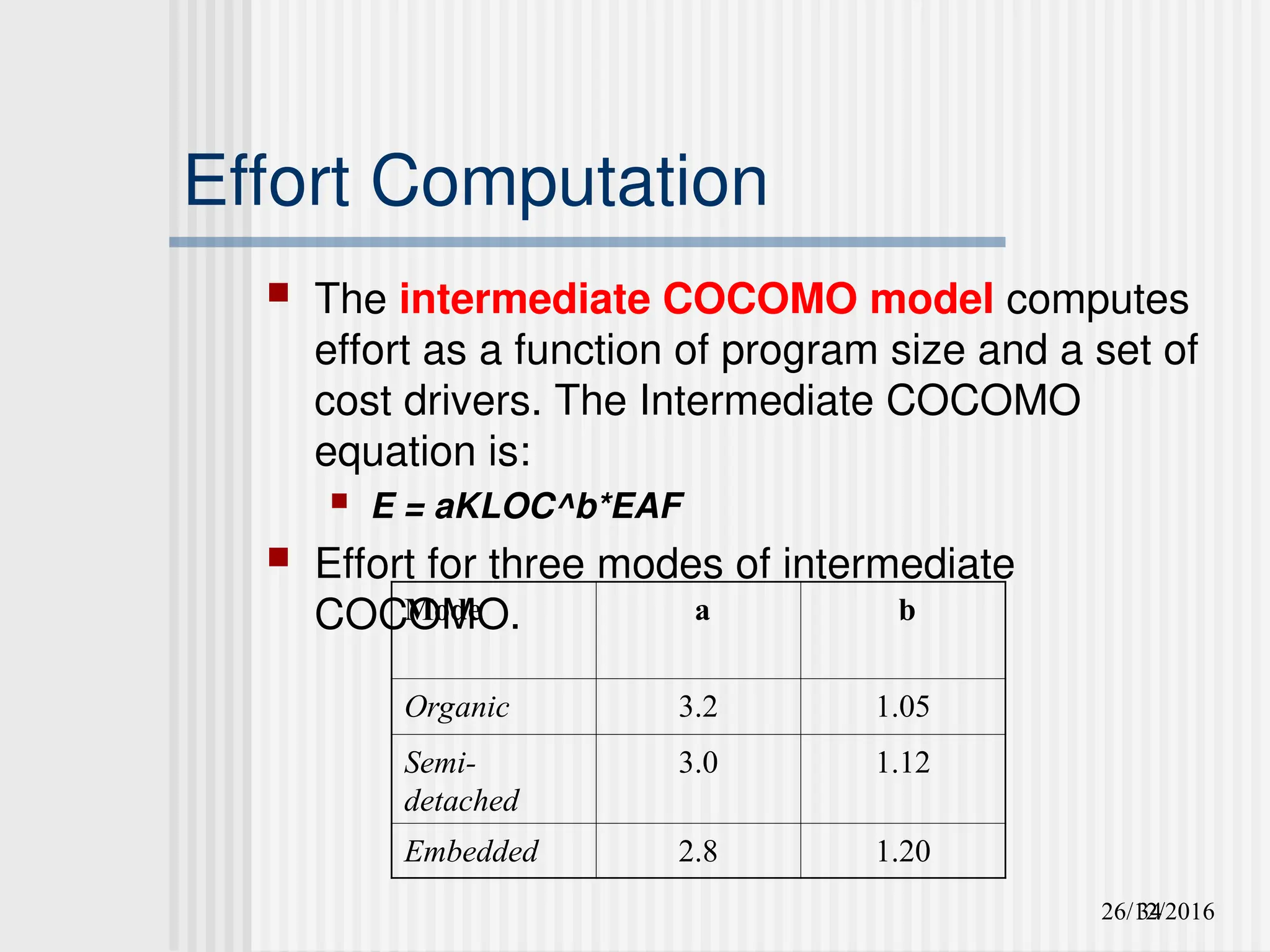
Effort Computation
 The intermediate COCOMO model computes
effort as a function of program size and a set of
cost drivers. The Intermediate COCOMO
equation is:
 E = aKLOC^b*EAF
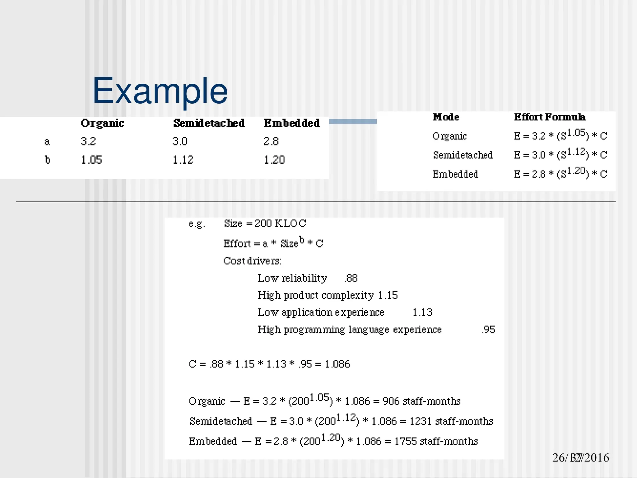
 Effort for three modes of intermediate
COCOMO.
Mode a b
Organic 3.2 1.05
Semi-
detached
3.0 1.12
Embedded 2.8 1.20

35. 26/12/2016
35
Effort computation(.)
 Effort Adjustment Factor
Cost Driver Very
Low
Low Nominal High Very
High
Extra
High
Required Reliability .75 .88 1.00 1.15 1.40 1.40
Database Size .94 .94 1.00 1.08 1.16 1.16
Product Complexity .70 .85 1.00 1.15 1.30 1.65
Execution Time Constraint 1.00 1.00 1.00 1.11 1.30 1.66
Main Storage Constraint 1.00 1.00 1.00 1.06 1.21 1.56
Virtual Machine Volatility .87 .87 1.00 1.15 1.30 1.30
Comp Turn Around Time .87 .87 1.00 1.07 1.15 1.15
Analyst Capability 1.46 1.19 1.00 .86 .71 .71
Application Experience 1.29 1.13 1.00 .91 .82 .82
Programmers Capability 1.42 1.17 1.00 .86 .70 .70
Virtual machine Experience 1.21 1.10 1.00 .90 .90 .90
Language Experience 1.14 1.07 1.00 .95 .95 .95
Modern Prog Practices 1.24 1.10 1.00 .91 .82 .82
SW Tools 1.24 1.10 1.00 .91 .83 .83
Required Dev Schedule 1.23 1.08 1.00 1.04 1.10 1,10

36. 26/12/2016
36
Effort Computation (..)
Total EAF = Product of the selected factors
Adjusted value of Effort: Adjusted
Person Months:
APM = (Total EAF) * PM

37. 26/12/2016
37
Example

38. 26/12/2016
38
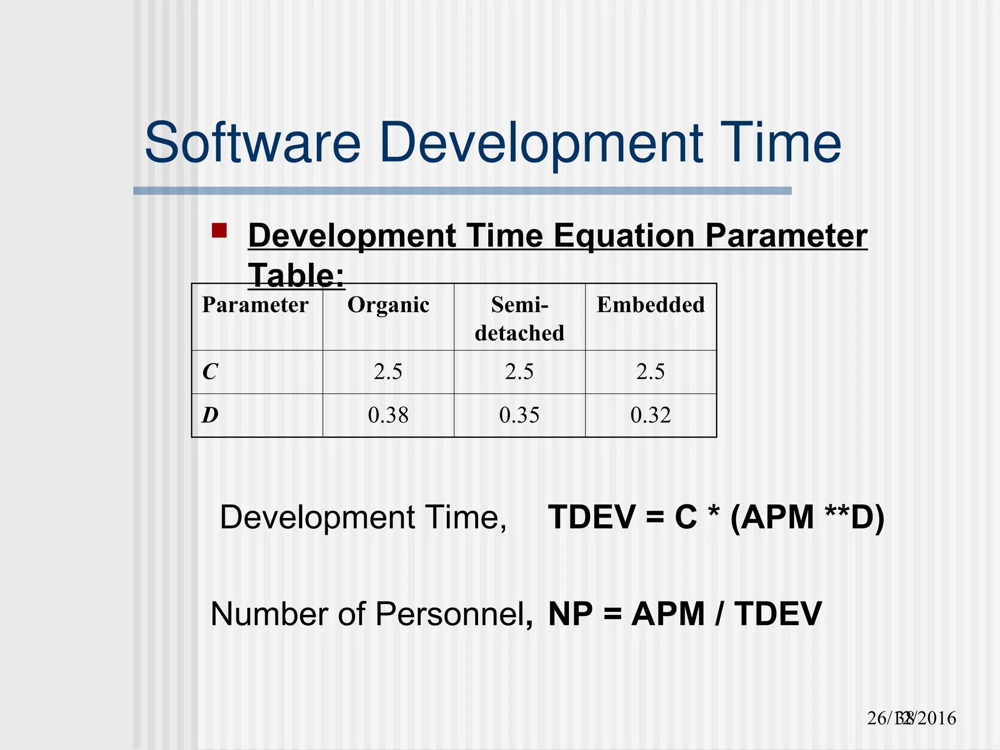
Software Development Time
 Development Time Equation Parameter
Table:
Development Time, TDEV = C * (APM **D)
Number of Personnel, NP = APM / TDEV
Parameter Organic Semi-
detached
Embedded
C 2.5 2.5 2.5
D 0.38 0.35 0.32

39. 26/12/2016
39
Distribution of Effort
 A development process typically consists of the
following stages:
 Requirements Analysis
 Design (High Level + Detailed)
 Implementation & Coding
 Testing (Unit + Integration)

40. 26/12/2016
40
Distribution of Effort (.)
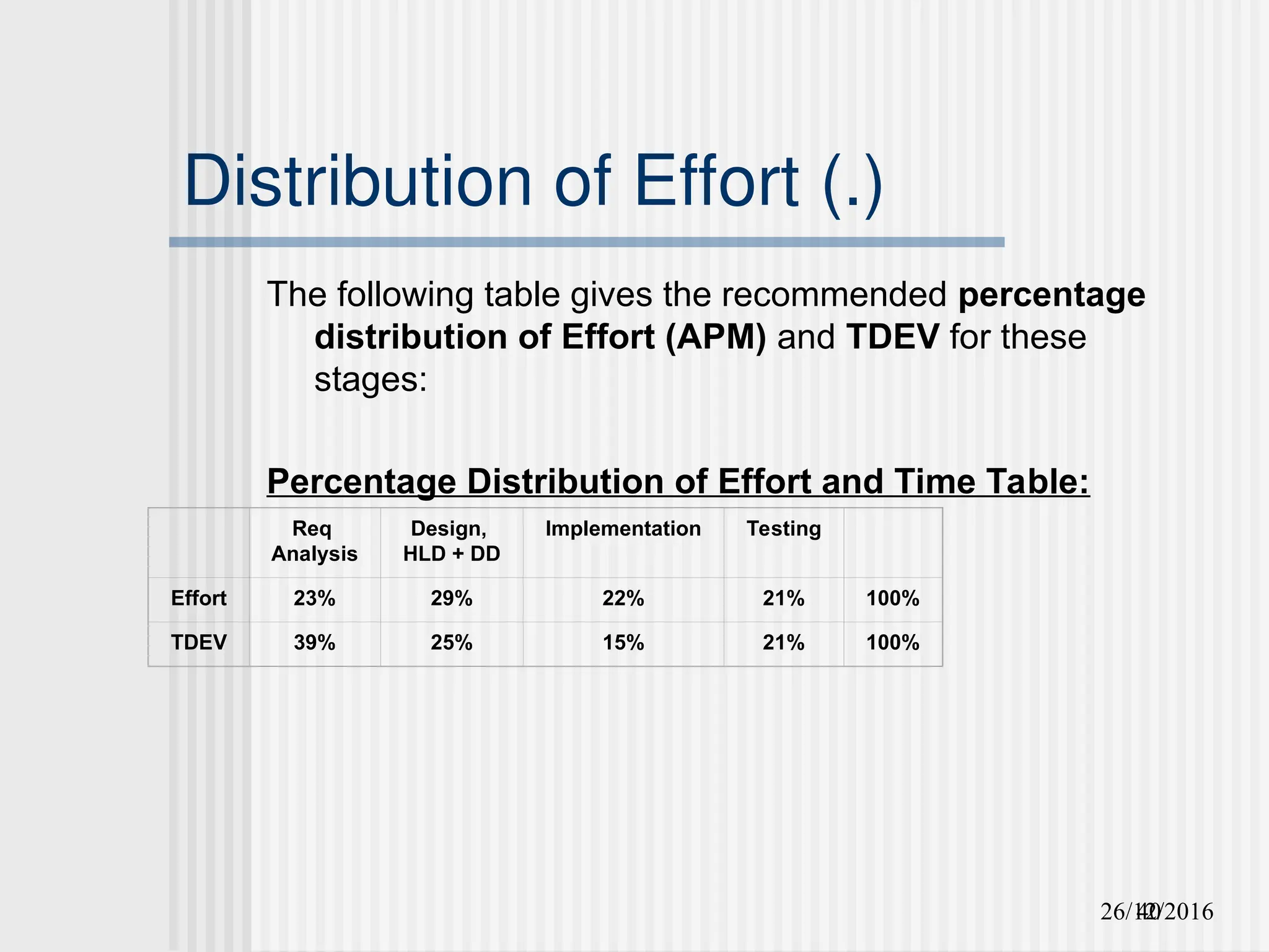
The following table gives the recommended percentage
distribution of Effort (APM) and TDEV for these
stages:
Percentage Distribution of Effort and Time Table:
Req
Analysis
Design,
HLD + DD
Implementation Testing
Effort 23% 29% 22% 21% 100%
TDEV 39% 25% 15% 21% 100%

41. 26/12/2016
41
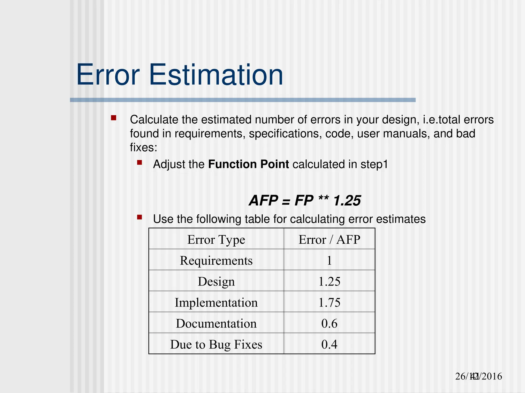
Error Estimation
 Calculate the estimated number of errors in your design, i.e.total errors
found in requirements, specifications, code, user manuals, and bad
fixes:
 Adjust the Function Point calculated in step1
AFP = FP ** 1.25
 Use the following table for calculating error estimates
Error Type Error / AFP
Requirements 1
Design 1.25
Implementation 1.75
Documentation 0.6
Due to Bug Fixes 0.4

42. 42
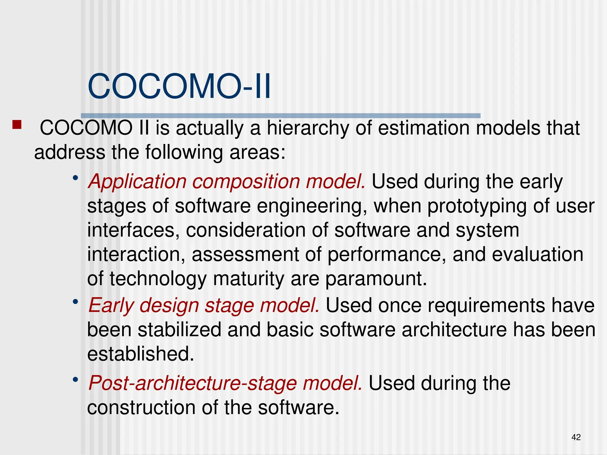
COCOMO-II
 COCOMO II is actually a hierarchy of estimation models that
address the following areas:
• Application composition model. Used during the early
stages of software engineering, when prototyping of user
interfaces, consideration of software and system
interaction, assessment of performance, and evaluation
of technology maturity are paramount.
• Early design stage model. Used once requirements have
been stabilized and basic software architecture has been
established.
• Post-architecture-stage model. Used during the
construction of the software.

43. 43
These slides are designed to accompany Software Engineering: A Practitioner’s Approach, 8/e
(McGraw-Hill 2014). Slides copyright 2014 by Roger Pressman.
The Software Equation
A dynamic multivariable model
A dynamic multivariable model
E = [LOC x B
E = [LOC x B0.333
0.333
/P]
/P]3
3
x (1/t
x (1/t4
4
)
)
where
where
E = effort in person-months or person-years
E = effort in person-months or person-years
t = project duration in months or years
t = project duration in months or years
B = “special skills factor”
B = “special skills factor”
P = “productivity parameter”
P = “productivity parameter”

44. 44
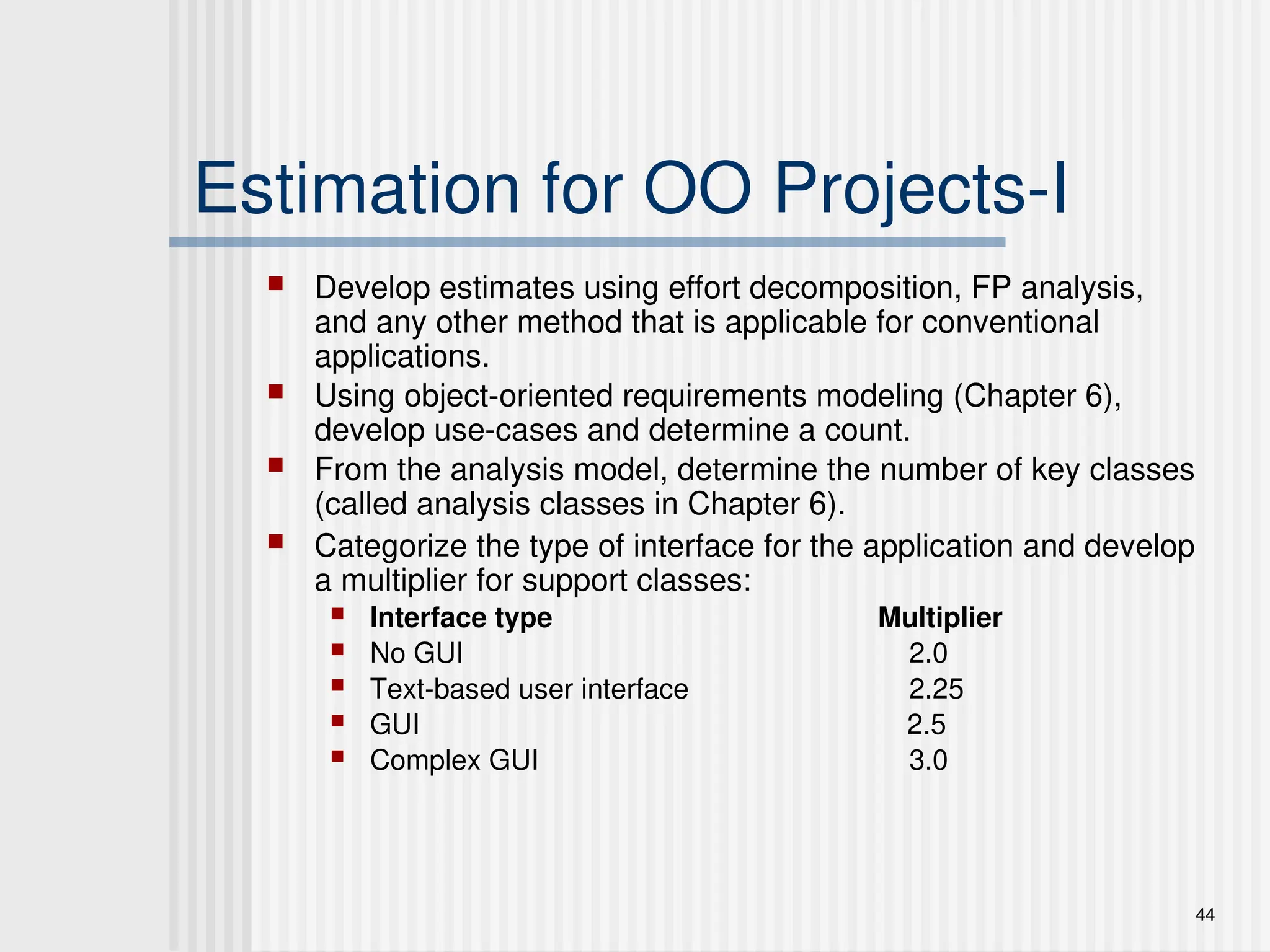
Estimation for OO Projects-I
 Develop estimates using effort decomposition, FP analysis,
and any other method that is applicable for conventional
applications.
 Using object-oriented requirements modeling (Chapter 6),
develop use-cases and determine a count.
 From the analysis model, determine the number of key classes
(called analysis classes in Chapter 6).
 Categorize the type of interface for the application and develop
a multiplier for support classes:
 Interface type Multiplier
 No GUI 2.0
 Text-based user interface 2.25
 GUI 2.5
 Complex GUI 3.0

45. 45
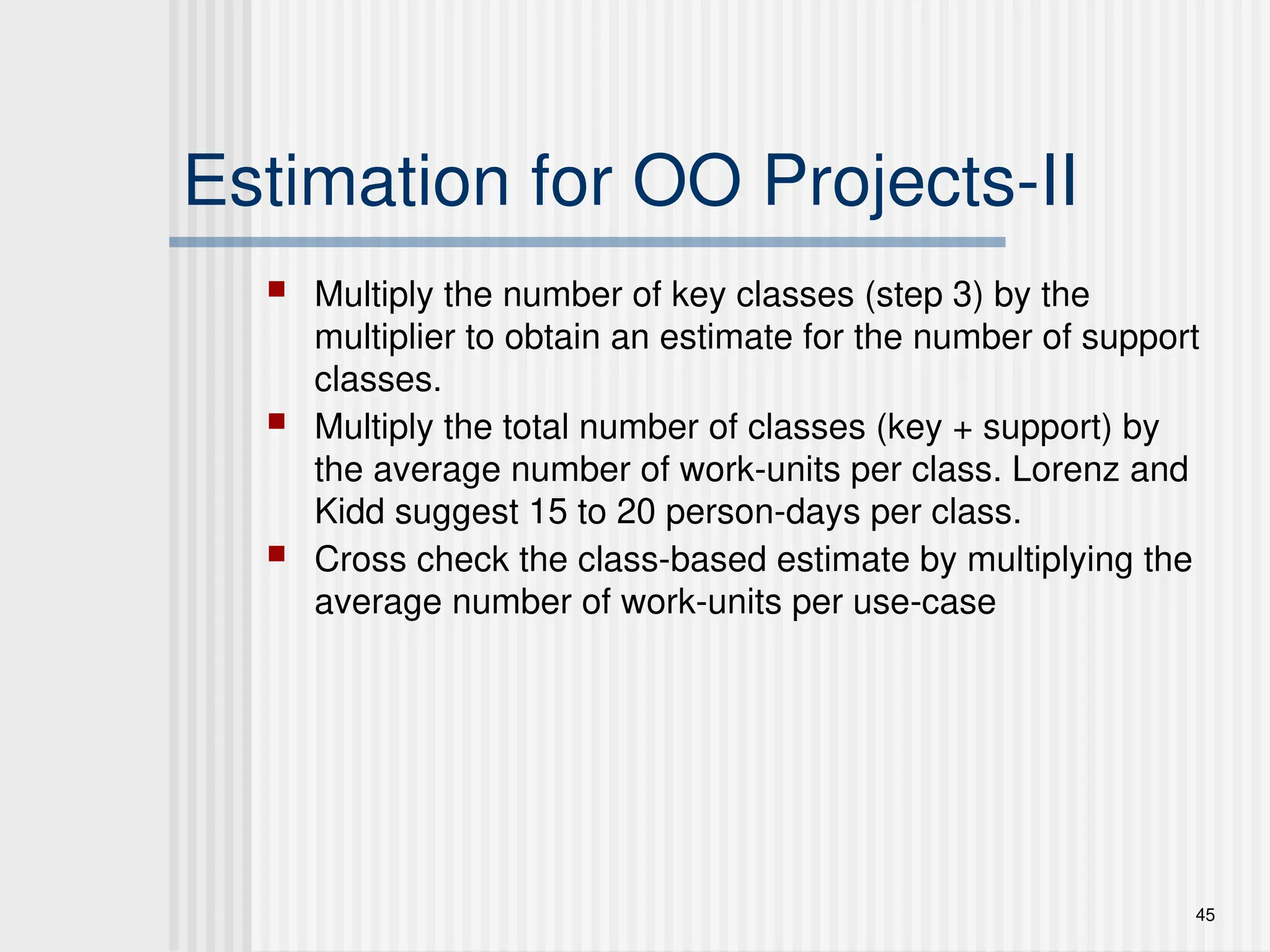
Estimation for OO Projects-II
 Multiply the number of key classes (step 3) by the
multiplier to obtain an estimate for the number of support
classes.
 Multiply the total number of classes (key + support) by
the average number of work-units per class. Lorenz and
Kidd suggest 15 to 20 person-days per class.
 Cross check the class-based estimate by multiplying the
average number of work-units per use-case

46. 46
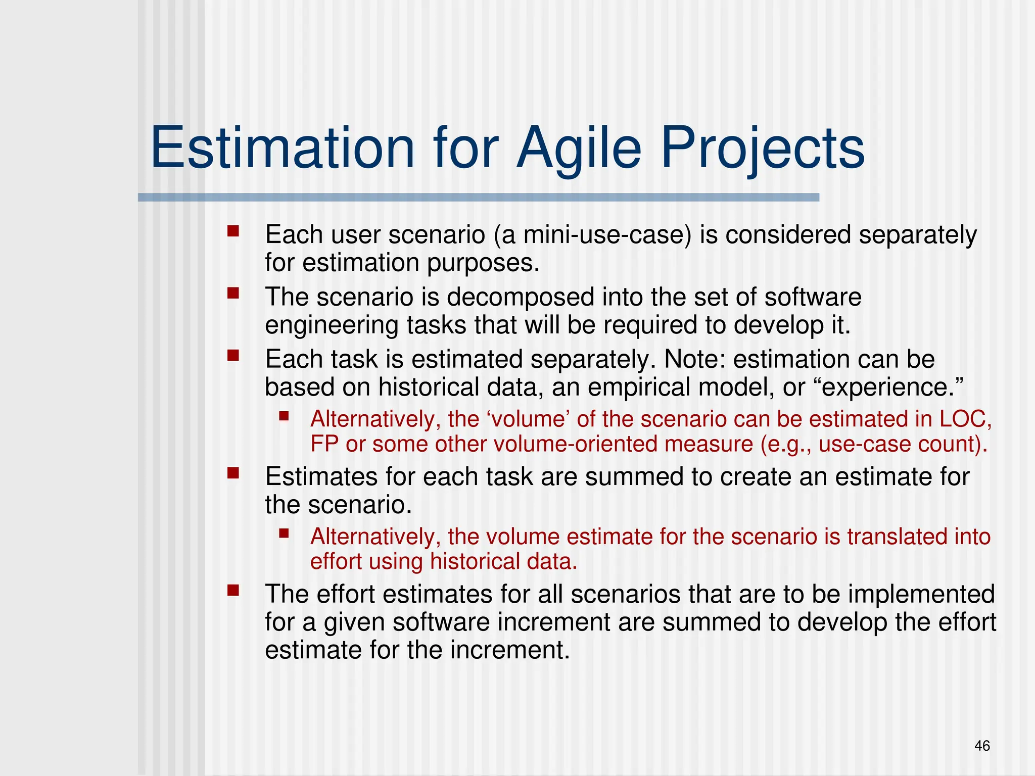
Estimation for Agile Projects
 Each user scenario (a mini-use-case) is considered separately
for estimation purposes.
 The scenario is decomposed into the set of software
engineering tasks that will be required to develop it.
 Each task is estimated separately. Note: estimation can be
based on historical data, an empirical model, or “experience.”
 Alternatively, the ‘volume’ of the scenario can be estimated in LOC,
FP or some other volume-oriented measure (e.g., use-case count).
 Estimates for each task are summed to create an estimate for
the scenario.
 Alternatively, the volume estimate for the scenario is translated into
effort using historical data.
 The effort estimates for all scenarios that are to be implemented
for a given software increment are summed to develop the effort
estimate for the increment.

47. 47
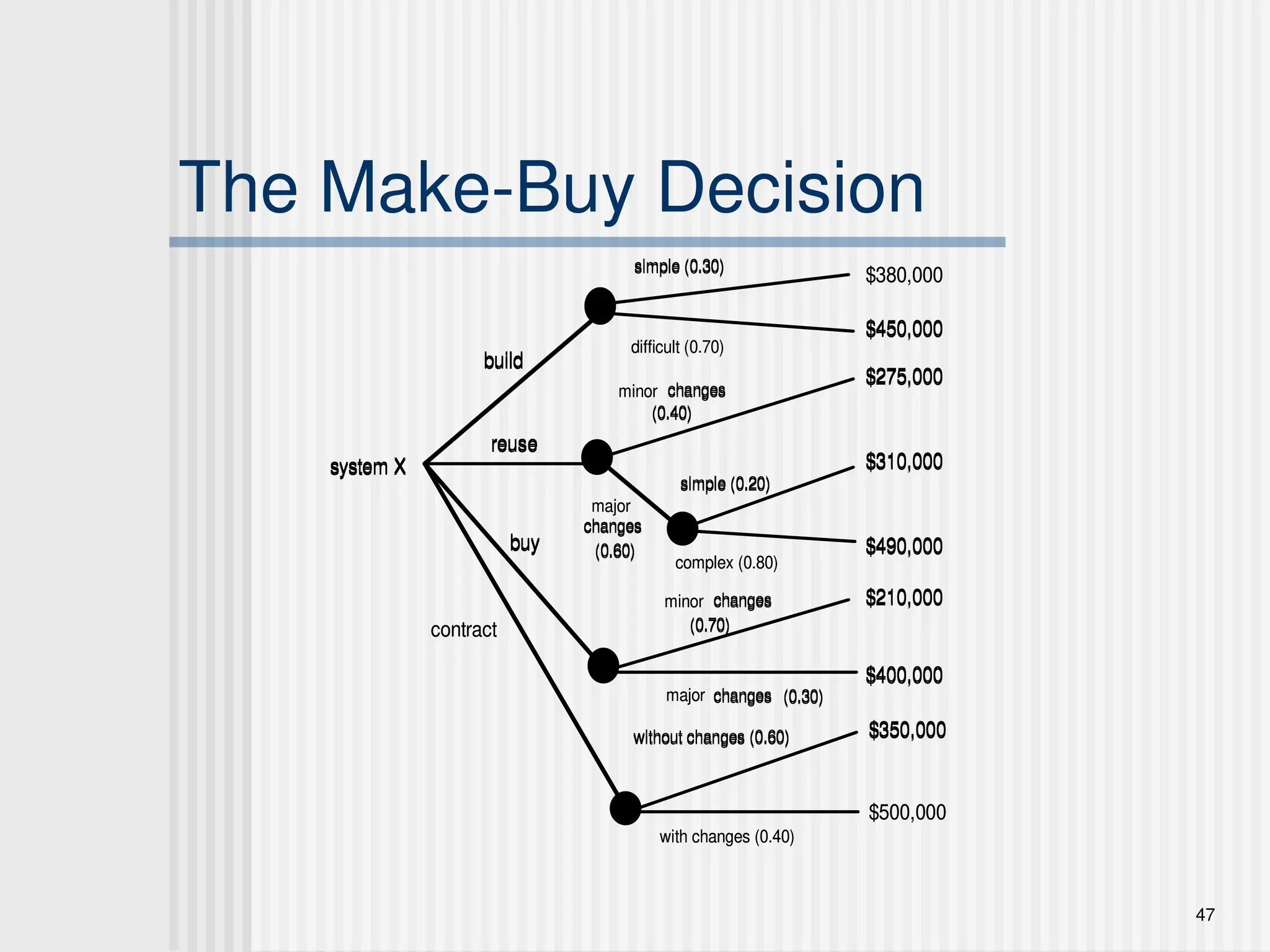
The Make-Buy Decision
system X
system X
reuse
reuse
simple (0.30)
simple (0.30)
difficult (0.70)
difficult (0.70)
minor
minor changes
changes
(0.40)
(0.40)
major
major
changes
changes
(0.60)
(0.60)
simple (0.20)
simple (0.20)
complex (0.80)
complex (0.80)
major
major changes
changes (0.30)
(0.30)
minor
minor changes
changes
(0.70)
(0.70)
$380,000
$380,000
$450,000
$450,000
$275,000
$275,000
$310,000
$310,000
$490,000
$490,000
$210,000
$210,000
$400,000
$400,000
buy
buy
contract
contract
without changes (0.60)
without changes (0.60)
with changes (0.40)
with changes (0.40)
$350,000
$350,000
$500,000
$500,000
build
build

48. 48
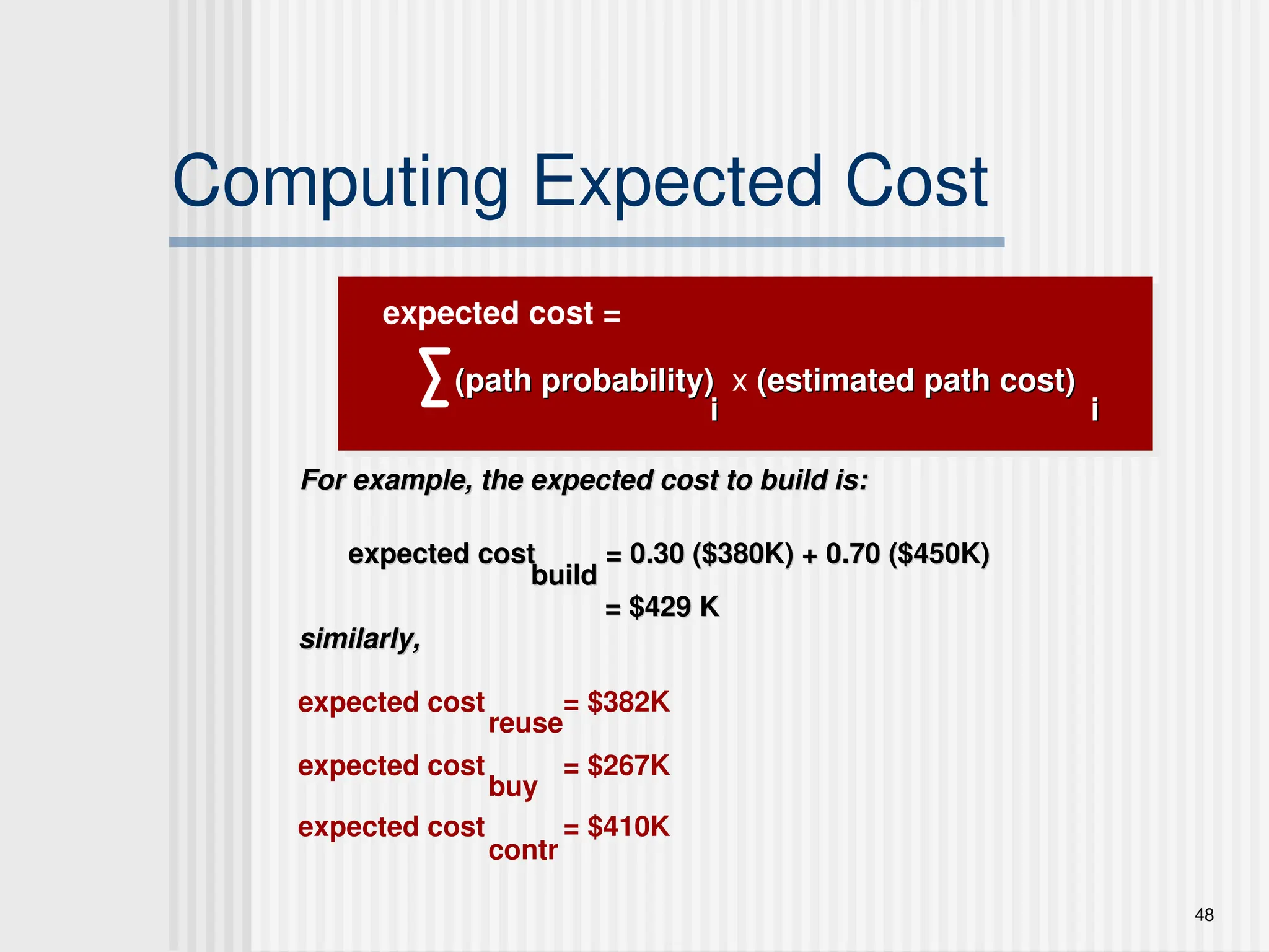
Computing Expected Cost
(path probability)
(path probability) x (estimated path cost)
(estimated path cost)
i
i i
i
For example, the expected cost to build is:
For example, the expected cost to build is:
expected cost = 0.30 ($380K) + 0.70 ($450K)
expected cost = 0.30 ($380K) + 0.70 ($450K)
similarly,
similarly,
expected cost = $382K
expected cost = $267K
expected cost = $410K
build
build
reuse
buy
contr
expected cost =
= $429 K
= $429 K

49. 49
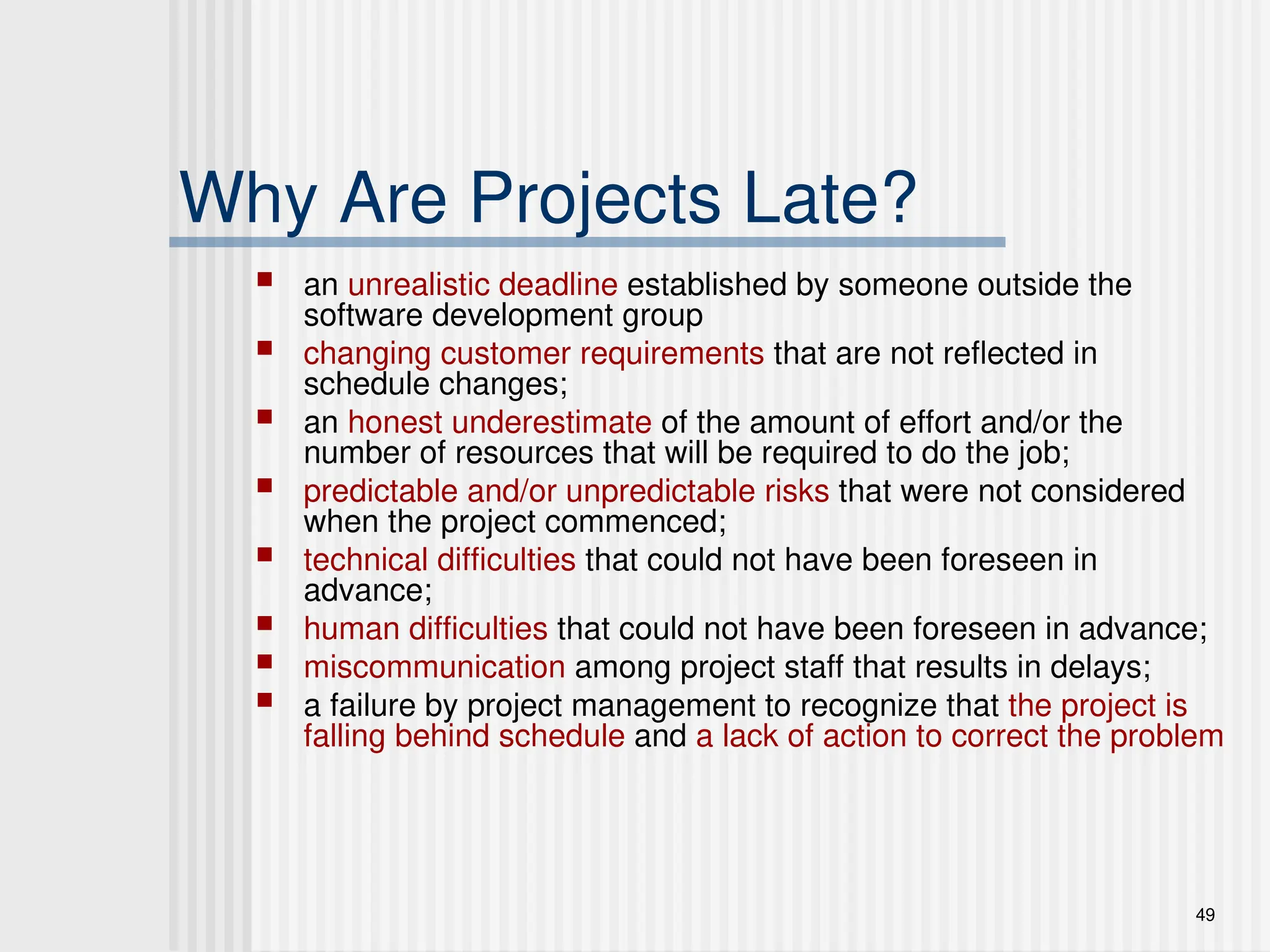
Why Are Projects Late?
 an unrealistic deadline established by someone outside the
software development group
 changing customer requirements that are not reflected in
schedule changes;
 an honest underestimate of the amount of effort and/or the
number of resources that will be required to do the job;
 predictable and/or unpredictable risks that were not considered
when the project commenced;
 technical difficulties that could not have been foreseen in
advance;
 human difficulties that could not have been foreseen in advance;
 miscommunication among project staff that results in delays;
 a failure by project management to recognize that the project is
falling behind schedule and a lack of action to correct the problem

50. Project Scheduling
50

51. 51
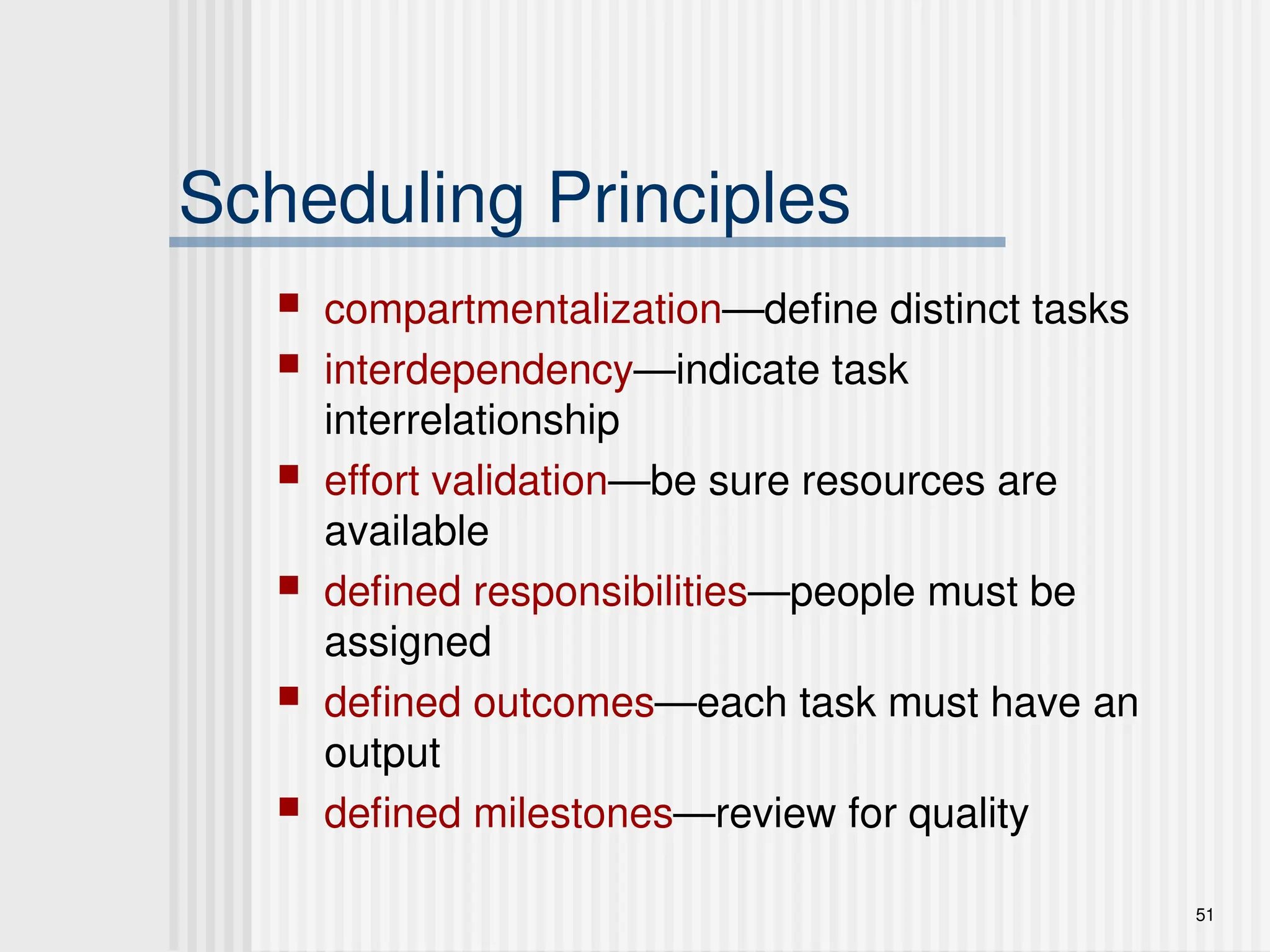
Scheduling Principles
 compartmentalization—define distinct tasks
 interdependency—indicate task
interrelationship
 effort validation—be sure resources are
available
 defined responsibilities—people must be
assigned
 defined outcomes—each task must have an
output
 defined milestones—review for quality

52. 52
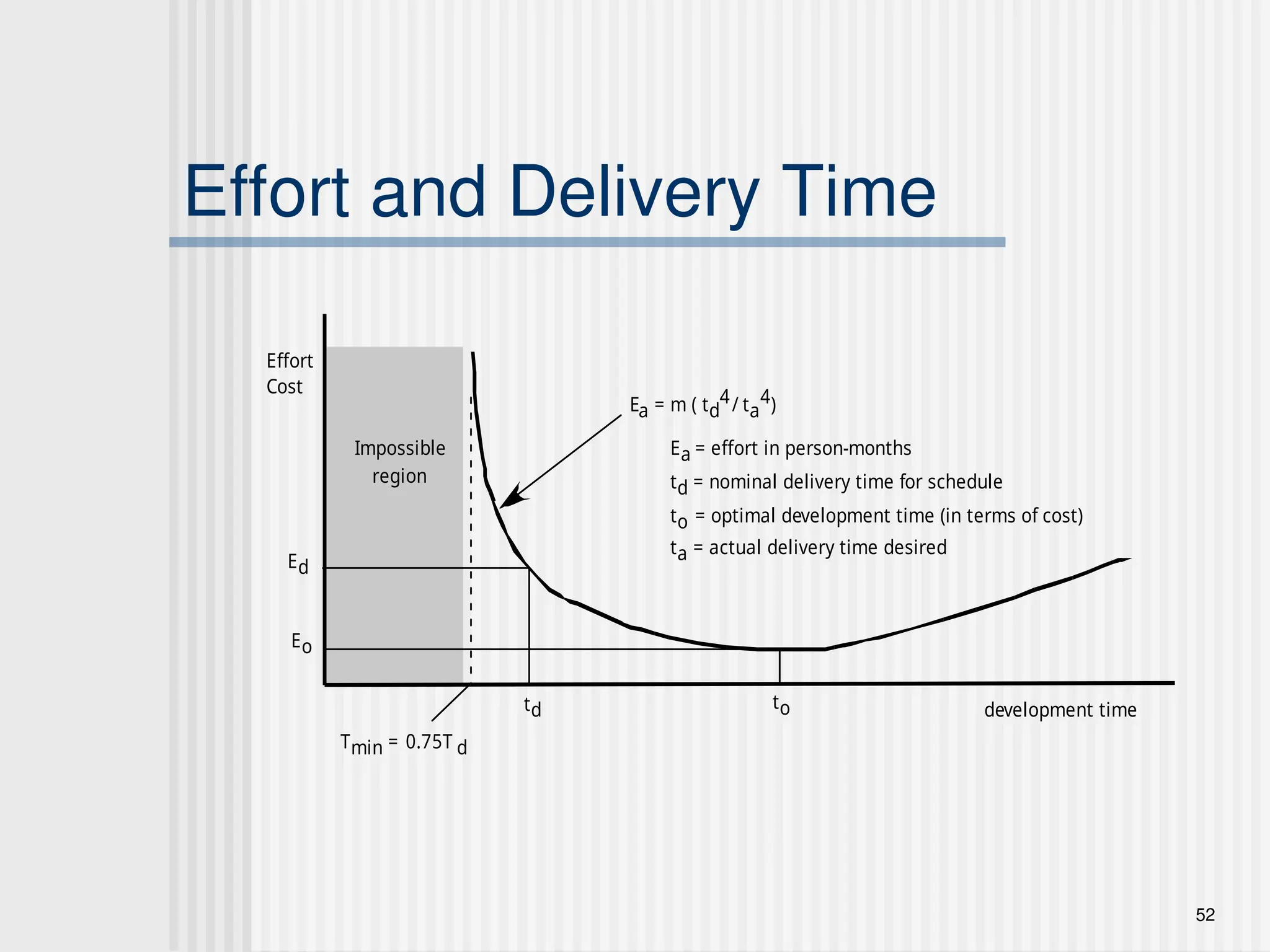
Effort and Delivery Time
Effort
Cost
Impossible
region
td
Ed
Tmin = 0.75T d
to
Eo
Ea = m ( td
4/ ta
4)
development time
Ea = effort in person-months
td = nominal delivery time for schedule
to = optimal development time (in terms of cost)
ta = actual delivery time desired

53. 53
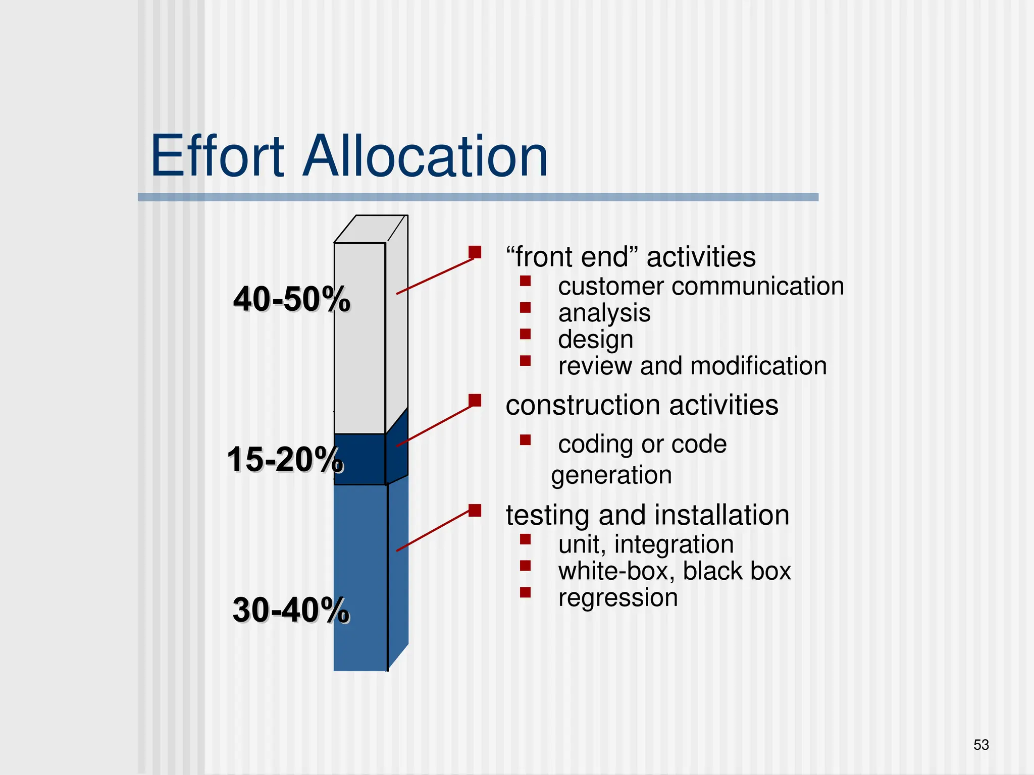
Effort Allocation
 “front end” activities
 customer communication
 analysis
 design
 review and modification
 construction activities
 coding or code
generation
 testing and installation
 unit, integration
 white-box, black box
 regression
40-50%
40-50%
30-40%
30-40%
15-20%
15-20%

54. 54
Defining Task Sets
 determine type of project
 assess the degree of rigor required
 identify adaptation criteria
 select appropriate software engineering tasks

55. 55
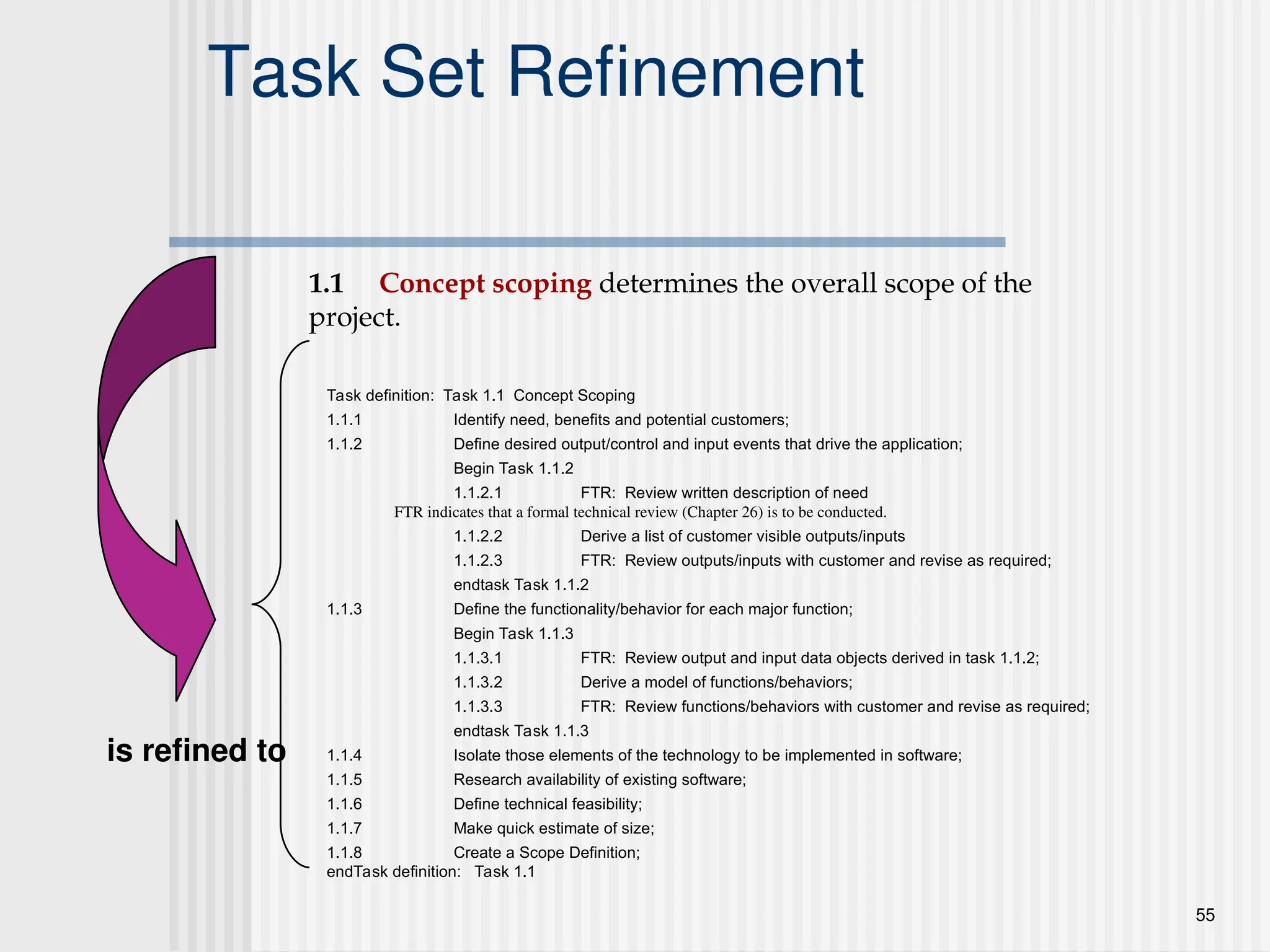
Task Set Refinement
1.1 Concept scoping determines the overall scope of the
project.
Task definition: Task 1.1 Concept Scoping
1.1.1 Identify need, benefits and potential customers;
1.1.2 Define desired output/control and input events that drive the application;
Begin Task 1.1.2
1.1.2.1 FTR: Review written description of need
FTR indicates that a formal technical review (Chapter 26) is to be conducted.
1.1.2.2 Derive a list of customer visible outputs/inputs
1.1.2.3 FTR: Review outputs/inputs with customer and revise as required;
endtask Task 1.1.2
1.1.3 Define the functionality/behavior for each major function;
Begin Task 1.1.3
1.1.3.1 FTR: Review output and input data objects derived in task 1.1.2;
1.1.3.2 Derive a model of functions/behaviors;
1.1.3.3 FTR: Review functions/behaviors with customer and revise as required;
endtask Task 1.1.3
1.1.4 Isolate those elements of the technology to be implemented in software;
1.1.5 Research availability of existing software;
1.1.6 Define technical feasibility;
1.1.7 Make quick estimate of size;
1.1.8 Create a Scope Definition;
endTask definition: Task 1.1
is refined to

56. 56
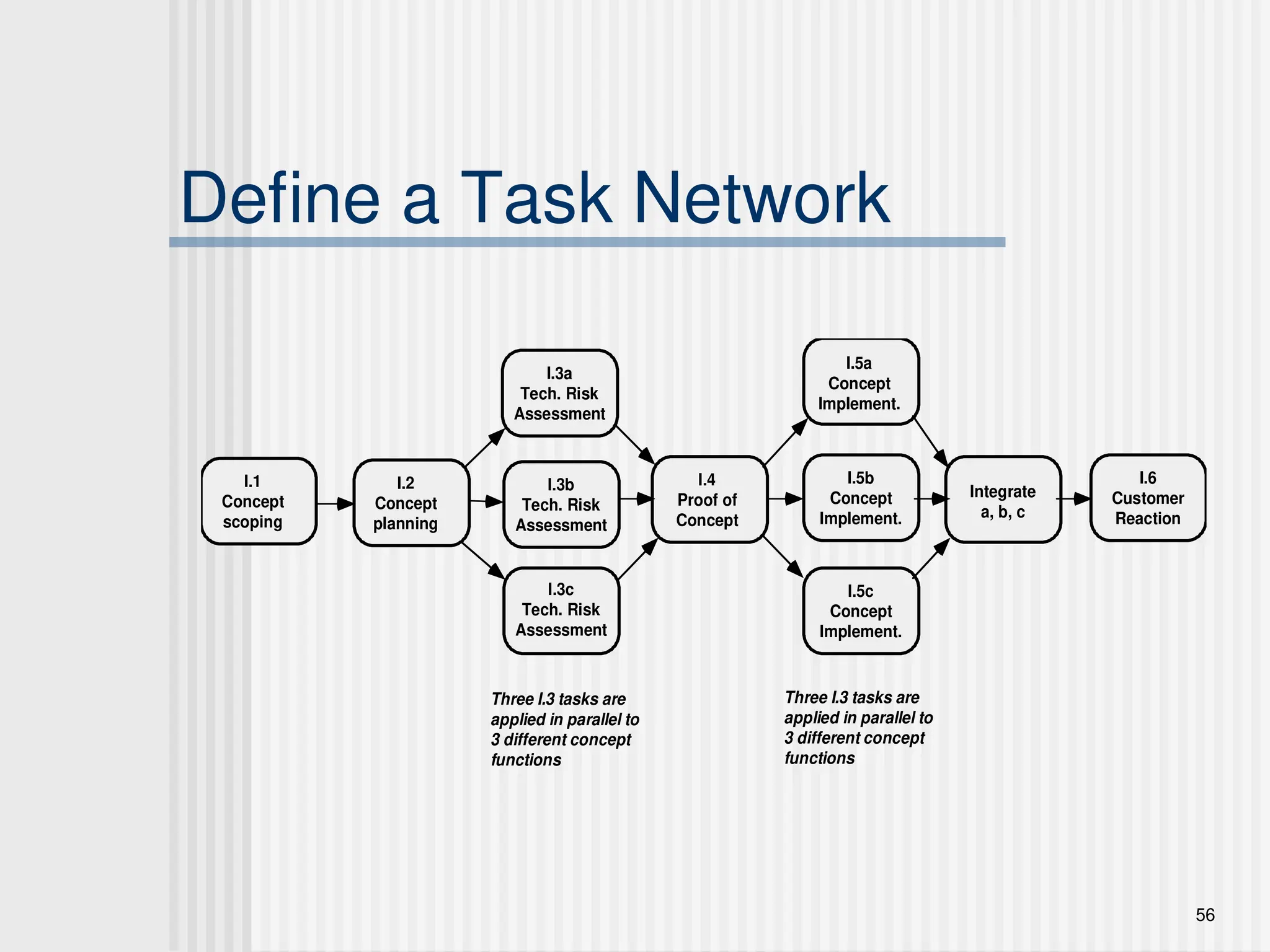
Define a Task Network
I.1
Concept
scoping
I.3a
Tech. Risk
Assessment
I.3b
Tech. Risk
Assessment
I.3c
Tech. Risk
Assessment
Three I.3 tasks are
applied in parallel to
3 different concept
functions
Three I.3 tasks are
applied in parallel to
3 different concept
functions
I.4
Proof of
Concept
I.5a
Concept
Implement.
I.5b
Concept
Implement.
I.5c
Concept
Implement.
I.2
Concept
planning
I.6
Customer
Reaction
Integrate
a, b, c

57. 57
Timeline Charts
Tasks Week 1 Week 2 Week 3 Week 4 Week n
Task 1
Task 2
Task 3
Task
4
Task 5
Task 6
Task 7
Task 8
Task 9
Task 10
Task
11
Task 12

58. 58
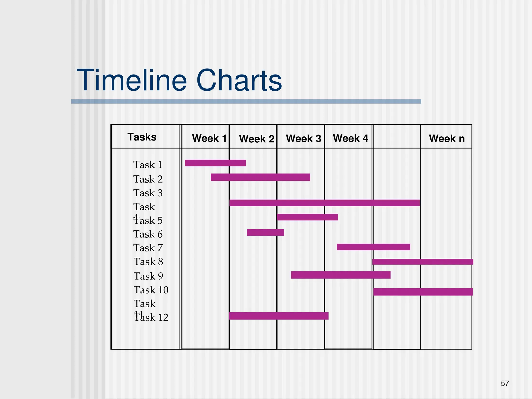
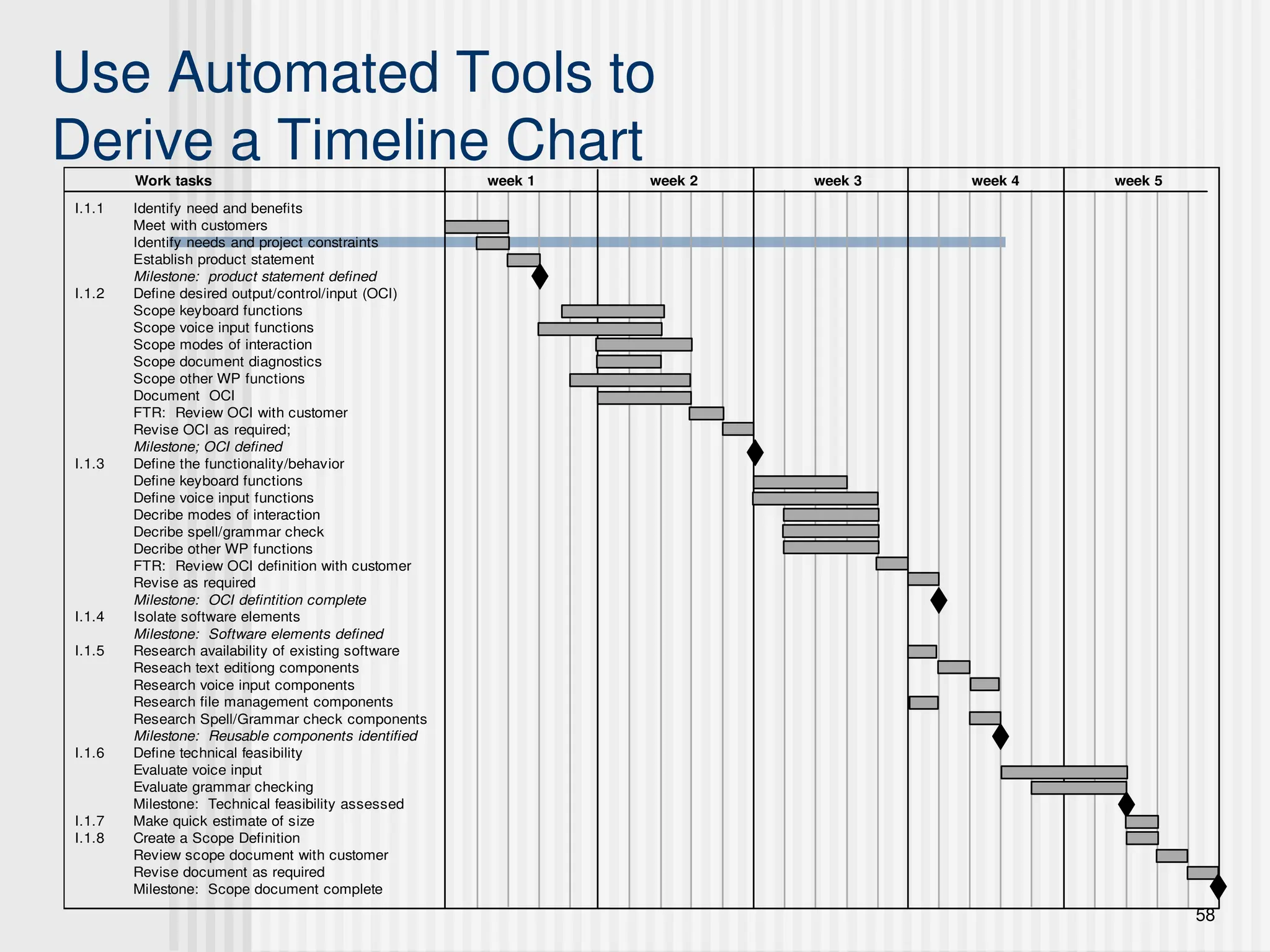
Use Automated Tools to
Derive a Timeline Chart
I.1.1 Identify need and benefits
Meet with customers
Identify needs and project constraints
Establish product statement
Milestone: product statement defined
I.1.2 Define desired output/control/input (OCI)
Scope keyboard functions
Scope voice input functions
Scope modes of interaction
Scope document diagnostics
Scope other WP functions
Document OCI
FTR: Review OCI with customer
Revise OCI as required;
Milestone; OCI defined
I.1.3 Define the functionality/behavior
Define keyboard functions
Define voice input functions
Decribe modes of interaction
Decribe spell/grammar check
Decribe other WP functions
FTR: Review OCI definition with customer
Revise as required
Milestone: OCI defintition complete
I.1.4 Isolate software elements
Milestone: Software elements defined
I.1.5 Research availability of existing software
Reseach text editiong components
Research voice input components
Research file management components
Research Spell/Grammar check components
Milestone: Reusable components identified
I.1.6 Define technical feasibility
Evaluate voice input
Evaluate grammar checking
Milestone: Technical feasibility assessed
I.1.7 Make quick estimate of size
I.1.8 Create a Scope Definition
Review scope document with customer
Revise document as required
Milestone: Scope document complete
week 1 week 2 week 3 week 4
Work tasks week 5

59. 59
Schedule Tracking
 conduct periodic project status meetings in which
each team member reports progress and problems.
 evaluate the results of all reviews conducted
throughout the software engineering process.
 determine whether formal project milestones (the
diamonds shown in Figure 34.3) have been
accomplished by the scheduled date.
 compare actual start-date to planned start-date for
each project task listed in the resource table (Figure
34.4).
 meet informally with practitioners to obtain their
subjective assessment of progress to date and
problems on the horizon.
 use earned value analysis (Section 34.6) to assess
progress quantitatively.

60. 60
Progress on an OO Project-I
 Technical milestone: OO analysis completed
• All classes and the class hierarchy have been defined and reviewed.
• Class attributes and operations associated with a class have been
defined and reviewed.
• Class relationships (Chapter 10) have been established and reviewed.
• A behavioral model (Chapter 11) has been created and reviewed.
• Reusable classes have been noted.
 Technical milestone: OO design completed
• The set of subsystems (Chapter 12) has been defined and reviewed.
• Classes are allocated to subsystems and reviewed.
• Task allocation has been established and reviewed.
• Responsibilities and collaborations (Chapter 12) have been identified.
• Attributes and operations have been designed and reviewed.
• The communication model has been created and reviewed.

61. 61
Progress on an OO Project-II
 Technical milestone: OO programming completed
• Each new class has been implemented in code from the
design model.
• Extracted classes (from a reuse library) have been
implemented.
• Prototype or increment has been built.
 Technical milestone: OO testing
• The correctness and completeness of OO analysis and design
models has been reviewed.
• A class-responsibility-collaboration network (Chapter 10) has
been developed and reviewed.
• Test cases are designed and class-level tests (Chapter 24)
have been conducted for each class.
• Test cases are designed and cluster testing (Chapter 24) is
completed and the classes are integrated.
• System level tests have been completed.

62. 62
Earned Value Analysis (EVA)
 Earned value
 is a measure of progress
 enables us to assess the “percent of completeness”
of a project using quantitative analysis rather than
rely on a gut feeling
 “provides accurate and reliable readings of
performance from as early as 15 percent into the
project.” [Fle98]

63. 63
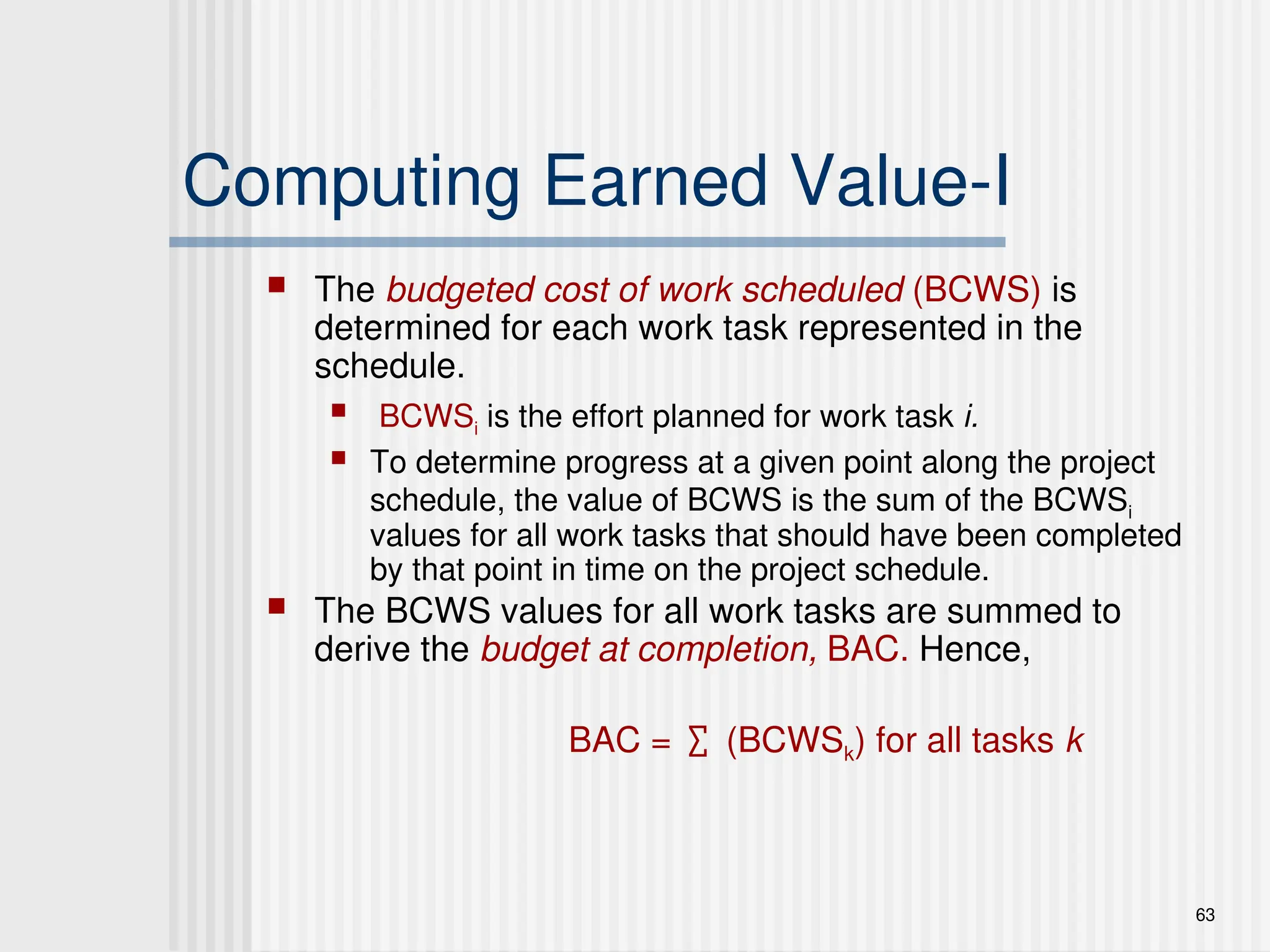
Computing Earned Value-I
 The budgeted cost of work scheduled (BCWS) is
determined for each work task represented in the
schedule.
 BCWSi is the effort planned for work task i.
 To determine progress at a given point along the project
schedule, the value of BCWS is the sum of the BCWSi
values for all work tasks that should have been completed
by that point in time on the project schedule.
 The BCWS values for all work tasks are summed to
derive the budget at completion, BAC. Hence,
BAC = ∑ (BCWSk) for all tasks k

64. 64
Computing Earned Value-II
 Next, the value for budgeted cost of work performed
(BCWP) is computed.
 The value for BCWP is the sum of the BCWS values for all
work tasks that have actually been completed by a point in time
on the project schedule.
 “the distinction between the BCWS and the BCWP is that
the former represents the budget of the activities that were
planned to be completed and the latter represents the
budget of the activities that actually were completed.”
[Wil99]
 Given values for BCWS, BAC, and BCWP, important
progress indicators can be computed:
• Schedule performance index, SPI = BCWP/BCWS
• Schedule variance, SV = BCWP – BCWS
• SPI is an indication of the efficiency with which the project is
utilizing scheduled resources.

65. 65
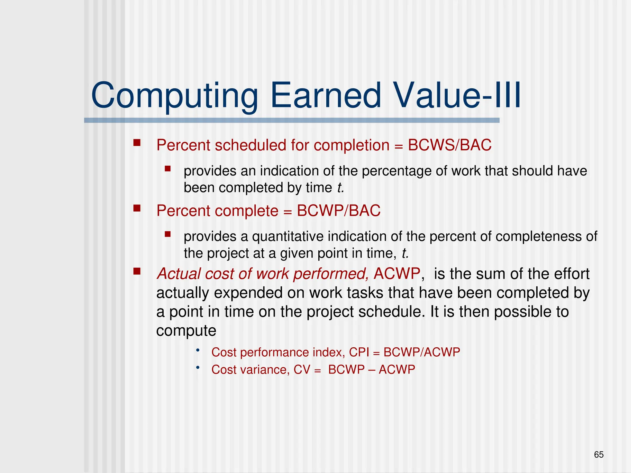
Computing Earned Value-III
 Percent scheduled for completion = BCWS/BAC
 provides an indication of the percentage of work that should have
been completed by time t.
 Percent complete = BCWP/BAC
 provides a quantitative indication of the percent of completeness of
the project at a given point in time, t.
 Actual cost of work performed, ACWP, is the sum of the effort
actually expended on work tasks that have been completed by
a point in time on the project schedule. It is then possible to
compute
• Cost performance index, CPI = BCWP/ACWP
• Cost variance, CV = BCWP – ACWP