The document provides an overview of sine sweep vibration testing, detailing its purpose in identifying natural frequencies, damping ratios, and component defects, particularly in spacecraft as used by NASA. It discusses the characteristics of sine sweep tests, including frequency variations, amplitude metrics, and the use of logarithmic sweep rates. Additionally, the document outlines practical applications, examples, and exercises related to sine sweep testing in solid rocket motors and single degree of freedom systems.

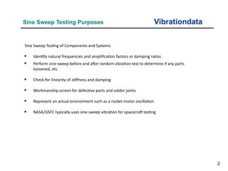
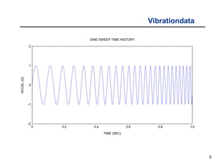
1. 1
Sine Sweep Vibration
Vibrationdata
Unit 3

2. 2
Vibrationdata
Sine Sweep Testing Purposes
Sine Sweep Testing of Components and Systems

Identify natural frequencies and amplification factors or damping ratios

Perform sine sweep before and after random vibration test to determine if any parts
loosened, etc.

Check for linearity of stiffness and damping

Workmanship screen for defective parts and solder joints

Represent an actual environment such as a rocket motor oscillation

NASA/GSFC typically uses sine sweep vibration for spacecraft testing

3. 3
Vibrationdata
-2
-1
1
2
0
0 0.2 0.4 0.6 0.8 1.0
TIME (SEC)
ACCEL
(G)
SINE SWEEP TIME HISTORY

4. 4
Vibrationdata
Sine Sweep Characteristics
• The essence of a sine sweep test is that the base excitation input consists of a
single frequency at any given time.
• The frequency itself, however, is varied with time.
• The sine sweep test may begin at a low frequency and then sweep to a high
frequency, or vice-versa.
• Some specifications require several cycles, where one cycle is defined as from low
to high frequency and then from high back to low frequency.

5. 5
Vibrationdata
Sine Sweep Rate
• The specification might require either a linear or a logarithmic sweep rate.
• The sweep will spend greater time at the lower frequency end if the
sweep is logarithmic.
• The example in the previous figure had a logarithmic sweep rate.
• The amplitude in the previous is constant.
• Nevertheless, the specification might require that the amplitude vary with
frequency.

6. 6
Vibrationdata
Sine Sweep Specification Example
• A vendor has a product that must withstand sinusoidal vibration with an
amplitude of 12 G.
• The desired frequency domain is 10 Hz to 2000 Hz.
• The shaker table has a displacement limit of 1.0 inch peak-to-peak, or 0.5
inch zero-to-peak.
• Recall that the displacement limit is a constraint at low frequencies.
• How should the test be specified?
• The answer is to use a specification with two amplitude segments.
• The first segment is a constant displacement ramp.
• The second segment is a constant acceleration plateau.

7. 7
Vibrationdata
Sine Amplitude Metrics
Ramp is 1.0 inch peak-peak. Plateau is 12 G.

8. 8
Vibrationdata
Crossover Frequency
8
The "crossover" frequency is 15.3 Hz. This is the frequency at which a 12 G acceleration
has a corresponding displacement of 1.0 inch peak-to-peak. The crossover frequency
fcross is calculated via
Furthermore, the acceleration should be converted from G to in/sec2
or G to m/sec2
, as
appropriate.

9. 9
Vibrationdata
Octaves
• One octave is defined as a frequency band where the upper frequency limit is equal to
twice the lower frequency limit.
• Thus a band from 10 Hz to 20 Hz is one octave.
• Likewise, the band from 20 Hz to 40 Hz is an octave.
• A concern regarding sine sweep testing is the total number of octaves.
• As an example consider the following frequency sequence in Hertz.
10 - 20 - 40 - 80 -160 - 320 - 640 - 1280 – 2560
• The sequence has a total of eight octaves.

10. 10
Vibrationdata
Octave Formulas
where f1 and f2 are the lower and upper frequency limits, respectively.
Thus, the frequency domain from 10 Hz to 2000 Hz has 7.64 octaves
• Now consider a sine sweep test from 10 Hz to 2000 Hz.
• How many octaves are in this example?
• A rough estimate is 7.5.
• Nevertheless, the exact number is needed.
• The number of octaves n can be calculated in terms of natural logarithms as

11. 11
Vibrationdata
Rate & Duration
• The number of octaves is then used to set the sweep rate, assuming a logarithmic rate.
• For example, the rate might be specified as 1 octave/minute.
• The duration for 7.64 octaves would thus be: 7 minutes 38 seconds
• The excitation frequency at any time can then be calculated from this rate.
• Or perhaps the total sweep time from 10 Hz to 2000 Hz is specified as 8 minutes.
• Thus, the sweep rate is 0.955 octaves/min.

12. 12
Vibrationdata
SDOF Response Example
Apply sine sweep base input to an SDOF system (fn=40 Hz, Q=10)
Input Specification:
10 Hz, 1 G
80 Hz, 1 G
Duration 180 seconds
3 octaves
Log sweep 1 octave/min
Synthesize time history with Matlab GUI script: vibrationdata.m
vibrationdata > Miscellanous Functions > Generate Signal > Sine Sweep

13. 13
Vibrationdata
Input Sine Sweep, Segment
Entire time history
is 180 seconds

14. 14
Vibrationdata
Input Sine Sweep, Waterfall FFT
The series of peaks forms a
curved line because the
sweep rate is logarithmic.
Waterfall FFT

15. 15
SDOF System Subjected to Base Excitation Vibrationdata
The equation of motion was previously derived in Webinar 2.
Highlights are shown on the next slide.

16. 16
Free Body Diagram Vibrationdata
Summation of forces in the vertical direction
Let z = x - y. The variable z is thus the relative displacement.
Substituting the relative displacement yields
)
x
(y
k
)
x
y
(
c
x
m 


 



y
(k/m)z
z
(c/m)
z 



 



x
m
F 



n
ω
ξ
2
c/m  2
n
ω
k/m 
y
z
2
n
ω
z
n
ω
2ξ
z 



 




17. 17
Vibrationdata
Solving the Equation of Motion
A convolution integral is used for the case where the base input acceleration is arbitrary.
The convolution integral is numerically inefficient to solve in its equivalent digital-series
form.
Instead, use…
Smallwood, ramp invariant, digital recursive filtering relationship!
Synthesize time history with Matlab GUI script: vibrationdata.m
vibrationdata > SDOF Response to Base Input

18. 18
Vibrationdata
SDOF Response

19. 19
Vibrationdata
Solid Rocket Pressure Oscillation
• Solid rocket motors may have pressure oscillations which form in the
combustion chamber
• Various vortex-shedding and other effects cause standing waves to form in the
combustion cavity
• This effect is sometimes called “Resonant Burn” or “Thrust Oscillation”
• The sinusoidal oscillation frequency may sweep downward as the cavity
volume increases due to the conversion of propellant to exhaust gas

20. 20
Vibrationdata
Solid Rocket Motor Example

21. 21
Vibrationdata
Flight Accelerometer Data

22. 22
Vibrationdata
Flight Accelerometer Data, Segment

23. 23
Vibrationdata
Time-Varying Statistics
• Calculate statistics for each consecutive 0.5-second segment
• Use Matlab GUI script: vibrationdata.m
Vibrationdata > Time-Varying Freq & Amp

24. 24
44 46 48 50 52 54 56 58 60 62 64
350
400
450
500
550
FREQUENCY
Time(sec)
Freq(Hz)

25. 25
42 44 46 48 50 52 54 56 58 60 62 64
0
0.2
0.4
0.6
0.8
1
1.2
1.4
1.6
1.8
Time (sec)
Accel(G)
peak
std dev
average

26. 26
340 360 380 400 420 440 460 480 500 520 540
0
0.2
0.4
0.6
0.8
1
1.2
1.4
1.6
1.8
PEAK vs. FREQUENCY
Peak
Accel
(G)
Freq(Hz)

27. 27
Solid Rocket Motor Flight Data – Waterfall FFT
Waterfall FFTs will be covered in a future webinar

28. 28
Vibrationdata
Exercise 1

A shaker table has a displacement limit of 1.5 inch peak-to-peak, or 0.75 inch zero-to-peak.

An amplitude of 28 G is desired from 10 Hz to 2000 Hz.

The specification will consist of a displacement ramp and an acceleration plateau.

What should the crossover frequency be?

Use Matlab GUI script: vibrationdata.m
vibrationdata > Miscellaneous Functions > Sine Sweep Parameters > Cross-over Frequency

What is the maximum acceleration at 10 Hz?
vibrationdata > Miscellaneous Functions > Amplitude Conversion Utilities > Steady-State Sine
Amplitude

29. 29
Vibrationdata
Exercise 2
Apply sine sweep base input to an SDOF system (fn=60 Hz, Q=10)
Input Specification:
10 Hz, 1 G
80 Hz, 1 G
Duration 180 seconds, Sample Rate = 2000 Hz
3 octaves
Log sweep 1 octave/min
Synthesize time history with Matlab GUI script: vibrationdata.m
vibrationdata > Miscellanous Functions > Generate Signal > Sine Sweep
Save time history in Matlab workspace as: sine_sweep
Then calculate SDOF Response (fn=60 Hz, Q=10) to the sine sweep
vibrationdata > SDOF Response to Base Input

30. 30
Vibrationdata
Exercise 3
• Calculate statistics for each consecutive 0.5-second segment
• Use Matlab GUI script: vibrationdata.m
Vibrationdata > Time-Varying Freq & Amp
• Call in external ASCII file:
solid_motor.dat - time (sec) & accel (G)