This slide shows the new's paper seller problem to find the profit, salvage and loss

1. Lecture 8
Simulation of Queueing System
Simulation of Inventory Systems

2. Simulation of Inventory Systems (1)
This inventory system has a
periodic review of length N, at
which time the inventory level is
checked.
An order is made to bring the
inventory up to the level M.
In this inventory system the lead
time (i.e., the length of time
between the placement and
receipt of an order) is zero.
Demand is shown as being
uniform over the time period

3. Notice that in the second cycle, the amount in inventory drops below
zero, indicating a shortage.
Two way to avoid shortages
 Carrying stock in inventory
: cost - the interest paid on the funds borrowed to buy the items, renting
of storage space, hiring guards, and so on.
 Making more frequent reviews, and consequently, more frequent
purchases or replenishments
: the ordering cost
The total cost of an inventory system is the measure of performance.
 The decision maker can control the maximum inventory level, M, and the
length of the cycle, N.
 In an (M,N) inventory system, the events that may occur are: the demand
for items in the inventory, the review of the inventory position, and the
receipt of an order at the end of each review period.
Simulation of Inventory Systems (2)

4. Example 2.3 The Newspaper Seller’s Problem
 A classical inventory problem concerns the purchase and sale
of newspapers.
 The paper seller buys the papers for 33 cents each and sells
them for 50 cents each. (The lost profit from excess demand is
17 cents for each paper demanded that could not be provided.)
 Newspapers not sold at the end of the day are sold as scrap for
5 cents each. (the salvage value of scrap papers)
 Newspapers can be purchased in bundles of 10. Thus, the
paper seller can buy 50, 60, and so on.
 There are three types of newsdays, “good,” “fair,” and “poor,”
with probabilities of 0.35, 0.45, and 0.20, respectively.
2.2 Simulation of Inventory Systems (3)

5. Simulation of Inventory Systems (4)
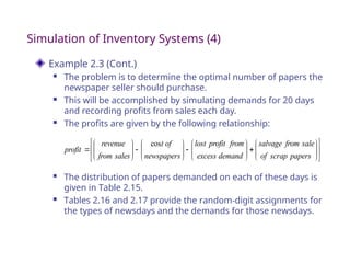
Example 2.3 (Cont.)
 The problem is to determine the optimal number of papers the
newspaper seller should purchase.
 This will be accomplished by simulating demands for 20 days
and recording profits from sales each day.
 The profits are given by the following relationship:










































papers
scrap
of
sale
from
salvage
demand
excess
from
profit
lost
newspapers
of
t
sales
from
revenue
profit
cos
 The distribution of papers demanded on each of these days is
given in Table 2.15.
 Tables 2.16 and 2.17 provide the random-digit assignments for
the types of newsdays and the demands for those newsdays.

6. Simulation of Inventory Systems (5)

7. Example 2.3 (Cont.)
 The simulation table for the decision to purchase 70 newspapers is
shown in Table 2.18.
 The profit for the first day is determined as follows:
Profit = $30.00 - $23.10 - 0 + $.50 = $7.40
 On day 1 the demand is for 60 newspapers. The revenue from the sale of 60
newspapers is $30.00.
 Ten newspapers are left over at the end of the day.
 The salvage value at 5 cents each is 50 cents.
 The profit for the 20-day period is the sum of the daily profits, $174.90. It
can also be computed from the totals for the 20 days of the simulation as
follows:
 Total profit = $645.00 - $462.00 - $13.60 + $5.50 = $174.90
 The policy (number of newspapers purchased) is changed to other values
and the simulation repeated until the best value is found.
Simulation of Inventory Systems (6)

9. Example 2.4 Simulation of an (M,N) Inventory System
 This example follows the pattern of the probabilistic order-level
inventory system shown in Figure 2.7.
 Suppose that the maximum inventory level, M, is11 units and the
review period, N, is 5 days. The problem is to estimate, by
simulation, the average ending units in inventory and the
number of days when a shortage condition occurs.
 The distribution of the number of units demanded per day is
shown in Table 2.19.
 In this example, lead time is a random variable, as shown in Table
2.20.
 Assume that orders are placed at the close of business and are
received for inventory at the beginning of business as
determined by the lead time.
Simulation of Inventory Systems (7)

10. Example 2.4 (Cont.)
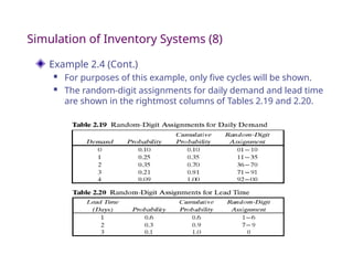
 For purposes of this example, only five cycles will be shown.
 The random-digit assignments for daily demand and lead time
are shown in the rightmost columns of Tables 2.19 and 2.20.
Simulation of Inventory Systems (8)

11. Note
Beginning inventory – Demand = Ending Inventory
If Demand is greater than Beginning Inventory than shortage
occur
Days until Order Arrives = Lead Time
Order Quantity = 11 – Ending Inventory

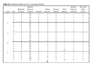
13. Example 2.4 (Cont.)
 The simulation has been started with the inventory level at 3
units and an order of 8 units scheduled to arrive in 2 days' time.
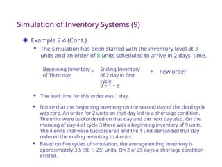
Simulation of Inventory Systems (9)
Beginning Inventory
of Third day
Ending Inventory
of 2 day in first
cycle
new order
9 = 1 + 8
= +
 Notice that the beginning inventory on the second day of the third cycle
was zero. An order for 2 units on that day led to a shortage condition.
The units were backordered on that day and the next day also. On the
morning of day 4 of cycle 3 there was a beginning inventory of 9 units.
The 4 units that were backordered and the 1 unit demanded that day
reduced the ending inventory to 4 units.
 Based on five cycles of simulation, the average ending inventory is
approximately 3.5 (88  25) units. On 2 of 25 days a shortage condition
existed.
 The lead time for this order was 1 day.