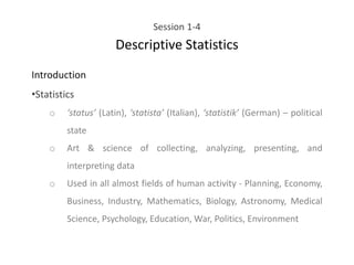
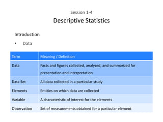
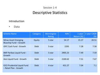
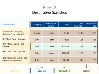
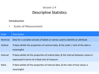
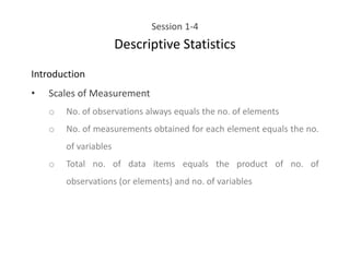
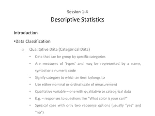
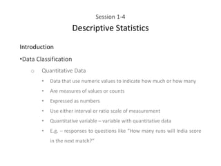
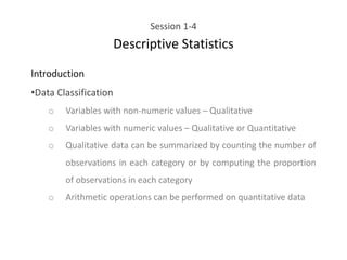
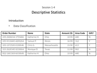
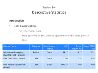
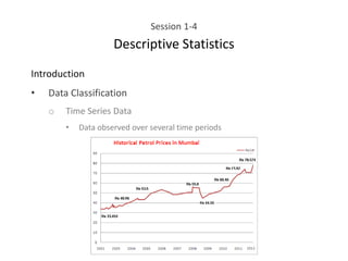
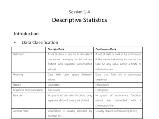
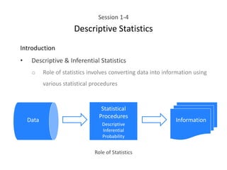
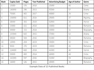
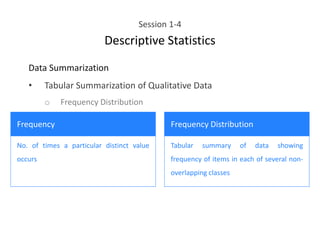
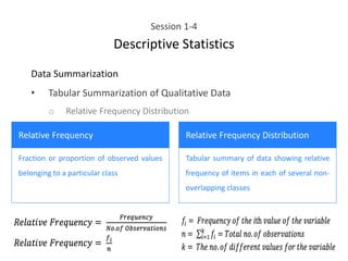
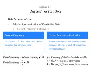
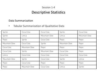
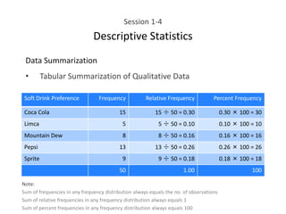
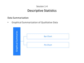
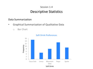
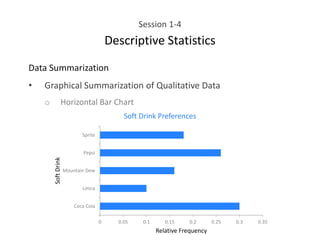
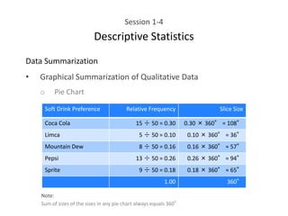
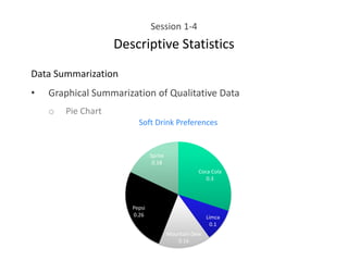
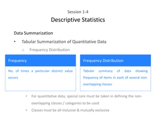
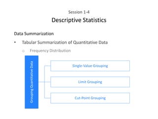
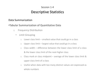
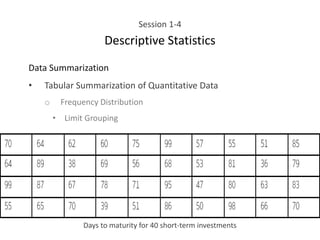
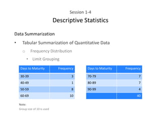
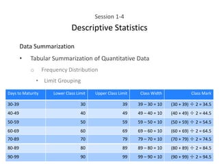
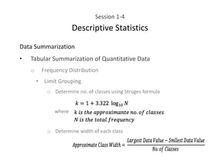
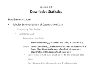
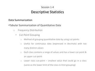
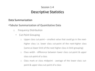
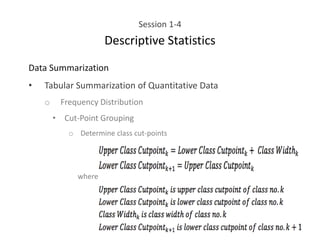
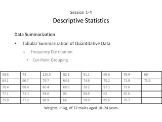
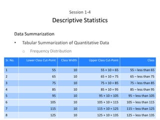
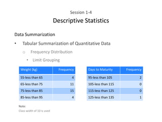
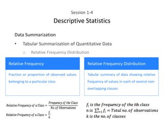
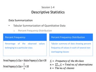
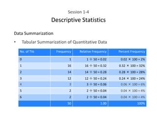
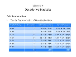
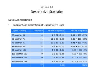
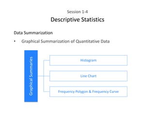
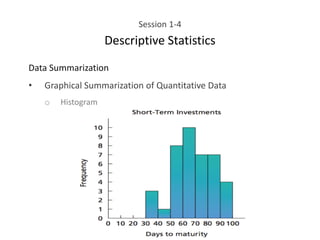
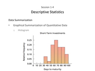
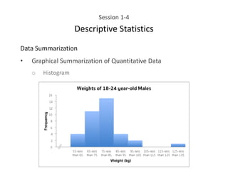
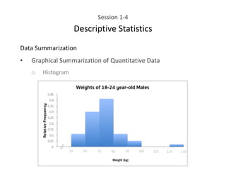
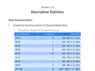
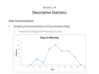
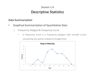
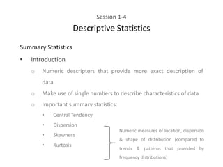
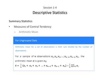
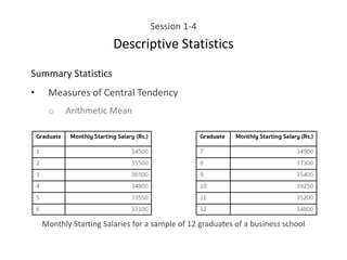
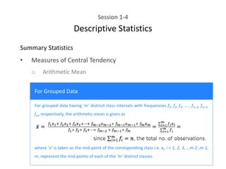
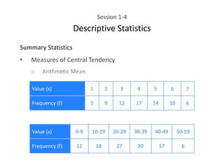
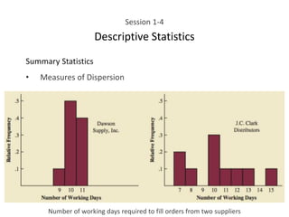
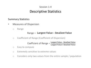
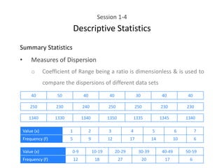
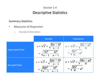
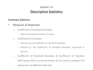
Session 1-4 - Descriptive Statistics.pdf

Session 1-4
Descriptive Statistics
• Introduction
o Statistics
o Data
o Scales of Measurement
o Data Classification
o Descriptive & Inferential Statistics
• Data Summarization
o Tabular Summarization of Qualitative Data
o Graphical Summarization of Qualitative Data

Session 1-4
o Tabular Summarization of Quantitative Data
o Graphical Summarization of Quantitative Data
• Summary Statistics
o Introduction
o Measures of Central Tendency
o Measures of Dispersion
o Measures of Skewness

Session 1-4
Introduction
•Statistics
o ‘status’ (Latin), ‘statista’ (Italian), ‘statistik’ (German) – political
state
o Art & science of collecting, analyzing, presenting, and
interpreting data
o Used in all almost fields of human activity - Planning, Economy,
Business, Industry, Mathematics, Biology, Astronomy, Medical
Science, Psychology, Education, War, Politics, Environment

Session 1-4
Introduction
• Data
Term Meaning / Definition
Data Facts and figures collected, analyzed, and summarized for
presentation and interpretation
Data Set All data collected in a particular study
Elements Entities on which data are collected
Variable A characteristic of interest for the elements
Observation Set of measurements obtained for a particular element

Session 1-4
Introduction
• Data
Scheme Name Category Morningstar
Rating
NAV 1-year
Return (%)
5-year CAGR
(%)
Mirae Asset Emerging
Bluechip Fund – Growth
Equity 5-star 54.17 15.17 20.51
IDFC Cash Fund - Growth Debt 5-star 2295 7.28 7.58
BNP Paribas Liquid Fund -
Growth
Debt 5-star 2905.23 7.49 7.59
Axis Liquid Fund - Growth Debt 5-star 2100.62 7.51 7.67
ICICI Prudential Liquid Fund
– Retail Plan - Growth
Debt 4-star 431.27 7.04 7.1

Category
Morningstar
Rating
NAV
1-year
Return (%)
5-year CAGR
(%)
Equity 5-star 54.17 15.17 20.51
Debt 5-star 2295 7.28 7.58
Debt 5-star 2905.23 7.49 7.59
Debt 5-star 2100.62 7.51 7.67
Debt 4-star 431.27 7.04 7.1
IDFC Cash Fund - Growth
Growth
Axis Liquid Fund - Growth
ICICI Prudential Liquid Fund
– Retail Plan - Growth
Scheme Name
Elements Variables Data Set
Observation
Session 1-4

Session 1-4
Introduction
• Scales of Measurement
Scale Description
Nominal Data for a variable consists of labels or names used to identify an attribute
Ordinal If data exhibit the properties of nominal data, & the order / rank of the data is
meaningful
Interval If data exhibit all the properties of ordinal data, & the interval between values is
expressed in terms of a fixed unit of measure
Ratio If data exhibit all the properties of interval data, & the ratio of two values is
meaningful

Session 1-4
Introduction
• Scales of Measurement
o No. of observations always equals the no. of elements
o No. of measurements obtained for each element equals the no.
of variables
o Total no. of data items equals the product of no. of
observations (or elements) and no. of variables

Session 1-4
Introduction
•Data Classification
o Qualitative Data (Categorical Data)
• Data that can be group by specific categories
• Are measures of ‘types’ and may be represented by a name,
symbol or a numeric code
• Signify category to which an item belongs to
• Use either nominal or ordinal scale of measurement
• Qualitative variable – one with qualitative or cateogrical data
• E.g. – responses to questions like “What color is your car?”
• Specical case with only two repsonse options (usually “yes” and
“no”)

Session 1-4
Introduction
o Quantitative Data
• Data that use numeric values to indicate how much or how many
• Are measures of values or counts
• Expressed as numbers
• Use either interval or ratio scale of measurement
• Quantitative variable – variable with quantitative data
• E.g. – responses to questions like “How many runs will India score
in the next match?”

Session 1-4
Introduction
o Variables with non-numeric values – Qualitative
o Variables with numeric values – Qualitative or Quantitative
o Qualitative data can be summarized by counting the number of
observations in each category or by computing the proportion
of observations in each category
o Arithmetic operations can be performed on quantitative data

Session 1-4
Introduction
• Data Classification

Session 1-4
Introduction
o Cross Sectional Data
• Data observed at the same or approximately the same point in
time
Scheme Name Category Morningstar
Rating
NAV 1-year
Return (%)
5-year CAGR
(%)
Equity 5-star 54.17 15.17 20.51
IDFC Cash Fund - Growth Debt 5-star 2295 7.28 7.58
Growth
Debt 5-star 2905.23 7.49 7.59

Session 1-4
Introduction
o Time Series Data
• Data observed over several time periods

Session 1-4
Introduction
o Quantitative data may be discrete or continuous
o Discrete Data
• Data that measure how many
• Contains distinct or separate, finite values that have nothing in-
between i.e. sub-division is not possible
• Relies of count, includes only those values that can only be
counted in whole numbers or integers i.e. data cannot be broken
down into fractions or decimals
• E.g. – number of students in this class

Session 1-4
Introduction
o Continuous Data
• Data that measure how much
• Unbroken set of values measured on a scale
• No separation occurs between possible data values
• Can take any value, within a finite or infinite range of possible
values
• Relies of measurement, includes values that can be measured and
broken down into fractions and decimals according to the
measurement precision
• E.g. – weight of a person

Session 1-4
Introduction
• Descriptive & Inferential Statistics
o Role of statistics involves converting data into information using
various statistical procedures
Role of Statistics
Data Information
Statistical
Procedures
Descriptive
Inferential
Probability

Session 1-4
Introduction
o Descriptive Statistics
• Consists of methods for organizing and summarizing information
• Includes procedures and techniques specially designed to describe
data
• Visual / pictorial description through charts, diagrams, graphs,
tables, etc.
• Numerical description through calculation of various measures
such as averages, variation, percentiles, etc.

Example Data of 15 Published Books

Histogram of Distribution of Copies Sold

Bar Chart of Genre-wise Cumulative Copies Sold

Frequencies & Percent Frequencies for Genre of Books
Session 1-4
Introduction

Session 1-4
Introduction
o Statistical Inference
• Difficult, costly, time-consuming to collect data for each & every
element belonging to a large group of elements (individuals,
companies, voters, households, products, consumers, etc.)
• In such cases, data is collected from only a small portion of the
large group
• The larger group of elements ➔ Population
• The smaller group of elements ➔ Sample

Session 1-4
Introduction
• Population - set of all elements of interest in a particular study
• Sample - subset of the population (part of the population from
whose elements data is collected)

Session 1-4
Introduction
•Descriptive & Inferential Statistics
• Census - process of conducting a survey collect data for the entire
population
• Sample survey - process of conducting a survey to collect data for a
sample
• Statistical Inference – process through which statistics uses data
from a sample to make estimates & test hypotheses about the
characteristics of a population

Session 1-4
Introduction
o Inferential Statistics
• Consists of methods for drawing and measuring the reliability of
conclusions about a population based on information obtained
from a sample of the population
• Includes inferential procedures that help decision makers draw
inferences from a set of data
• Inferential procedures include estimation & hypothesis testing

Session 1-4
Introduction
• E.g. - To increase the useful life of its high intensity light bulbs, the
product design group at Norris Electronics developed a new light
bulb filament. In this case, the population is defined as all light
bulbs that could be produced with the new filament. To evaluate
the advantages of the new filament, 200 bulbs with the new
filament were manufactured & tested. Data collected from this
sample shows the number of hours each light bulb operated
before filament burnout.

Hours until burnout for a sample of 200 light bulbs

Session 1-4
Introduction
• To make an inference about the average hours of useful life for the
population of all light bulbs that could be produced with the new
filament, Norris can use the sample average lifetime for the light
bulbs
• The sample result can be used to estimate that the average lifetime
for the light bulbs in the population is 76 hours

Session 1-4
Introduction
Process of Statistical Inference

Session 1-4
Introduction
• Estimates about a characteristic of a population based on sample
data are accompanies with a statement of the quality, or precision,
associated with the estimate
• Point estimate of the average life-time for the population - 76
hours with a margin of error of 4 hours
• Interval estimate of the average lifetime for all light bulbs - 72
hours to 80 hours
• Confidence levels can be used – % chances that interval from 72
hours to 80 hours contains the population average

Session 1-4
Data Summarization
• Tabular Summarization of Qualitative Data
Tabular
Summaries
Frequency Distribution
Relative Frequency Distribution
Percent Frequency Distribution

Session 1-4
Data Summarization
o Frequency Distribution
Frequency Frequency Distribution
No. of times a particular distinct value
occurs
Tabular summary of data showing
frequency of items in each of several non-
overlapping classes

Session 1-4
Data Summarization
o Relative Frequency Distribution
Relative Frequency Relative Frequency Distribution
Fraction or proportion of observed values
belonging to a particular class
Tabular summary of data showing relative
overlapping classes

Session 1-4
Data Summarization
o Percent Frequency Distribution
Percent Frequency Percent Frequency Distribution
Percentage of the observed values
Tabular summary of data showing percent
overlapping classes

Session 1-4
Data Summarization

Session 1-4
Data Summarization
Soft Drink Preference Frequency Relative Frequency Percent Frequency
Coca Cola 15 15 ÷ 50 = 0.30 0.30 × 100 = 30
Limca 5 5 ÷ 50 = 0.10 0.10 × 100 = 10
Mountain Dew 8 8 ÷ 50 = 0.16 0.16 × 100 = 16
Pepsi 13 13 ÷ 50 = 0.26 0.26 × 100 = 26
Sprite 9 9 ÷ 50 = 0.18 0.18 × 100 = 18
50 1.00 100
Note:
Sum of frequencies in any frequency distribution always equals the no. of observations
Sum of relative frequencies in any frequency distribution always equals 1
Sum of percent frequencies in any frequency distribution always equals 100

Session 1-4
Data Summarization
• Graphical Summarization of Qualitative Data
Graphical
Summaries
Bar Chart
Pie Chart

Session 1-4
Data Summarization
o Bar Chart
• A graphical representation of a qualitative / categorical data set in
which a rectangle or bar is drawn over each category or class
• Bars may be vertical or horizontal
• Bars have the same width
• Length or height of each bar represents the frequency or
percentage of observations or some other measure associated with
the category

Session 1-4
Data Summarization
o Bar Chart
• Bars of different categories do not touch each other (since the each
class or category is separate)
• Bars may all be of the same color or different colors depicting
different categories
• Multiple variables can be graphed on the same bar chart
• Frequencies, relative frequencies, or percent frequencies can be
used to label / scale the bar chart (often relative frequencies are
used)

Session 1-4
Data Summarization
o Bar Chart
0
2
4
6
8
10
12
14
16
Coca Cola Limca Mountain
Dew
Pepsi Sprite
Frequency
Soft Drink
Soft Drink Preferences

Session 1-4
Data Summarization
o Horizontal Bar Chart
• Uses horizontal bars instead of vertical bars
• Bars are placed on the vertical axis
• Frequencies, relative frequencies or percent frequencies are
displayed on the horizontal axis
• Lengths (instead of the heights) of the bars correspond to the
values (frequencies, relative frequencies or percent frequencies) to
be represented

Session 1-4
Data Summarization
o Horizontal Bar Chart
0 0.05 0.1 0.15 0.2 0.25 0.3 0.35
Coca Cola
Limca
Mountain Dew
Pepsi
Sprite
Relative Frequency
Soft
Drink

Session 1-4
Data Summarization
•Graphical Summarization of Qualitative Data
o Pie Chart
• A graphical representation of a qualitative / categorical data set in
the form of a circle divided into slices corresponding to the
categories or classes to be displayed
• Sizes of the slices are proportional to the frequency or percentage
of observations or some other measure associated with the
categories or classes
• Sizes of slices (in °) for classes or categories are computed by
multiplying their respective relative frequencies by 360°

Session 1-4
Data Summarization
o Pie Chart
Soft Drink Preference Relative Frequency Slice Size
Coca Cola 15 ÷ 50 = 0.30 0.30 × 360° = 108°
Limca 5 ÷ 50 = 0.10 0.10 × 360° = 36°
Mountain Dew 8 ÷ 50 = 0.16 0.16 × 360° ≈ 57°
Pepsi 13 ÷ 50 = 0.26 0.26 × 360° ≈ 94°
Sprite 9 ÷ 50 = 0.18 0.18 × 360° ≈ 65°
1.00 360°
Note:
Sum of sizes of the sizes in any pie chart always equals 360°

Session 1-4
Data Summarization
o Pie Chart
Coca Cola
0.3
Limca
0.1
Mountain Dew
0.16
Pepsi
0.26
Sprite
0.18

Session 1-4
Data Summarization
• Tabular Summarization of Quantitative Data
Tabular
Summaries
Frequency Distribution
Relative Frequency Distribution
Percent Frequency Distribution

Session 1-4
Data Summarization
• For quantitative data, special care must be taken in defining the non-
overlapping classes / categories to be used
• Classes must be all-inclusive & mutually exclusive
Frequency Frequency Distribution
No. of times a particular distinct value
occurs
Tabular summary of data showing
overlapping classes

Session 1-4
Data Summarization
Grouping
Quantitative
Data
Single-Value Grouping
Limit Grouping
Cut-Point Grouping

Session 1-4
Data Summarization
• Single-Value Grouping
o Grouping quantitative data such that each class represents a
single possible value
o Such classes that represent single values each are called single-
value classes
o Distinct values of the observations are used as classes, just like
that for qualitative data
o Particularly suitable for discrete data when there are only a few
distinct values

Session 1-4
Data Summarization
TV Ownership in each of the 50 randomly selected households

Session 1-4
Data Summarization
No. of TVs Frequency
0 1
1 16
2 14
3 12
No. of TVs Frequency
4 3
5 2
6 2
50

Session 1-4
Data Summarization
• Limit Grouping
o Grouping quantitative data such that each class contains a range
of values
o Each class has its own class limits that define the range of values
it can take
o The smallest value that could go in a class is called the lower
limit of the class, and the largest value that could go in the class
is called the upper limit of the class

Session 1-4
Data Summarization
•Tabular Summarization of Quantitative Data
• Limit Grouping
o Lower class limit – smallest value that could go in a class
o Upper class limit – largest value that could go in a class
o Class width – difference between the lower class limit of a class
& the lower class limit of the next-higher class
o Class mark or class midpoint – average of the lower class limit &
upper class limit of a class
o Useful when data with too many distinct values are expressed as
whole numbers

Session 1-4
Data Summarization
• Limit Grouping
Days to maturity for 40 short-term investments

Session 1-4
Data Summarization
• Limit Grouping
Days to Maturity Frequency
30-39 3
40-49 1
50-59 8
60-69 10
70-79 7
80-89 7
90-99 4
40
Note:
Group size of 10 is used

Session 1-4
Data Summarization
• Limit Grouping
Days to Maturity Lower Class Limit Upper Class Limit Class Width Class Mark
30-39 30 39 39 – 30 = 10 (30 + 39) ÷ 2 = 34.5
40-49 40 49 49 – 40 = 10 (40 + 49) ÷ 2 = 44.5
50-59 50 59 59 – 50 = 10 (50 + 59) ÷ 2 = 54.5
60-69 60 69 69 – 60 = 10 (60 + 69) ÷ 2 = 64.5
70-89 70 79 79 – 70 = 10 (70 + 79) ÷ 2 = 74.5
80-89 80 89 89 – 80 = 10 (80 + 89) ÷ 2 = 84.5
90-99 90 99 99 – 90 = 10 (90 + 99) ÷ 2 = 94.5

Session 1-4
Data Summarization
• Limit Grouping
o Determine no. of classes using Struges formula
where
o Determine width of each class

Session 1-4
Data Summarization
• Limit Grouping
o Determine class limits
where
• Lower limit of first class must be <= to the smallest data
value
• Each data must item belongs to one & only one class

Session 1-4
Data Summarization
• Cut-Point Grouping
o Method of grouping quantitative data by using cut-points
o Useful for continuous data (expressed in decimals) with too
many distinct values
o Each class contains a range of values and has a lower cut-point &
an upper cut-point
o Lower class cut-point – smallest value that could go in a class
(same as the lower limit of the class in limit grouping)

Session 1-4
Data Summarization
o Upper class cut-point – smallest value that could go in the next-
higher class i.e. lower class cut-point of the next-higher class
(same as lower limit of the next higher class in limit grouping)
o Class width - difference between lower class cut-point & upper
class cut-point of a class
o Class mark or class midpoint - average of the lower class cut-
point & upper class cut-point of a class

Session 1-4
Data Summarization
o Determine class cut-points
where

Session 1-4
Data Summarization
Weights, in kg, of 37 males aged 18–24 years

Session 1-4
Data Summarization
Sr. No. Lower Class Cut-Point Class Width Upper Class Cut-Point Class
1 55 10 55 + 10 = 65 55 – less than 65
2 65 10 65 + 10 = 75 65 – less than 75
3 75 10 75 + 10 = 85 75 – less than 85
4 85 10 85 + 10 = 95 85 – less than 95
5 95 10 95 + 10 = 105 95 – less than 105
6 105 10 105 + 10 = 115 105 – less than 115
7 115 10 115 + 10 = 125 115 – less than 125
8 125 10 125 + 10 = 135 125 – less than 135

Session 1-4
Data Summarization
• Limit Grouping
Weight (kg) Frequency
55-less than 65 4
65-less than 75 11
75-less than 85 15
85-less than 95 4
95-less than 105 2
105-less than 115 0
115-less than 125 0
125-less than 135 1
Note:
Class width of 10 is used

Session 1-4
Data Summarization
o Relative Frequency Distribution
Relative Frequency Relative Frequency Distribution
Fraction or proportion of observed values
Tabular summary of data showing relative
frequency of values in each of several non-
overlapping classes

Session 1-4
Data Summarization
o Percent Frequency Distribution
Percent Frequency Percent Frequency Distribution
Percentage of the observed values
Tabular summary of data showing percent
frequency of values in each of several non-
overlapping classes

Session 1-4
Data Summarization
No. of TVs Frequency Relative Frequency Percent Frequency
0 1 1 ÷ 50 = 0.02 0.02 × 100 = 2%
1 16 16 ÷ 50 = 0.32 0.32 × 100 = 32%
2 14 14 ÷ 50 = 0.28 0.28 × 100 = 28%
3 12 12 ÷ 50 = 0.24 0.24 × 100 = 24%
4 3 3 ÷ 50 = 0.06 0.06 × 100 = 6%
5 2 2 ÷ 50 = 0.04 0.04 × 100 = 4%
6 2 2 ÷ 50 = 0.04 0.04 × 100 = 4%
50 1.00 100%

Session 1-4
Data Summarization
Days to Maturity Frequency Relative Frequency Percent Frequency
30-39 3 3 ÷ 40 = 0.075 0.075 × 100 = 7.5%
40-49 1 1 ÷ 40 = 0.025 0.025 × 100 = 2.5%
50-59 8 8 ÷ 40 = 0.200 0.200 × 100 = 20.0%
60-69 10 10 ÷ 40 = 0.250 0.250 × 100 = 25.0%
70-79 7 7 ÷ 40 = 0.175 0.175 × 100 = 17.5%
80-89 7 7 ÷ 40 = 0.175 0.175 × 100 = 17.5%
90-99 4 4 ÷ 40 = 0.100 0.100 × 100 = 10.0%
40 1.000 100%

Session 1-4
Data Summarization
Days to Maturity Frequency Relative Frequency Percent Frequency
55-less than 65 4 4 ÷ 37 ≈ 0.11 0.11 × 100 = 11%
65-less than 75 11 11 ÷ 37 ≈ 0.30 0.30 × 100 = 30%
75-less than 85 15 15 ÷ 37 ≈ 0.41 0.41 × 100 = 41%
85-less than 95 4 4 ÷ 37 ≈ 0.11 0.11 × 100 = 11%
95-less than 105 2 2 ÷ 37 ≈ 0.05 0.05 × 100 = 5%
105-less than 115 0 0 ÷ 37 ≈ 0.00 0.00 × 100 = 0%
115-less than 125 0 0 ÷ 37 ≈ 0.00 0.00 × 100 = 0%
125-less than 135 1 1 ÷ 37 ≈ 0.02 0.02 × 100 = 2%
37 1.00 100%

Session 1-4
Data Summarization
• Graphical Summarization of Quantitative Data
Graphical
Summaries
Histogram
Line Chart
Frequency Polygon & Frequency Curve

Session 1-4
Data Summarization
o Histogram
• Analogous to bar chart for qualitative data
• A graphical representation that displays the classes or categories of
quantitative data on a horizontal axis and the descriptive measure
associated with those classes or categories as a bar above those
classes or categories on a vertical axis
• The bars may be vertical or horizontal
• The bars have the same width

Session 1-4
Data Summarization
o Histogram
• The length or height of each bar represents the frequency or
percentage of observations or some other measure associated with
the category
• The bars of different categories are positioned such that they touch
each other
• The bars of different categories touch each other to emphasize the
fact the there is no natural separation between the bars of adjacent
classes or categories

Session 1-4
Data Summarization
o Histogram
• Frequencies, relative frequencies, or percent frequencies can be
used to label / scale the horizontal chart
• Frequency histogram - a histogram that uses frequencies on the
vertical axis
• Relative frequency histogram - a histogram that uses relative
frequencies on the vertical axis
• Percent frequency histogram - a histogram that uses percent
frequencies on the vertical axis

Session 1-4
Data Summarization
o Histogram
• For single-value grouping, the distinct values of the observations
are used to label the bars, with each such value centered under
its bar
• For limit grouping or cut point grouping, the lower class limits or,
equivalently, the lower class cut points are used to label the bars,
or alternately class marks or class midpoints centered under the
bars can also be used to label the bars

Session 1-4
Data Summarization
o Histogram

Session 1-4
Data Summarization
o Line Chart
• A graphical representation where data are plotted on a Cartesian
coordinate grid with straight lines connecting each pair of
successive points
• Used to display quantitative values over a continuous interval or
time period
• Most frequently used to show trends and analyze how the data
has changed over time
• Typically, the vertical axis has a quantitative value, while the
horizontal axis is a timescale or a sequence of intervals

Session 1-4
Data Summarization
o Line Chart
No. of homes sold annually by a homebuilder over 10 years from 2000 to 2009
0
1,000
2,000
3,000
4,000
5,000
2000 2001 2002 2003 2004 2005 2006 2007 2008 2009
No.
of
Homes
Sold
Year
Homebuilder Annual Sales

Session 1-4
Data Summarization
o Frequency Polygon & Frequency Curve
• A frequency polygon is a line chart created by joining all of the
top points of a histogram with end points lying on the horizontal
axis i.e. the rightmost & leftmost points are zero
• A frequency polygon looks like a line chart, and makes continuous
data visually easy to interpret
• Frequency polygons - for understanding shape of distribution of
data
• Line charts - to show trends & analyze how the data has changed
over time

Session 1-4
Data Summarization
• A frequency polygon is similar to a histogram except that there
are no rectangles, only a point at the midpoint of each class at a
height proportional to the frequency of the class
• Frequency polygons serve the same purpose as histograms
• Are especially helpful for comparing sets of data

Session 1-4
Data Summarization
Days to Maturity Frequency Class Mark
20-29 0 (20 + 29) ÷ 2 = 24.5
30-39 3 (30 + 39) ÷ 2 = 34.5
40-49 1 (40 + 49) ÷ 2 = 44.5
50-59 8 (50 + 59) ÷ 2 = 54.5
60-69 10 (60 + 69) ÷ 2 = 64.5
70-79 7 (70 + 79) ÷ 2 = 74.5
80-89 7 (80 + 89) ÷ 2 = 84.5
90-99 4 (90 + 99) ÷ 2 = 94.5
100-109 0 (100 + 109) ÷ 2 = 104.5

Session 1-4
Data Summarization

Session 1-4
Data Summarization
• A frequency curve is a frequency polygon with smooth curves
connecting the points instead of straight lines

Session 1-4
Summary Statistics
• Introduction
o Numeric descriptors that provide more exact description of
data
o Make use of single numbers to describe characteristics of data
o Important summary statistics:
• Central Tendency
• Dispersion
• Skewness
• Kurtosis
Numeric measures of location, dispersion
& shape of distribution (compared to
trends & patterns that provided by
frequency distributions)

Session 1-4
Summary Statistics
• Introduction
o Statistical Inference refers to a sample statistic as Point
Estimator of the corresponding population parameter
• Measures computed for data from a sample
Sample Statistics
• Measures computed for data from a population
Population Parameters

Session 1-4
Summary Statistics
• Measures of Central Tendency
o Middle point of a distribution
o Measures of central tendency also known as measures of
location
Comparison of central location of three curves

Session 1-4
Summary Statistics
Objectives of an Ideal Measure of
Central Tendency
Requisites of an Ideal Measure of
Central Tendency
• To condense data in a single value
• To facilitate comparisons between data sets
• Should be rigidly defined
• Should be readily comprehensible & easy to
calculate
• Should be based on all the observations
• Should be suitable for further mathematical
treatment
• Should have sampling stability
• Should not be affected much by extreme
values

Session 1-4
Summary Statistics
o Arithmetic Mean
• Conventional Symbols
Sample Population
No. of observations N
n
Mean μ
x
Computation

Session 1-4
Summary Statistics
o Arithmetic Mean
For Ungrouped Data
Arithmetic mean for a set of observations is their sum divided by the number of
observations

Session 1-4
Summary Statistics
o Arithmetic Mean
Monthly Starting Salaries for a sample of 12 graduates of a business school

Session 1-4
Summary Statistics
o Arithmetic Mean
For Grouped Data
For grouped data having ‘m’ distinct class intervals with frequencies f1, f2, f3, … , fm-2, fm-1,
fm, respectively, the arithmetic mean is given as
where ‘x’ is taken as the mid-point of the corresponding class i.e. xi, i = 1, 2, 3, …m-2 ,m-1,
m, represent the mid-points of each of the ‘m’ distinct classes

Session 1-4
Summary Statistics
o Arithmetic Mean
Value (x) 1 2 3 4 5 6 7
Frequency (f) 5 9 12 17 14 10 6
Value (x) 0-9 10-19 20-29 30-39 40-49 50-59
Frequency (f) 12 18 27 20 17 6

Session 1-4
Summary Statistics
• Measures of Dispersion
o Averages or the measures of central tendency provide an idea
about the concentration of the observations about the central
part of the frequency distribution
o Averages do not provide a complete picture of the distribution
7 8 9 10 11
3 6 9 12 15
1 5 9 13 17

Session 1-4
Summary Statistics
Plant A 15 units 25 units 35 units 20 units 30 units
Plant B 23 units 26 units 25 units 24 units 27 units
Mean Median
Plant A 25 units 25 units
Plant B 23 units 25 units
Daily Production Data over a period of 5 days for two manufacturing plants of a firm
Summary submitted by two plant managers to the firm’s vice president

Session 1-4
Summary Statistics
o Conclusions based on summary report
• Average production is the same at both plants
• At both plants, the output is at or more than 25 units half the time
and at or fewer than 25 units half the time
• Because the mean and median are equal, the distribution of
production output at the two plants is symmetrical
• Based on these statistics, there is no reason to believe that the two
plants are different in terms of their production output

Session 1-4
Summary Statistics
•Measures of Dispersion
o Closer look at data suggests
• Big difference between the two plants in terms of production
variation from day to day
• Plant B is more stable producing almost the same quantity every
day
• Production in Plant A varies considerable with some low-
production days, and some high-production days
o Looking only at measures of the data’s central location can be
misleading

Session 1-4
Summary Statistics
Number of working days required to fill orders from two suppliers

Session 1-4
Summary Statistics
o To better describe a set of data, a measure of variation / spread
/ dispersion required in addition to the measure of central
tendency
o Dispersion => scatter
o Dispersion provides an idea about the heterogeneity or
homogeneity of the distribution.
o A more homogeneous series is less dispersed / scattered
o A more heterogeneous series is more dispersed / scattered

Session 1-4
Summary Statistics
• Should be rigidly defined
• Should be readily comprehensible & easy to calculate
• Should be based on all the observations
• Should be suitable for further mathematical treatment
• Should have sampling stability
Requisites of an Ideal Measure of Dispersion

Session 1-4
Summary Statistics
o 2 types of measures of dispersion
Absolute Measures of Dispersion Relative Measures of Dispersion
• Range
• Standard Deviation
• Variance
• Coefficient of Range
• Coefficient of Standard Deviation &
Coefficient of Variation

Session 1-4
Summary Statistics
o Range
o Coefficient of Range (Coefficient of Dispersion)
o Easy to compute
o Extremely sensitive to extreme values
o Considers only two values from the entire sample / population

Session 1-4
Summary Statistics
o Coefficient of Range being a ratio is dimensionless & is used to
compare the dispersions of different data sets
40 50 40 40 30 40 40
250 230 240 250 250 230 230
1340 1330 1340 1350 1335 1345 1340
Value (x) 1 2 3 4 5 6 7
Frequency (f) 5 9 12 17 14 10 6
Value (x) 0-9 10-19 20-29 30-39 40-49 50-59
Frequency (f) 12 18 27 20 17 6

Session 1-4
Summary Statistics
o Standard Deviation
Sample Population
Ungrouped Data
Grouped Data

Session 1-4
Summary Statistics
o Coefficient of Standard Deviation
• Ratio of standard deviation to mean
o Coefficient of Variation
• Special case of coefficient of standard deviation
• Defined as the coefficient of standard deviation expressed in
percent
o Coefficient of Standard Deviation & Coefficient of Variation
both being ratios are dimensionless & are used to compare the
dispersions of different data sets

Session 1-4
Summary Statistics
o Coefficient of Standard Deviation & Coefficient of Variation
Sample Population
Coefficient of Standard
Deviation
Coefficient of Variation × 100 × 100

Session 1-4
Summary Statistics
o Variance
Sample Population
Ungrouped Data
Grouped Data

Session 1-4
Summary Statistics
40 50 40 40 30 40 40
250 230 240 250 250 230 230
1340 1330 1340 1350 1335 1345 1340
Value (x) 1 2 3 4 5 6 7
Frequency (f) 5 9 12 17 14 10 6
Value (x) 0-9 10-19 20-29 30-39 40-49 50-59
Frequency (f) 12 18 27 20 17 6

Session 1-4
Summary Statistics
•Measures of Skewness
o Skewness means ‘lack of symmetry’
o Reflects degree of distortion from symmetrical bell curve
o Symmetrical curve – a curve for which a vertical line drawn
from its center to horizontal axis divides the area under it into
two equal parts, each being mirror image of the other
Mean / Average Measures the central tendency of the distribution
Dispersion Measures the scatter of the distribution
Skewness Measures the shape of the distribution in terms of its symmetry

Session 1-4
Summary Statistics
o Symmetrical curve – also known as Bell Curve or Normal Curve
or Normal Distribution
Symmetrical curve (Bell Curve / Normal Distribution)

Session 1-4
Summary Statistics
o Skewed curves – curves where values in their frequency
distributions are not equally distributed and are concentrated
at either the lower end or the higher end
• Right skewed (positively skewed) curves – curves which tail off
(extend) toward the higher end of the measuring scale
• Left skewed (negatively skewed) curves – curves which tail off
(extend) toward the lower end of the measuring scale

Session 1-4
Summary Statistics
• Measures of Skewness
o Skewed Curves
Comparison of two skewed curves

Session 1-4
Summary Statistics
• Measures of Skewness

Session 1-4
Summary Statistics
o Karl Pearson’s Coefficient of Skewness
• If mode is ill-defined, the empirical relation between mean, median
& mode i.e. gives the formula for a moderately asymmetrical
distribution as
• The limits for Karl Pearson’s Coefficient of Skewness are
Height (inch) 58 59 60 61 62 63 64 65
No. of People 10 18 30 42 35 28 16 8

Session 1-4 - Descriptive Statistics.pdf

More Related Content

Similar to Session 1-4 - Descriptive Statistics.pdf

Recently uploaded

Session 1-4 - Descriptive Statistics.pdf