This document discusses estimating asset price volatility using generalized autoregressive conditional heteroskedastic (GARCH) models. It begins with an introduction to modeling stock return volatility and the assumptions of non-constant variance. It then presents the GARCH model for estimating variance in the univariate case. Next, it discusses estimating the GARCH model parameters using maximum likelihood estimation. Finally, it discusses extending the GARCH model to the multivariate case to simultaneously estimate the volatilities and correlations of a portfolio of stocks.

1. ESTIMATING ASSET PRICE VOLATILITY
by
Joel DeJesus
A Senior Honors Thesis Submitted to the Faculty of
the University of Florida
in Partial Fulfillment of the Requirements for the
Honors Degree of Bachelor of Science
in
Mathematics
April 20, 2005

2. ABSTRACT
The covariance matrix of a portfolio of stocks is used in finance to produce various
risk metrics. Thus, it is important to find a way to extract the covariance matrix
from stock time series. In this paper we assume that financial time series exhibit
generalized autoregressive conditional heterskedastic effects and proceed to estimate
the parameters of the GARCH equation. Then, we enforce specific conditions on
the parameter matrices to ensure consistency. Finally, we use a sample importance
resampling filter to filter out the sample noise.
i

3. I would like to thank my advisor, Professer Liqing Yan, for giving me guidance
and insights into the subject I have written about. I also thank my family for always
supporting me.

4. TABLE OF CONTENTS
Abstract i
TABLE OF CONTENTS iv
1 Introduction 1
1.1 Background . . . . . . . . . . . . . . . . . . . . . . . . . . . . . . . . 1
1.2 Notation . . . . . . . . . . . . . . . . . . . . . . . . . . . . . . . . . . 2
2 GARCH 4
2.1 Preliminaries . . . . . . . . . . . . . . . . . . . . . . . . . . . . . . . 4
2.2 Estimating Variance Univariate Case . . . . . . . . . . . . . . . . . . 5
2.3 Estimating GARCH Multivariate Case . . . . . . . . . . . . . . . . . 8
2.4 Summary . . . . . . . . . . . . . . . . . . . . . . . . . . . . . . . . . 10
3 Sequential Monte Carlo Methods 11
3.1 Preliminaries . . . . . . . . . . . . . . . . . . . . . . . . . . . . . . . 11
3.2 Particle Filter . . . . . . . . . . . . . . . . . . . . . . . . . . . . . . . 12
3.3 Summary . . . . . . . . . . . . . . . . . . . . . . . . . . . . . . . . . 13
A Quasi-Newton Method 14
B Finding Nearest Correlation Matrix 15
Bibliography 17
iv

5. Chapter 1
Introduction
1.1 Background
In the last two decades the finance industry has seen a flurry of innovations that
has changed the way markets interact. Today, financial institutions increasingly find
themselves employing increasingly sophisticated quantitative models. The reasons
for the increased need for quantitative modeling are the creation of new financial
instruments, the development of computers, and the increasing size and complexity
of financial markets.
With the increasing complexity of financial instruments, financial managers must
find ways to model the risks of their market positions. For equity managers, the asset
that has the most significance is the stock security. A stock security is a document
granting partial ownership of a company to the holder of the security. An equity
manager, more than likely, also has to evaluate their derivatives positions, where a
derivative is a security whose value is derived from another asset. While measuring
the riskiness of derivative securities is an important topic, it is beyond the scope of
this paper.
For a financial institution, the item of interest is their portfolio. A portfolio is a
collection of securities that the financial institution owns. In the case of the equity
manager, a simple portfolio usually constitutes several stock securities. The goal of the
manager is to maximize the returns from these securities, either by price appreciation
or through dividend payments, while being risk averse. To be risk averse means if
there are two securities with the same expected return but one is riskier than the
other, the investor will be pick the least risky of the two. While the primary purpose
of the manager is to make money, the manager must also be able to control the risks.
In order to control risk the manager must have a firm grasp on what exactly are the
risk profiles of the portfolio. In this paper, the primary focus is on the riskiness of
stock securities, which have the simplest risk profile.
While stock is the simplest security in an equity portfolio, the concept of risk, on
1

6. the other hand, is rather abstract. Risk, to a financial manager, is the possibility
of losing money in a given portfolio. Hence, the most popular measure of risk given
a portfolio of stocks is Value at Risk (VAR). Value at Risk is the most money a
portfolio could lose in a given time period within a given confidence interval, usually
95-99 percent. Given a portfolio of stocks, it is clear that the more the stock fluctuates,
the greater the potential loss can be. Therefore, a measurement of how much a stock
fluctuates, or more commonly referred to as volatility, is needed in order to determine
the VAR of a portfolio. In addition to volatility, the degree to which stocks move
together in tandem, referred to as correlation, is also a concern to VAR. If all the
stocks are correlated with one another, in effect, the portfolio behaves like a single
security. If the stocks are not correlated with one another, then the rates of returns
on different stocks tend to cancel each other out, resulting in a lower volatility for the
portfolio as a whole.
In this paper, the purpose is to simultaneously estimate the volatilities and corre-
lation of a portfolio of stocks. The single object of interest is the covariance matrix of
log of returns of a portfolio of stocks. From the covariance matrix, one can derive the
statistical correlation between any two stocks and the individual variances, which can
be used as a proxy for volatility, of each stock. We assume that not only are financial
time series not homoskedastic, that is the covariance matrix is not constant over time,
but that they exhibit generalized autoregressive conditional heterskedasticity effects.
It has been found that this is a fair approximation of reality, see [7]. Based on this
assumption we first estimate the Garch parameter matrices following from [11]. Then
we use a particle filter to filter out the sample noise inherent in financial time series.
1.2 Notation
The purpose of this section is to establish the basic notation that will be used through-
out this thesis and to describe the underlying assumptions used by the theorems.
Following from [1] we will use the following definition for the return of a particular
stock.
Definition 1.2.1. Let yt be the return at time t and St be the stock price at time t.
Then define
yt = log
St
St−1
(1.2.1)
Throughout the paper we shall assume that yt is a random variable that evolves
over time. With this in mind we extend this notation to the general case of N stock
securities in a portfolio P.
Definition 1.2.2. Let yi
t represent the rate of return of the ith stock security in a
2

7. portfolio P with N stocks. Then define the following
Yt =





y1
t
y2
t
...
yN
t





(1.2.2)
Also, following along the same lines as [1] we make the assumption that Yt ∼ N(µt, Σt),
where µ is the mean vector of Yt , Σ is the covariance matrix of Yt, and N(0, I) signifies
the normal distribution with mean 0 and the identity matrix as the covariance.
3

8. Chapter 2
GARCH
2.1 Preliminaries
In this chapter, we assume portfolio returns are heteroskedastic, and further more,
that the evolution of the covariance matrix over time can be explained by a mul-
tivariate Garch model. In this chapter, we first introduce the Garch model for the
univariate case. Then we present a multivariate version that can be used to model
the covariance matrix. Finally, we focus on estimating the parameters of this specifi-
cation. However, before we proceed with presenting Garch, it is convenient to define
sample variance and covariance.
Definition 2.1.1. Let (xt)N
t=1 and (yt)N
t=1 be sequences of independently, identically,
distributed random variables. Then define the variance:
σx =
N
t=1(xt − ¯x)2
N − 1
(2.1.1)
where the mean, ¯x, is defined as:
¯x =
N
t=1 xt
N
and similarly, define the covariance as:
σxy =
N
t=1(xt − ¯x)(yt − ¯y)
N − 1
(2.1.2)
Using the above equations the question arises as to whether these formulas can
be used to estimate variance and covariance. A key assumption in these formulas
is that yt are independently, identically distributed, which implies E[yt] = µ and
E[(yt − µ)2
] = ν, where µ is a constant mean and ν is a constant variance. It is safe
to assume µ = 0 because µ
√
ν is true most of the time. The assumption that
4

9. 100 200 300 400 500
-0.05
0.05
0.1
0.15
Figure 2.1: The graph represents Yahoo’s stock price for the last two years.
ν is constant is known as homoskedasticity. However, there are problems with this
assumption. Just by inspection of 2.1 it is clear that stock returns do not exhibit
homoskedasticity, as is evident by the differences in the amplitudes of the returns
over time, known as ”volatility clustering” in [7]. Therefore, stock returns exhibit
heteroskedasticity, or non-constant variance.
Now, given that stock time series are heteroskedastic, what would be the best
way to proceed? The simplest method suggested is to divide the time period of
interest into small intervals and assume constant variance for each of these intervals,
see [5]. However, according to Engle [5], this seems to be an implausible assumption
with regards to how much weight is allocated to each data point, where variance can
be considered a weighted average of squared log returns. In definition 2.1.1, equal
weights are given to each data point in the time interval and zero weights are given
to data points outside of the time interval. With this in mind, Engle [5] suggests a
new way to weight data points.
2.2 Estimating Variance Univariate Case
The first model suggested for heteroskedastic timeseries is the autoregressive condi-
tional heteroskedastic model. Following from [5] we define the following dynamics for
the ARCH model of order q:
Definition 2.2.1 (ARCH(q)). Let yt be the return of a stock at time t, xt be en-
dogenous, nonstochastic vector of variables, β = [β0, . . . , βm] and α = [α0, . . . , αq] ,
5

10. t = yt − xtβ (generally β = 0), ˜t = [1, t−1, . . . , t−q] and ν represent the variance of
yt at time t.
yt ∼ N(xtβ, νt) (2.2.1)
νt = ˜tα (2.2.2)
The ARCH model deals with heteroskedasticity fairly well, however, when it is
applied, according to [2], a fairly high q is required for a reasonable fit, which calls
for a large number of parameters. To avoid this problem Bollerslev [4] proposed the
generalized autoregressive conditional heteroskedastic model. Following [4] we define
the following for GARCH(p,q):
Definition 2.2.2 (GARCH(p,q)). Let yt be the return of a stock at time t, xt be an
endogenous, nonstochastic vector of variables, β = [β0, . . . , βm] and α = [α0, . . . , αq] ,
t = yt − xtβ (generally β = 0), ˜t = [1, t−1, . . . , t−q] , δ = [δ1, . . . , δp] , ˜νt =
[νt−1, . . . , νt−p] and ν represent the variance of yt at time t.
yt ∼ N(xtβ, νt) (2.2.3)
νt = ˜tα + ˜νtδ (2.2.4)
In order for the variation of yt to be finite and positive the following constraints
must be imposed on α and δ:
α 0 (2.2.5)
δ 0 (2.2.6)
q
i=1
δi +
p
j=1
αj < 1 (2.2.7)
Now, given yt and the evolution of the variance over time the question is how to
estimate the parameters in 2.2.2. Since we are assuming β = 0 there is no reason to
use least squares. Instead, the maximum likelihood estimator is the most efficient,
unbiased way to estimate α and β. Maximum likelihood estimation involves assigning
probabilities to each of the data point observations multiplying them together to find
the total probability of the observing the given timeseries. The total probability is a
function of the parameters α and β, and the goal is to maximize this function.
Definition 2.2.3. Let L ∈ C2
(Rp+q+1
), where C2
(R)p+q+1
denotes the set of second
order, differentiable functions over Rp+q+1
, θ = [α , δ ] , define L as the following:
L(θ) =
T
t=1
exp (−
y2
t
2νt
)
√
2πνt
(2.2.8)
6

11. Usually, its easier to find the maximum of the log of L(θ) than it is to find the
maximum of L(θ) itself. In that case the log likelihood is:
ln L(θ) =
T
t=1
−
1
2
ln 2π − ln νt −
y2
t
νt
(2.2.9)
Later in the chapter, we will use a variation of the quasi-newton method to find the
maximum. But for now we derive the gradient, which is essential to the algorithm.
Let t = − ln νt −
y2
t
νt
, then for i = 1, . . . , p + q + 1:
∂ t
∂θi
= (
1
νt
)(
y2
t
νt
− 1)
∂νt
∂θi
(2.2.10)
∂ ln L(θ)
∂θi
=
T
t=1
∂ t
∂θi
(2.2.11)
The derivatives of νt with respect to θ are as follows:
∂νt
∂α0
= 1 +
p
i=1
δi
∂νt−i
∂α0
(2.2.12)
∂νt
∂δm
= νt−m +
p
i=1
δi
∂νt−i
∂δm
, m = 1, . . . , p (2.2.13)
∂νt
∂αn
= αny2
t−n +
p
i=1
δi
∂νt−i
∂αn
, n = 1, . . . , q (2.2.14)
where the values of the derivatives of νt when t < 0 is equal to 0.
An important question that arises is how accurate are the parameter estimates ˜θ
to the real values θ. For this we first define A as the following:
A = −T− 1
2 E[
T
t=1
∂2
t
∂θ∂θ
]
Then by [2], when θ0 is the true parameter and ˜θ is the sample estimate, the following
holds:
T
1
2 (˜θ − θ0)−→N(0, A−1
) (2.2.15)
Hence, we can use 2.2.15 as a proxy for the accuracy of a set of parameter estimates.
It also implies that as T−→∞ the estimate ˜θ approaches θ0. The underlying assump-
tion, though, when using a maximum likelihood estimator is that the disturbance
distributions are correctly specified in the likelihood function. In this paper, we as-
sume the disturbances are normally distributed and so we use the gaussian density
as the likelihood function. The optimization technique used to find the maximum of
the likelihood function are discussed in detail at the end of the chapter.
7

12. 2.3 Estimating GARCH Multivariate Case
In this section we will present a way to estimate the correlations between stocks, then
we will focus on the conditions needed to ensure validity of the covariance matrix.
The main problem, assuming that returns are normally distributed, is finding the
covariance matrix as a function of time. Or in other words, given Yt ∼ N(0, Σt)
what is Σt. A necessary constraint on Σt is that it must be positive semi-definite. In
mathematical terms, for any vector w of weights the following must hold:
w Σtw 0 (2.3.1)
In [3], Wooldridge proposes a multivariate extension of the GARCH(p,q) model. The
following definition defines the GARCH-M model.
Definition 2.3.1. Let Xt be endogenous, nonstochastic variables, Ai, Bi, C are N2
×
N2
parameter matrices, and . Then define GARCH-M(p,q) as the following:
Yt ∼ N(Xtβ, Σt) (2.3.2)
vech(Σt) = C +
q
i=1
Aivech( t−i t−i) +
p
j=1
Bjvech(Σt−j) (2.3.3)
where for a K × K matrix D:
vech(D) =









D1,1
...
DK,1
D1,2
...
DK,K









(2.3.4)
Just as we previously assumed earlier in the paper for the univariate case, we will
assume β = 0. The log likelihood function for 2.3.2, where
θ = [vech(A1) , . . . , vech(Aq) , vech(B1) , . . . , vech(Bp) , vech(C) ] , is as follows:
L(θ) =
T
t=1
−
N
2
ln 2π −
1
2
ln |Σt| −
1
2
Yt Σ−1
t Yt (2.3.5)
Various constraints are proposed to ensure the positive, semidefiniteness of Σt. In this
paper we will follow along the lines of [3], which assumes that A, B, C are diagonal
matrices. If that is the case then the multivariate problem is stripped down into
1
2
N(N − 1) bivariate problems and N univariate problems. Also, before we proceed
further, we will only consider the case where p = 1 and q = 1. For simplicity, denote
8

13. the following dynamics for Σt, where A, B, C are N × N matrices and ⊗ signifies
element by element multiplication:
Σt = C + B ⊗ Σt + A ⊗ Yt−1Yt−1 (2.3.6)
In [6], Engle proposes a two step estimation of the log likelihood function. First,
we maximize with respect to the univariate parameters, then we maximize, using
the estimated variances from the univariate equations, with respect to the bivariate
equations. The set of equations can be written as follows:
Yt ∼ N(Xtβ, Σt)
(Σt)i,j = Ci,j + Ai,j(Yt−1Yt−1)i,j + Bi,j(Σt−1)i,j
i = 1, . . . , N
The matrices A, B, C are symmetric. We already defined the likelihood function
for the univariate case, now we turn our attention towards the bivariate case. The
likelihood function for the bivariate case is as follows:
Definition 2.3.2. Let Xt represent the 2 × 1 vector of returns, hij,t = (Σt)i,j, φ =
[ci,j, ai,j, bi,j] , then define the following:
Xt =
(Yt)i
(Yt)j
Ht =
hii,t hij,t
hij,t hjj,t
(2.3.7)
L(φ) =
T
t=1
1
2π |Ht|
exp −
1
2
XtH−1
t Xt (2.3.8)
The log likelihood function that has to be optimized is 2.3.5, where N = 2. The
values hii,t are the estimated variances from the univariate parameters. After A, B, C
is estimated pairwise, a problem that must be confronted is whether the estimated
Σt are positive semidefinite. In [11], Ledoit et al. present three conditions must be
satisfied in order for Σt to be positive semidefinite.
Proposition 2.3.3. If C ÷( −B) 0, where is a column of ones and ÷ denotes
element by element division, B 0, and A 0, then Σt 0 almost surely.
Proof. For the proof see Ledoit et al. [11].
The initial estimates ˜A, ˜B, ˜C are usually not positive, semidefinite. Ledoit et al.
[11] has a way to find the nearest positive, semidefinite matrix with respect to the
Frobenius Norm. The algorithm is stated in the appendix. Now equipped with the
parameter estimates, we can now calculate the covariance matrix at each time step t.
9

14. 100 200 300 400 500 600 700
0.001
0.002
0.003
0.004
0.005
0.006
Figure 2.2: The graph represents the estimated volatility of Yahoo’s stock price for
the last two years.
2.4 Summary
In this section, we conclude the chapter by doing numerical examples. We calculate
the parameter matrices, where the model portfolio consists of Yahoo and Ford stocks,
then we plot the estimated volatility of Yahoo over a time period of approximately 2
years. The parameter matrices for Yahoo and Ford are as follows:
α0 δ1 α1
YHOO 5.17853e-5 .878123 .0880492
F 8.37845e-5 .707522 .209021
YHOO & GM 1.70347e-5 .905386 .069641
Table 2.1: Garch(1,1) Parameters
10

15. Chapter 3
Sequential Monte Carlo Methods
3.1 Preliminaries
The purpose of this chapter is to deal with the problem of measurement noise. As
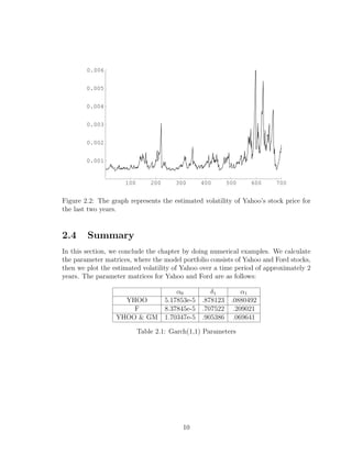
was evident in 2.2, Garch volatility estimates suffer from significant variability. As
such, there are ways to mitigate this problem in order to arrive at a much closer
approximation to the true covariance matrix. The problem itself, is known as Bayesian
state estimation, and the problem of Bayesian estimation is to estimate the underlying
value of an unobservable quantity using indirect observations. The dynamics of the
underlying variable, in this case the covariance matrix, is known before hand, while
the observation model is also known before hand. Using Bayesian Estimation, one
can filter the ”noise” from the Garch volatilities.
The problem is very simple to state in mathematical terms, however, it is not a
trivial matter finding a solution. First, following from Gordon et al. [9], let Zt ∈ Rq
be the observation vector at time t, Θt ∈ Rn
be the unobservable quantity at time t,
Wt ∈ Rm
and Vt ∈ Rp
be random vectors, f : Rn
× Rm
−→Rn
, g : Rn
× Rp
−→Rq
. Then
the transition equation is
Θt = f(Θt, Wt) (3.1.1)
and the observation equation is
Zt = g(Θt, Vt) (3.1.2)
The random variables Wt, Vt are zero mean, white noises, and the distributions of Wt
and Vt are assumed to be known. Let Dt = {Z1, . . . , Zt}.
The goal of Bayesian estimation is to find the posterior density, p(Θt|Dt). This
probability density can be calculated recursively, assuming at time t − 1 the density
p(Θt−1|Dt−1) is known, by first the prediction stage
p(Θt|Dt−1) = p(Θt|Θt−1)p(Θt−1|Dt−1)dΘt−1
11

16. followed by the update stage via Bayes rule
p(Θt|Dt) =
p(Zt|Θt)p(Θt|Dt−1)
p(Zt|Θt)p(Θt|Dt−1)dΘt
The densities p(Θt|Θt−1) and p(Zt|Θt) are derived directly from 3.1.1 and 3.1.2, re-
spectively. After the updating stage, the filtered value of Θt is calculated from the
posterior distribution by taking the expectation
˜Θt = E[Θt|Dt] = Θtp(Θt|Dt)dΘt
The difficulty in computing these filtering equations lie in the evaluation of the
integrals in the prediction and updating stages. For most cases, no analytical so-
lution exists. Only when f(Θt, Wt) and g(Θt, Vt) are linear functions, and Wt and
Vt are gaussian white noises. If the model falls under those set of restrictions then
the solution is the famous Kalman Filter, which is very simple, yet elegant set of
difference equations [10]. For our situation, as we will be shown later in the chapter,
our f(Θt, Wt) and g(Θt, Vt) are nonlinear, which precludes it from a Kalman Filter
solution. One way of dealing with nonlinearity is to approximate 3.1.1 and 3.1.2 and
then use the Kalman filter, see [10]. On the other hand, Fearnhead [8] suggests that
approximating non-Gaussian densities with Gaussian ones has the potential to cause
the filter to diverge. Hence, a new method is needed to deal with this problem.
3.2 Particle Filter
The filter we use in this paper is a simple particle filter called the Sample Importance
Resampling filter, also known as the Bayesian bootstrap filter. The algorithm uses
random samples and a likelihood function to approximate the posterior distribution
p(Θt|Dt). The algorithm, from [8], is as follows
1. Initialization Initialize the filter by sampling N particles, {Θ
(i)
0 }N
i=1, from
p(Θ0).
2. Prediction(step t) Assuming that Θ
(i)
t−1 is distributed according to p(Θt−1|Dt−1),
generate the set of points {Θ
(i)
t|t−1}N
i=1 via the equation
Θ
(i)
t|t−1 = f(Θ
(i)
t−1, W
(i)
t )
where W
(i)
t are inpendently, identically distributed random variables with prob-
ability density p(Wt).
12

17. 3. Filtration Assign probability weights qi
t to each Θ
(i)
t according to the equation
qi
t =
p(Zt|Θ
(i)
t|t−1)
N
j=1 p(Zt|Θ
(j)
t|t−1)
Then sample {Θ
(j)
t }N
j=1 from the distribution
p(Θ
(j)
t = Θ
(i)
t|t−1) = qi
t
The theoretical justification for this algorithm can be found in [8]. The benefit in
using this specification is that there are no restrictions on 3.1.1 or 3.1.2, or on the
distributions of Wt and Vt. But, the disadvantage of using this algorithm is the high
computational cost necessary to generate a sufficiently close approximation to the
posterior distribution.
In this paper we use the particle filter to estimate Σt from 2.3.6, where the ob-
servation vector is the vector of returns of a portfolio of stocks. So, notation wise,
Θt = Σt and Zt = Yt. The transition equation is derived from 2.3.6. By hypothe-
sis E[YtYt ] = Σt, so if Wt ∼ N(0, I) and define σt such that σtσt = Σt, then the
transition equation for Σt is
Σt = C + B ⊗ Σt−1 + A ⊗ σt−1Wt−1Wt−1σt−1 (3.2.1)
The observation likelihood function, p(Σt|Yt), where Np is the number of stocks, is
p(Σt|Yt) = [(2π)Np
|Σt|]− 1
2 exp −
1
2
Yt Σ−1
t Yt (3.2.2)
We used the sample covariance matrix as the initial starting point for the filter.
3.3 Summary
Finally, given the historical returns of a portfolio of stocks, one can estimate the
covariance matrix using a combination of a multivariate GARCH specification and
bayesian filtering theory. The following is a brief synopsis of the procedure
1. Estimate the parameter matrices A, B, C using the methods in chapter 2
2. Then initialize the SIR filter at the sample covariance matrix
Using this procedure one can filter out the measurement noise from the observations,
a technique frequently used in the engineering disciplines. As long as the parameter
matrices are properly conditioned, the estimated covariance matrices will be positive
definite.
13

18. Appendix A
Quasi-Newton Method
In this section, we present an iterative procedure to find a local extremum, θ∗
∈ Rm
,
of a function f : Rm
−→R. The method we use in this paper to find the minimum of
f(θ) is the variable metric method, otherwise known as the quasi-newton method.
More specifically, since we will not use the hessian, we will use the BFGS algorithm
detailed in [12]. Let Hi be the ith approximation of the inverse of the hessian of f(θ).
Let fi = f(θi), H0 be the identity matrix and θ0 be in the neighborhood of θ∗
,
where f(θ) is approximately quadratic. Then the algorithm is as follows:
θi+1 = θi − Hi fi (A.0.1)
Hi+1 = Hi +
(θi+1 − θi) ⊗ (θi+1 − θi)
(θi+1 − θi) ( fi+1 − fi)
− (A.0.2)
[Hi( fi+1 − fi)] ⊗ [Hi( fi+1 − fi)]
( fi+1 − fi) Hi( fi+1 − fi)
+ [( fi+1 − fi) Hi( fi+1 − fi)]u ⊗ u
where u is defined as the vector
u =
θi+1 − θi
(θi+1 − θi) ( fi+1 − fi)
−
Hi( fi+1 − fi)
( fi+1 − fi) Hi( fi+1 − fi)
As θi−→θ∗
, BFGS enjoys the quadratic convergence rate of newton’s method with the
known hessian. However, this algorithm requires a relatively accurate initial guess.
To find a decent approximation we use the steepest descent algorithm, which is just
newton’s method with the assumption that the hessian is equal to a constant times the
identity matrix. In this section, we present the pose the question of finding positive
semidefinite matrices given a suitable estimate that is not positive semidefinite.
14

19. Appendix B
Finding Nearest Correlation
Matrix
In this section, we summarize the algorithm used in Ledoit et al. [11] to find the
closest fitting positive, semdefinite matrix to the current estimated matrix. Given a
symmetric matrix A with the property diag(A) > 0, the algorithm finds a symmetric,
positive, semidefinite matrix M with diag(M) = diag(A), such that quantity A −
M F , where F is the Frobenius norm, is minimized. First, start with the 1st row and
column.
A =
a11 a
a ¯A
M =
a11 m
m ˜M
where diag(M) = diag(A) and M = M . Define P as the following
P =
ρ x
0 In−1
We iterate be setting
˘M = PMP =
ρ2
a11 + 2ρx m + x ˜Mx ρm + x ¯M
ρm + ˜Mx ˜M
(B-1)
For each iteration the quantity a − (ρm + ˜Mx) must be minimized subject to the
constraint that ρ2
a11+2ρx m+x ˜Mx = a11 Ledoit et al. [11] derive a simple algorithm
to this. Let λ, F, Fλ be scalars, then the algorithm is as follows
1. Initialize λ = 0 (starting point is arbitrary).
2. x = ( ˜M2
+ λ ˜M)−1
( ˜Mb − λρm)
3. Set F = ρ2
a11 +2ρx m+x ˜Mx−a11 and Fλ = −2(ρm+ ˜Mx) ( ˜M2
+λ ˜M)−1
(ρm+
˜Mx)
15

20. 4. λ = λ − F
Fλ
5. Repeat steps 2.-4. until satisfactory convergence.
Rho is usual set as a constant between zero and one, say .5. This way det( ˘M) =
ρ2
det(M), which means M converges to a singular matrix at the rate ρ2
.
16

21. Bibliography
[1] F. Black and M. Scholes, The pricing of options and corporate liabilities, The
Journal of Political Economy 81 (1973), 637–654.
[2] T. Bollerslev, R. F. Engle, and D. Nelson, Handbook of econometrics volume 4,
Elsevier Science Pub Co, New York, NY, USA, 1999.
[3] T. Bollerslev, R. F. Engle, and J. M. Wooldridge, Capital asset pricing model
with time-varying covariances, Journal of Political Economy 96 (1988), 116–131.
[4] Tim Bollerslev, Generalized autoregressive conditional heteroskedasticity, Journal
of Econometrics 31 (1986), 307–327.
[5] Robert F. Engle, Autoregressive conditional heteroscedasticity with estimates of
the variance of united kingdom inflation, Econometrica 50 (1984), 987–1008.
[6] , Dynamic conditional correlation - a simple class of multivariate garch
models, Jul 1999.
[7] , Garch101: The use of arch/garch models in applied econometrics, The
Journal of Economic Perspectives 15 (2001), 157–168.
[8] P. Fearnhead, Sequential monte carlo methods in filter theory, Ph.D. thesis, Ox-
ford, 1998.
[9] N. J. Gordon, D. J. Salmond, and A. F. M. Smith, Novel approach to
nonlinear/non-gaussian bayesian state estimation, IEE Proceedings-F 140
(1993), 107–113.
[10] R. E. Kalman, A new approach to linear filtering and prediction problems, Trans-
action of the ASME, 1960, pp. 35–45.
[11] O. Ledoit, P. Santa-Clara, and M. Wolf, Flexible multivariate garch modeling
with an application to international stock markets, The Review of Economics
and Statistics 85 (2003), 735–747.
17

22. [12] W. H. Press, S. A. Teukolsky, W. T. Vetterling, and B. P. Flannery, Numerical
recipes in c: The art of scientific computing, Cambridge University Press, New
York, NY, USA, 1992.
18

23. Name of Candidate: Joel DeJesus
Birth Date: 10 October 1984
Birth Place: N¨urnburg, Germany
Address: 1000 SW 62blvd Gainesville, FL