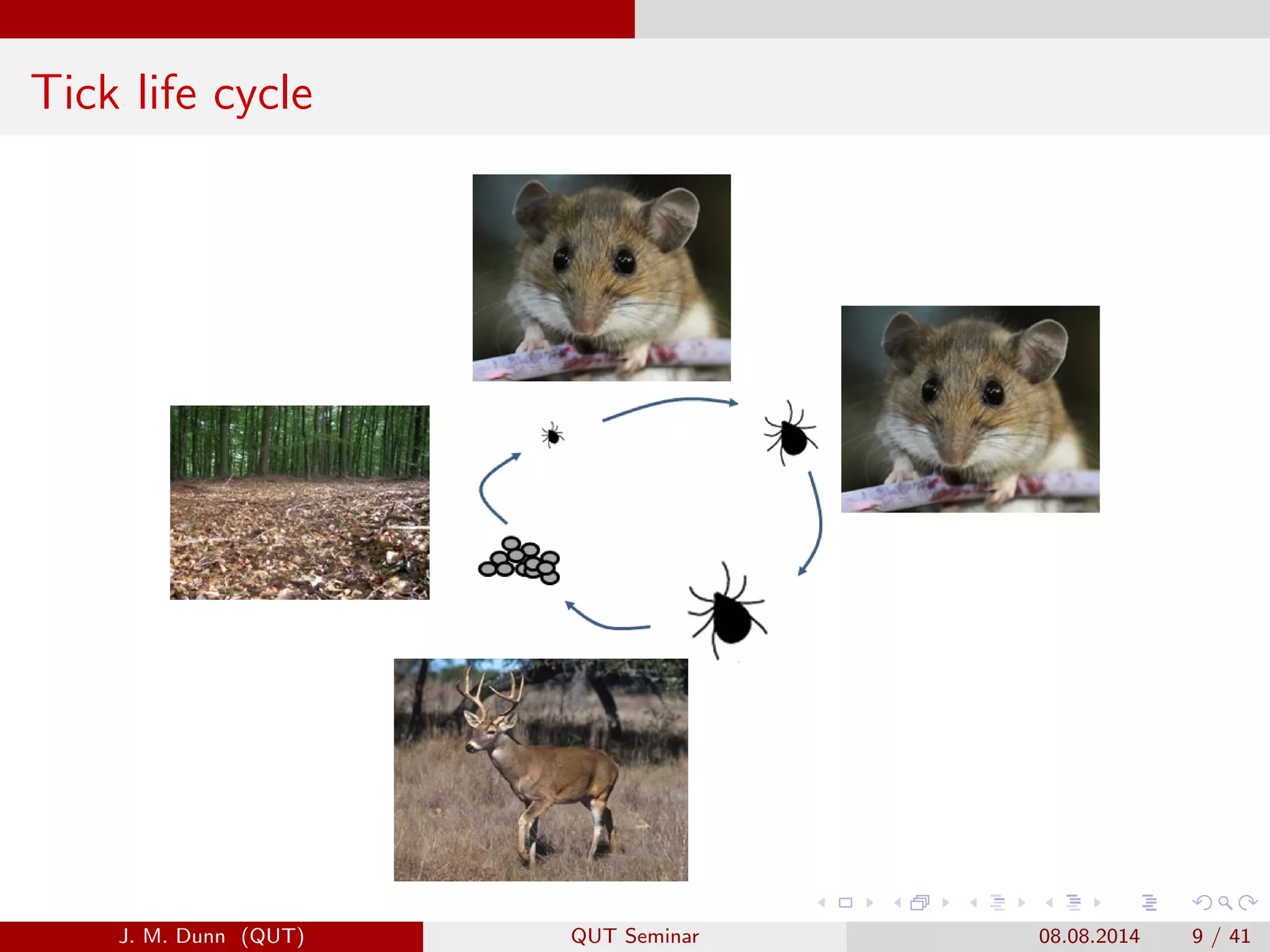
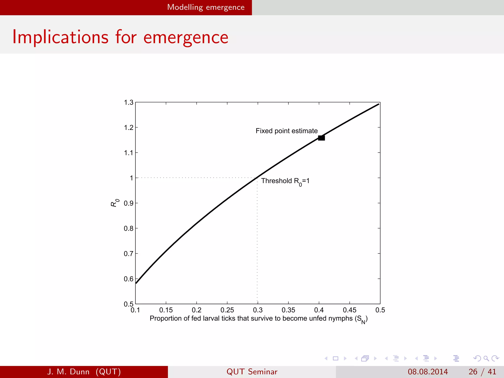
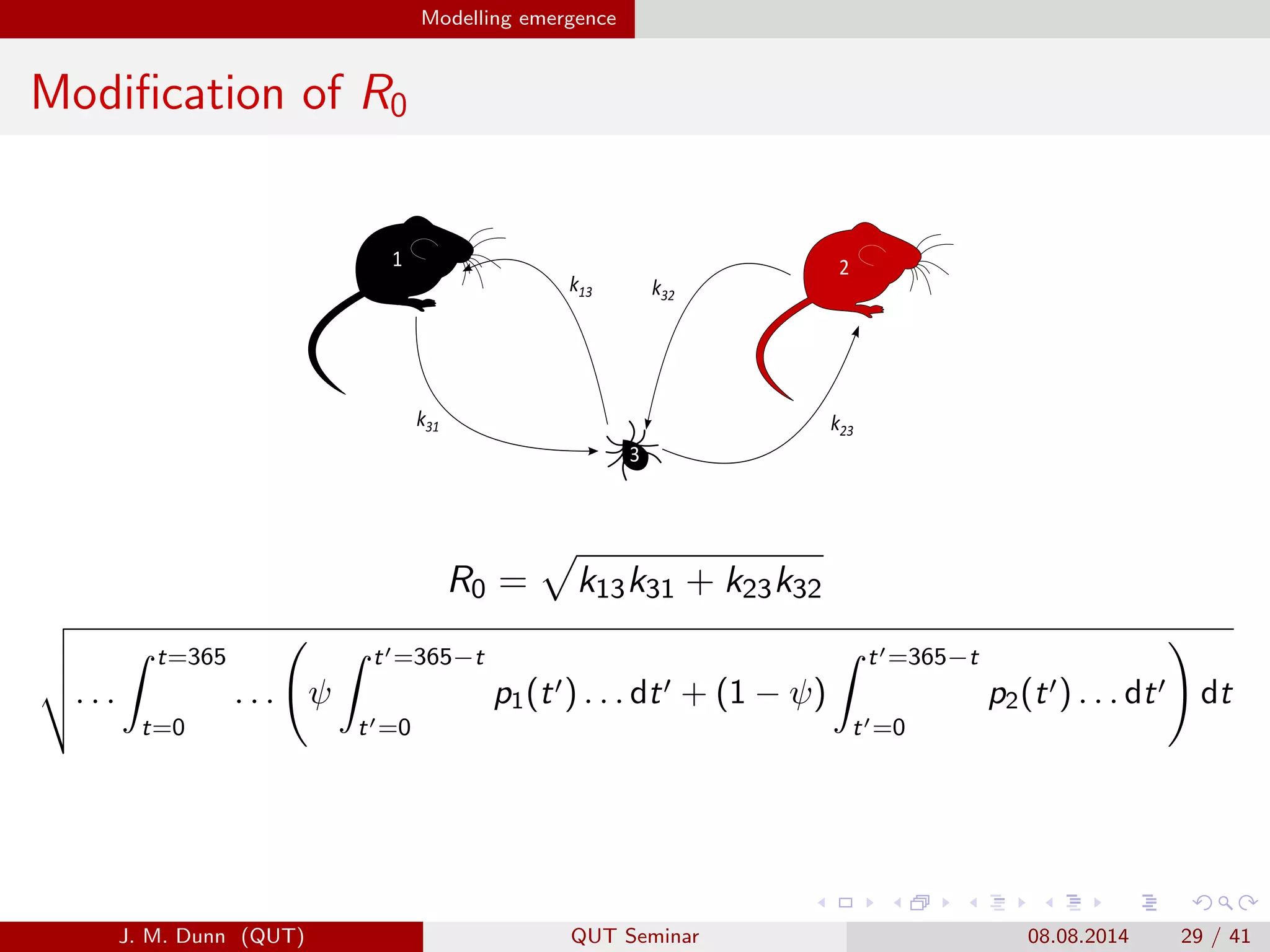
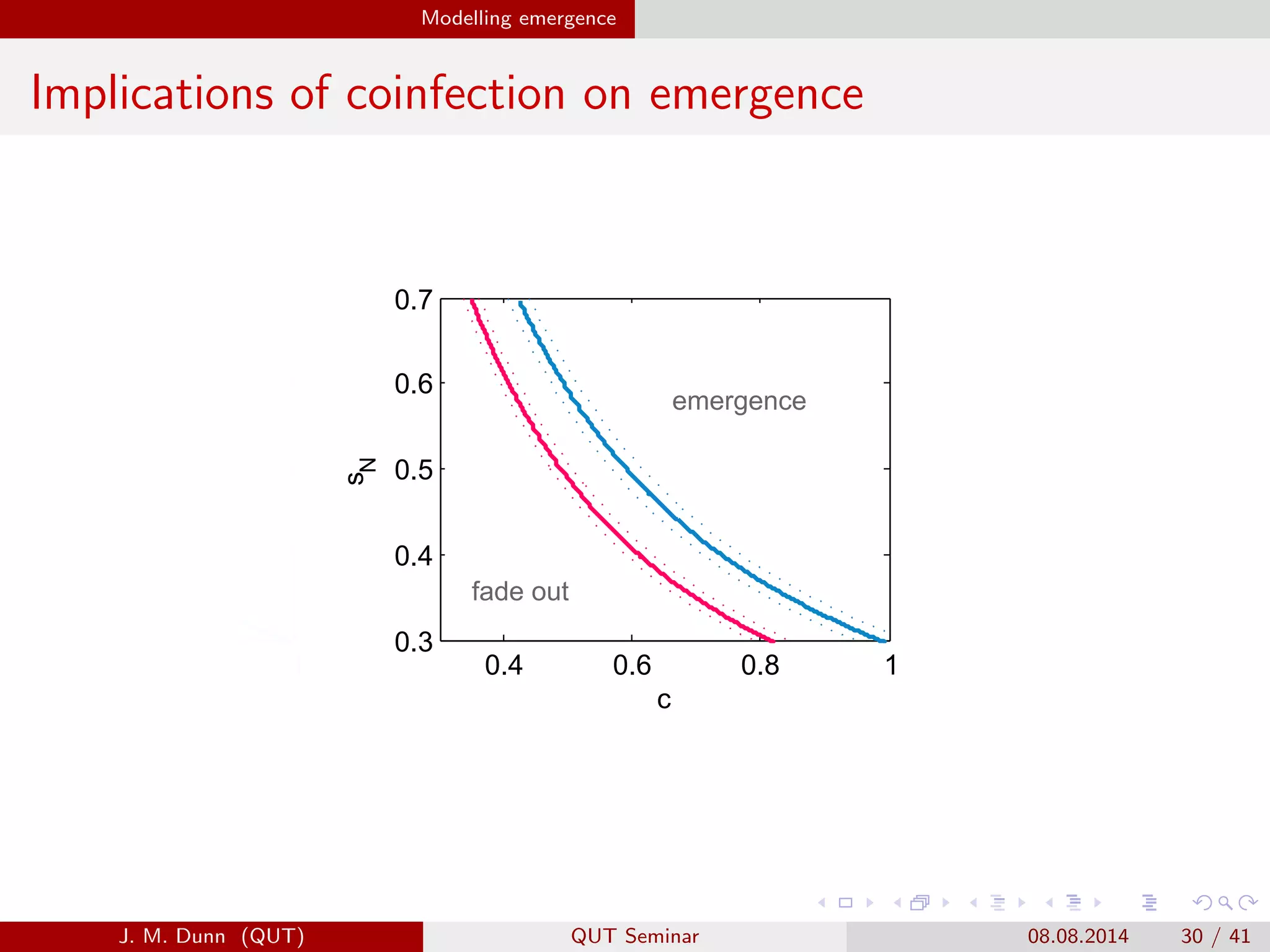
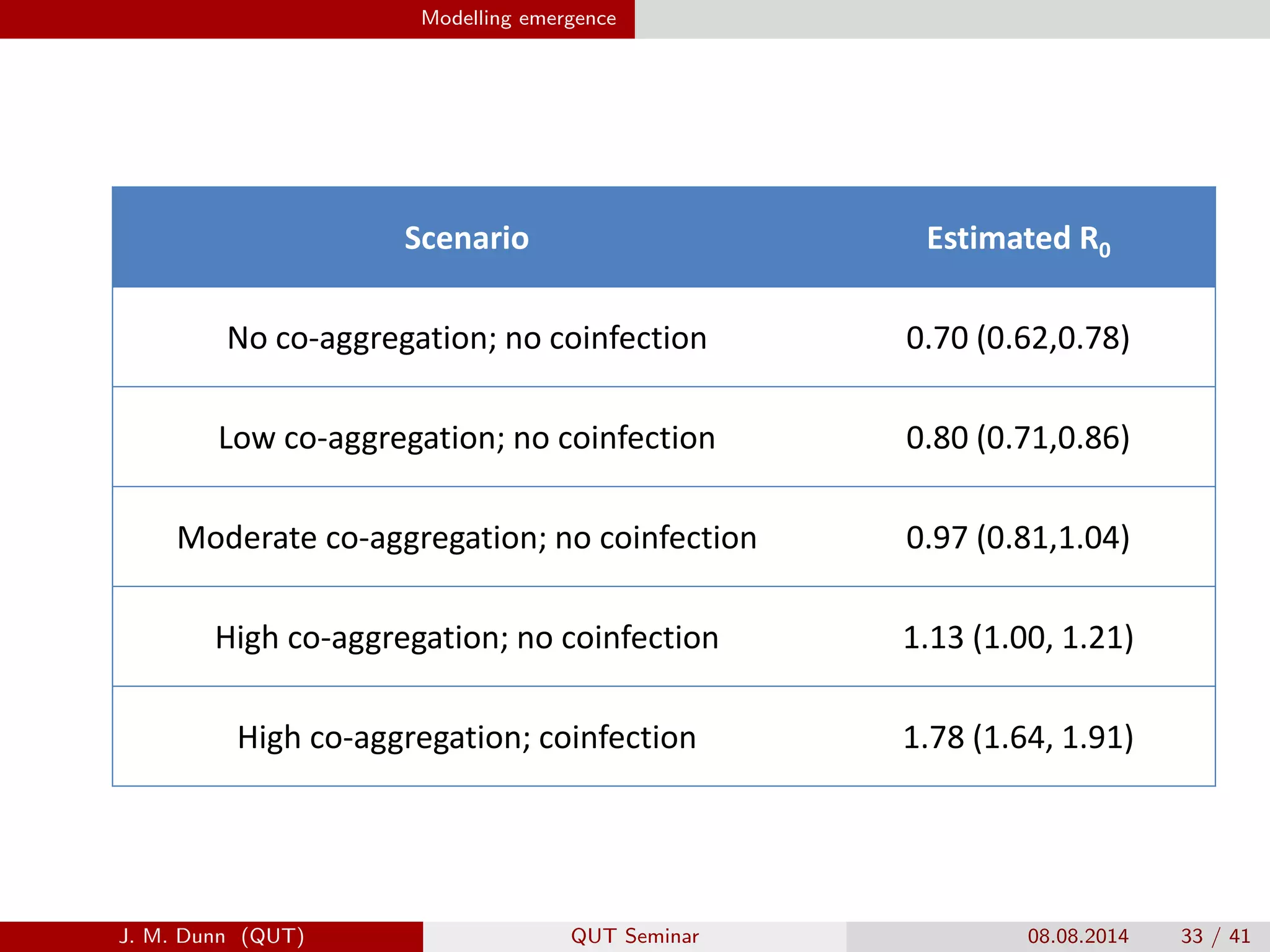
The Mathematical Epidemiology of Human Babesiosis in
the North-Eastern United States
Jessica Margaret Dunn, Dr. Stephen Davis (RMIT), Dr. Andrew
Stacey (RMIT), Assoc. Prof. Maria Diuk-Wasser (Yale/Columbia)
J. M. Dunn (QUT) QUT Seminar 08.08.2014 1 / 41
J. M. Dunn (QUT) QUT Seminar 08.08.2014 2 / 41
Tick-borne disease in the USA
The geographical range of tick-borne diseases are expanding. There are
seven emerging tick diseases:
Lyme disease
Human babesiosis
Human anaplasmosis
Powassan
Deer tick encephalitis
B. miyamotoi borreliosis
Deer tick ehrlichiosis
J. M. Dunn (QUT) QUT Seminar 08.08.2014 3 / 41
Lyme Disease (Borrelia burgdorferi)
J. M. Dunn (QUT) QUT Seminar 08.08.2014 4 / 41
Human Babesiosis (Babesia microti)
Reported cases of Human Babesiosis – United States, 2011
J. M. Dunn (QUT) QUT Seminar 08.08.2014 5 / 41
Hosts
White-footed mice (Peromyscus leucopus) Tick (Ixodes scapularis)
J. M. Dunn (QUT) QUT Seminar 08.08.2014 6 / 41
Research Objective
To identify the key factors driving human babesiosis (B. microti) and
Lyme disease (B. burgdorferi) in endemic sites, and their expansion
into new areas in the north-eastern United States.
J. M. Dunn (QUT) QUT Seminar 08.08.2014 7 / 41
Mathematical Modelling Challenges
Deriving mathematical models of tick-borne disease transmission is
notoriously difficult!
Multiple hosts (competent and non-competent)
Tick life-cycle (biting rate)
Multiple tranmission routes
Multiple pathogens
J. M. Dunn (QUT) QUT Seminar 08.08.2014 8 / 41
Tick life cycle
J. M. Dunn (QUT) QUT Seminar 08.08.2014 9 / 41
Tick-phenology
Densities-Northeast
Weeks
Density
0 5 10 15 20 25 30 35 40 45 50
0
50
100
150
200
250
300
350
400
450
500 Larvae
Nymphs
Adults
J. M. Dunn (QUT) QUT Seminar 08.08.2014 10 / 41
Tick-borne pathogen transmission routes
J. M. Dunn (QUT) QUT Seminar 08.08.2014 11 / 41
Modelling challenges
The modelling challenge then becomes to one of incorporating these
complexities whilst maintaining a model that:
1 is representative of the transmission cycle
2 can be used with field data which will provide meaningful estimates of
the parameters
3 has a minimal number of parameters to ensure the model can be
adequately analysed
J. M. Dunn (QUT) QUT Seminar 08.08.2014 12 / 41
Overview
Model emergence
- Identify the factors driving emergence
- Identify control measures
Model the risk to humans
- Incorporate the identified factors
- Analyse changes in risk
J. M. Dunn (QUT) QUT Seminar 08.08.2014 13 / 41
Modelling emergence
Modelling emergence
The basic Reproduction number, R0
In single host systems, R0 is the expected number of secondary cases
produced by one infectious individual in a fully susceptible population.
R0 = 1 provides a threshold condition:
pathogen will spread R0 > 1
pathogen will fade out R0 < 1
J. M. Dunn (QUT) QUT Seminar 08.08.2014 14 / 41
Modelling emergence
R0 for multiple hosts
Next generation Matrix (NGM) (Diekmann and Heasterbeek)
Define kij as the expected number of new cases that have state at
infection i caused by one individual at state at infection j, during its whole
infectious period.
For example given 2 host types i and j there are four possibilities:
K = (kij ) =
k11 k12
k21 k22
R0 is the dominant eigenvalue of the NGM such that
vk+1 = Kvk
J. M. Dunn (QUT) QUT Seminar 08.08.2014 15 / 41
Modelling emergence
NGM for tick-borne pathogens
J. M. Dunn (QUT) QUT Seminar 08.08.2014 16 / 41
Modelling emergence
Reduction for US Lyme and Human Babesiosis
J. M. Dunn (QUT) QUT Seminar 08.08.2014 17 / 41
Modelling emergence
NGM for US Lyme and Human Babesiosis
J. M. Dunn (QUT) QUT Seminar 08.08.2014 18 / 41
Modelling emergence
Quantifying R0
J. M. Dunn (QUT) QUT Seminar 08.08.2014 19 / 41
Modelling emergence
Internal functions of R0
Tick Phenology
0 50 100 150 200 250 300 350
Day
Mean nymph burden
Mean larvae burden
Representativemeantick
countpermouse
52050
μ
H
τ
J. M. Dunn (QUT) QUT Seminar 08.08.2014 20 / 41
Modelling emergence
Block Island
Connecticut
100 250150 200 100 150 200 250
100 150 200 250100 150 200 250
0
1
5
20
50
150
0
1
5
20
50
150150
50
20
5
1
0
150
50
20
5
1
0
Day of year Day of year
LarvaltickburdenLarvaltickburden
NymphaltickburdenNymphaltickburden
J. M. Dunn (QUT) QUT Seminar 08.08.2014 21 / 41
Modelling emergence
Brunner and Ostfeld (2008)
¯ZN(t) = HNe
−1
2
ln
(t−τN )
µN
/σN
2
if t ≥ τN;
0 otherwise
¯ZL(t) =



HE e
−1
2
t−τE
µE
2
if t ≤ τL;
HLe
−1
2
ln
(t−τL)
µL
2
+ HE e
−1
2
t−τE
µE
2
otherwise
J. M. Dunn (QUT) QUT Seminar 08.08.2014 22 / 41
Modelling emergence
Internal functions of R0
Efficiency of transmissionInfectivity
Days
H
μ
p(t) = HPe
−1
2
ln t
µP
/σP
2
J. M. Dunn (QUT) QUT Seminar 08.08.2014 23 / 41
Modelling emergence
Global Sensitivity Analysis of R0
Ranks the parameters by their contribution to the variation of R0 using
Sobol’s indices:
Main effect: calculates the effect of parameter xi on R0 fixing all
other variables
Total effect: includes the main effect for xi plus all other interaction
involving xi .
J. M. Dunn (QUT) QUT Seminar 08.08.2014 24 / 41
Modelling emergence
Global Sensitivity Results
0
0.1
0.2
0.3
0.4
0.5
0.6
0.7
0.8
0.9
1
Parameter
Sobol’sfIndices
MainfEffect
TotalfEffect
H τ μ σ τ H τ μ H μ σ H Dq ρ σμ s cN N N N L L L L P P PLE E E NN
J. M. Dunn (QUT) QUT Seminar 08.08.2014 25 / 41
Modelling emergence
Implications for emergence
0.1 0.15 0.2 0.25 0.3 0.35 0.4 0.45 0.5
0.5
0.6
0.7
0.8
0.9
1
1.1
1.2
1.3
Proportion of fed larval ticks that survive to become unfed nymphs (S
N
)
R
0
Threshold R
0
=1
Fixed point estimate
J. M. Dunn (QUT) QUT Seminar 08.08.2014 26 / 41
Modelling emergence
Implications for control
Given, ¯R0 = 1.57
Vaccination requirements (Roberts, 2003)
V = 1 −
1
R2
0
≈ 60%
J. M. Dunn (QUT) QUT Seminar 08.08.2014 27 / 41
Modelling emergence
The Coinfection Story
J.M. Dunn et al. Borrelia burgdorferi enhances the enzootic establishment of
Babesia microti in the northeastern United States, PLOS ONE(2014).
J. M. Dunn (QUT) QUT Seminar 08.08.2014 28 / 41
Modelling emergence
Modification of R0
k13
k31
k13
k31 k32
k23
k32
k23
White-footedm1:
White-footedm2:
Tickainfectedaw3:
Ka= 0 0
0 0
0
1 2
3
R0 = k13k31 + k23k32
. . .
t=365
t=0
. . . ψ
t =365−t
t =0
p1(t ) . . . dt + (1 − ψ)
t =365−t
t =0
p2(t ) . . . dt dt
J. M. Dunn (QUT) QUT Seminar 08.08.2014 29 / 41
Modelling emergence
Implications of coinfection on emergence
0.6 0.8 1
c
0.4 0.6 0.8 1
0.3
0.4
0.5
c
0.6 0.8 1
c
0.4 0.6 0.8 1
0.3
0.4
0.5
0.6
0.7
c
sN
B. microti
B. microti C8B. Burgdorferi BL2068
fade8out
fade8out
emergence emergence
80w8B. burgdorferi8BL2068prevalence
in8mice
J. M. Dunn (QUT) QUT Seminar 08.08.2014 30 / 41
Modelling emergence
Timing is everything!120 140 160 180 200 220 240 260 280 300
0
5
120 140 160 180 200 220 240 260 280 300
0
5
10
15
Re
ouseProportion3of3infected3larval3ticks3per3mouse
Representative3mean3tick3count3per3mouse
Connecticut
3330.233333330.1
Mean nymph burden
Mean larvae burden
Babesia3+3Borrelia
Babesia
3333333333333333333333333333330.93333330.83333330.73333330.63333330.53333330.43333330.333333330.233333330.1
J. M. Dunn (QUT) QUT Seminar 08.08.2014 31 / 41
Modelling emergence
Coinfection is not the whole story!
Accounting for aggregation on hosts
k13
k13
32
1
5
4
2
k51
k15
k12
k21
k14
k41
2: High aggregation white footed mouse
- infected with Bb
4: Low aggregation white footed mouse
- infected with Bb
3: High aggregation white footed mouse
- infected with Bm
5: Low aggregation white footed mouse
- infected with Bm
R0 = k12k21 + k12k21 + k13k31 + k14k41 + k15k51
J. M. Dunn (QUT) QUT Seminar 08.08.2014 32 / 41
Modelling emergence
Scenario Estimated R0
No co-aggregation; no coinfection 0.70 (0.62,0.78)
Low co-aggregation; no coinfection 0.80 (0.71,0.86)
Moderate co-aggregation; no coinfection 0.97 (0.81,1.04)
High co-aggregation; no coinfection 1.13 (1.00, 1.21)
High co-aggregation; coinfection 1.78 (1.64, 1.91)
J. M. Dunn (QUT) QUT Seminar 08.08.2014 33 / 41
Modelling emergence
Conclusions
Epidemiological:
Values of R0 are consistently low 1 < R0 < 3
Transmission efficiency drives emergence
Timing is everything!
Mathematical:
Models are mechanistic, transparent, linked directly with field data
Step towards a model for more complicated tick-borne pathogens
First such model that that assesses the importance of (i) coinfection
and (ii) aggregation
J. M. Dunn (QUT) QUT Seminar 08.08.2014 34 / 41
Modelling emergence
Questions?
J. M. Dunn (QUT) QUT Seminar 08.08.2014 35 / 41
Modelling risk
Modelling risk to humans
Risk is directly proportional to the infection prevalence in nymphal ticks.
Compartment type SIR Model: (S)usceptibles to (I)nfectives to
(R)ecovered
J. M. Dunn (QUT) QUT Seminar 08.08.2014 36 / 41
Modelling risk
Three generation based compartments:
Sk(t), Ik(t) and Ck(t)
dSk
dt
= −βk(t)Sk
dIk
dt
= βk(t)Sk − γI
dCk
dt
= γI
J. M. Dunn (QUT) QUT Seminar 08.08.2014 37 / 41
Modelling risk
Force of Infection
The force of infection is related to the unfed nymphs from the previous
year k − 1
βk(t) =
1
DN
νk
¯ZN(t)qN.
with the proportion of infected unfed nymphs, νk, in year k is given by
νk =
365
0
aL(t)¯p
Ik−1
Nk−1
dt
J. M. Dunn (QUT) QUT Seminar 08.08.2014 38 / 41
Modelling risk
Accounting for infectivity of hosts p(t)
J. M. Dunn (QUT) QUT Seminar 08.08.2014 39 / 41
Modelling risk
dSk
dt
= −βk(t)Sk + b(t)Nk − (µ +
Nk
K
)Sk
dIk,1
dt
= βk(t)Sk − (µ +
Nk
K
)Ik,1 − γI1
dIk,2
dt
= γI1 − (µ +
Nk
K
)Ik,2 − γI2
dIk,3
dt
= γI2 − (µ +
Nk
K
)Ik,3 − γI3
dIk,4
dt
= γI3 − (µ +
Nk
K
)Ik,4 − γI4
dIk,5
dt
= γI4 − (µ +
Nk
K
)Ik,5 − γI5
dIk,6
dt
= γI5 − (µ +
Nk
K
)Ik,6 − γI6
dCk
dt
= γI6 − (µ +
Nk
K
)C
J. M. Dunn (QUT) QUT Seminar 08.08.2014 40 / 41
Modelling risk
νk =
365
0
aL(t) ¯p1
Ik−1,1
Nk−1
+ ¯p2
Ik−1,2
Nk−1
+ ¯p3
Ik−1,3
Nk−1
+ ¯p4
Ik−1,4
Nk−1
+ ¯p5
Ik−1,5
Nk−1
+ ¯p6
Ik−1,6
Nk−1
dt
0 5 10 15 20 25 30
0
0.01
0.02
0.03
0.04
0.05
0.06
0.07
0.08
0.09
time (years)
Proportionofinfectedfedlarvae
J. M. Dunn (QUT) QUT Seminar 08.08.2014 41 / 41

The Mathematical Epidemiology of Human Babesiosis in the North-Eastern United States - Jessica Dunn, QUT

  • 1.
    The Mathematical Epidemiologyof Human Babesiosis in the North-Eastern United States Jessica Margaret Dunn, Dr. Stephen Davis (RMIT), Dr. Andrew Stacey (RMIT), Assoc. Prof. Maria Diuk-Wasser (Yale/Columbia) J. M. Dunn (QUT) QUT Seminar 08.08.2014 1 / 41
  • 2.
    J. M. Dunn(QUT) QUT Seminar 08.08.2014 2 / 41
  • 3.
    Tick-borne disease inthe USA The geographical range of tick-borne diseases are expanding. There are seven emerging tick diseases: Lyme disease Human babesiosis Human anaplasmosis Powassan Deer tick encephalitis B. miyamotoi borreliosis Deer tick ehrlichiosis J. M. Dunn (QUT) QUT Seminar 08.08.2014 3 / 41
  • 4.
    Lyme Disease (Borreliaburgdorferi) J. M. Dunn (QUT) QUT Seminar 08.08.2014 4 / 41
  • 5.
    Human Babesiosis (Babesiamicroti) Reported cases of Human Babesiosis – United States, 2011 J. M. Dunn (QUT) QUT Seminar 08.08.2014 5 / 41
  • 6.
    Hosts White-footed mice (Peromyscusleucopus) Tick (Ixodes scapularis) J. M. Dunn (QUT) QUT Seminar 08.08.2014 6 / 41
  • 7.
    Research Objective To identifythe key factors driving human babesiosis (B. microti) and Lyme disease (B. burgdorferi) in endemic sites, and their expansion into new areas in the north-eastern United States. J. M. Dunn (QUT) QUT Seminar 08.08.2014 7 / 41
  • 8.
    Mathematical Modelling Challenges Derivingmathematical models of tick-borne disease transmission is notoriously difficult! Multiple hosts (competent and non-competent) Tick life-cycle (biting rate) Multiple tranmission routes Multiple pathogens J. M. Dunn (QUT) QUT Seminar 08.08.2014 8 / 41
  • 9.
    Tick life cycle J.M. Dunn (QUT) QUT Seminar 08.08.2014 9 / 41
  • 10.
    Tick-phenology Densities-Northeast Weeks Density 0 5 1015 20 25 30 35 40 45 50 0 50 100 150 200 250 300 350 400 450 500 Larvae Nymphs Adults J. M. Dunn (QUT) QUT Seminar 08.08.2014 10 / 41
  • 11.
    Tick-borne pathogen transmissionroutes J. M. Dunn (QUT) QUT Seminar 08.08.2014 11 / 41
  • 12.
    Modelling challenges The modellingchallenge then becomes to one of incorporating these complexities whilst maintaining a model that: 1 is representative of the transmission cycle 2 can be used with field data which will provide meaningful estimates of the parameters 3 has a minimal number of parameters to ensure the model can be adequately analysed J. M. Dunn (QUT) QUT Seminar 08.08.2014 12 / 41
  • 13.
    Overview Model emergence - Identifythe factors driving emergence - Identify control measures Model the risk to humans - Incorporate the identified factors - Analyse changes in risk J. M. Dunn (QUT) QUT Seminar 08.08.2014 13 / 41
  • 14.
    Modelling emergence Modelling emergence Thebasic Reproduction number, R0 In single host systems, R0 is the expected number of secondary cases produced by one infectious individual in a fully susceptible population. R0 = 1 provides a threshold condition: pathogen will spread R0 > 1 pathogen will fade out R0 < 1 J. M. Dunn (QUT) QUT Seminar 08.08.2014 14 / 41
  • 15.
    Modelling emergence R0 formultiple hosts Next generation Matrix (NGM) (Diekmann and Heasterbeek) Define kij as the expected number of new cases that have state at infection i caused by one individual at state at infection j, during its whole infectious period. For example given 2 host types i and j there are four possibilities: K = (kij ) = k11 k12 k21 k22 R0 is the dominant eigenvalue of the NGM such that vk+1 = Kvk J. M. Dunn (QUT) QUT Seminar 08.08.2014 15 / 41
  • 16.
    Modelling emergence NGM fortick-borne pathogens J. M. Dunn (QUT) QUT Seminar 08.08.2014 16 / 41
  • 17.
    Modelling emergence Reduction forUS Lyme and Human Babesiosis J. M. Dunn (QUT) QUT Seminar 08.08.2014 17 / 41
  • 18.
    Modelling emergence NGM forUS Lyme and Human Babesiosis J. M. Dunn (QUT) QUT Seminar 08.08.2014 18 / 41
  • 19.
    Modelling emergence Quantifying R0 J.M. Dunn (QUT) QUT Seminar 08.08.2014 19 / 41
  • 20.
    Modelling emergence Internal functionsof R0 Tick Phenology 0 50 100 150 200 250 300 350 Day Mean nymph burden Mean larvae burden Representativemeantick countpermouse 52050 μ H τ J. M. Dunn (QUT) QUT Seminar 08.08.2014 20 / 41
  • 21.
    Modelling emergence Block Island Connecticut 100250150 200 100 150 200 250 100 150 200 250100 150 200 250 0 1 5 20 50 150 0 1 5 20 50 150150 50 20 5 1 0 150 50 20 5 1 0 Day of year Day of year Day of year Day of year LarvaltickburdenLarvaltickburden NymphaltickburdenNymphaltickburden J. M. Dunn (QUT) QUT Seminar 08.08.2014 21 / 41
  • 22.
    Modelling emergence Brunner andOstfeld (2008) ¯ZN(t) = HNe −1 2 ln (t−τN ) µN /σN 2 if t ≥ τN; 0 otherwise ¯ZL(t) =    HE e −1 2 t−τE µE 2 if t ≤ τL; HLe −1 2 ln (t−τL) µL 2 + HE e −1 2 t−τE µE 2 otherwise J. M. Dunn (QUT) QUT Seminar 08.08.2014 22 / 41
  • 23.
    Modelling emergence Internal functionsof R0 Efficiency of transmissionInfectivity Days H μ p(t) = HPe −1 2 ln t µP /σP 2 J. M. Dunn (QUT) QUT Seminar 08.08.2014 23 / 41
  • 24.
    Modelling emergence Global SensitivityAnalysis of R0 Ranks the parameters by their contribution to the variation of R0 using Sobol’s indices: Main effect: calculates the effect of parameter xi on R0 fixing all other variables Total effect: includes the main effect for xi plus all other interaction involving xi . J. M. Dunn (QUT) QUT Seminar 08.08.2014 24 / 41
  • 25.
    Modelling emergence Global SensitivityResults 0 0.1 0.2 0.3 0.4 0.5 0.6 0.7 0.8 0.9 1 Parameter Sobol’sfIndices MainfEffect TotalfEffect H τ μ σ τ H τ μ H μ σ H Dq ρ σμ s cN N N N L L L L P P PLE E E NN J. M. Dunn (QUT) QUT Seminar 08.08.2014 25 / 41
  • 26.
    Modelling emergence Implications foremergence 0.1 0.15 0.2 0.25 0.3 0.35 0.4 0.45 0.5 0.5 0.6 0.7 0.8 0.9 1 1.1 1.2 1.3 Proportion of fed larval ticks that survive to become unfed nymphs (S N ) R 0 Threshold R 0 =1 Fixed point estimate J. M. Dunn (QUT) QUT Seminar 08.08.2014 26 / 41
  • 27.
    Modelling emergence Implications forcontrol Given, ¯R0 = 1.57 Vaccination requirements (Roberts, 2003) V = 1 − 1 R2 0 ≈ 60% J. M. Dunn (QUT) QUT Seminar 08.08.2014 27 / 41
  • 28.
    Modelling emergence The CoinfectionStory J.M. Dunn et al. Borrelia burgdorferi enhances the enzootic establishment of Babesia microti in the northeastern United States, PLOS ONE(2014). J. M. Dunn (QUT) QUT Seminar 08.08.2014 28 / 41
  • 29.
    Modelling emergence Modification ofR0 k13 k31 k13 k31 k32 k23 k32 k23 White-footedm1: White-footedm2: Tickainfectedaw3: Ka= 0 0 0 0 0 1 2 3 R0 = k13k31 + k23k32 . . . t=365 t=0 . . . ψ t =365−t t =0 p1(t ) . . . dt + (1 − ψ) t =365−t t =0 p2(t ) . . . dt dt J. M. Dunn (QUT) QUT Seminar 08.08.2014 29 / 41
  • 30.
    Modelling emergence Implications ofcoinfection on emergence 0.6 0.8 1 c 0.4 0.6 0.8 1 0.3 0.4 0.5 c 0.6 0.8 1 c 0.4 0.6 0.8 1 0.3 0.4 0.5 0.6 0.7 c sN B. microti B. microti C8B. Burgdorferi BL2068 fade8out fade8out emergence emergence 80w8B. burgdorferi8BL2068prevalence in8mice J. M. Dunn (QUT) QUT Seminar 08.08.2014 30 / 41
  • 31.
    Modelling emergence Timing iseverything!120 140 160 180 200 220 240 260 280 300 0 5 120 140 160 180 200 220 240 260 280 300 0 5 10 15 Re ouseProportion3of3infected3larval3ticks3per3mouse Representative3mean3tick3count3per3mouse Connecticut 3330.233333330.1 Mean nymph burden Mean larvae burden Babesia3+3Borrelia Babesia 3333333333333333333333333333330.93333330.83333330.73333330.63333330.53333330.43333330.333333330.233333330.1 J. M. Dunn (QUT) QUT Seminar 08.08.2014 31 / 41
  • 32.
    Modelling emergence Coinfection isnot the whole story! Accounting for aggregation on hosts k13 k13 32 1 5 4 2 k51 k15 k12 k21 k14 k41 2: High aggregation white footed mouse - infected with Bb 4: Low aggregation white footed mouse - infected with Bb 3: High aggregation white footed mouse - infected with Bm 5: Low aggregation white footed mouse - infected with Bm R0 = k12k21 + k12k21 + k13k31 + k14k41 + k15k51 J. M. Dunn (QUT) QUT Seminar 08.08.2014 32 / 41
  • 33.
    Modelling emergence Scenario EstimatedR0 No co-aggregation; no coinfection 0.70 (0.62,0.78) Low co-aggregation; no coinfection 0.80 (0.71,0.86) Moderate co-aggregation; no coinfection 0.97 (0.81,1.04) High co-aggregation; no coinfection 1.13 (1.00, 1.21) High co-aggregation; coinfection 1.78 (1.64, 1.91) J. M. Dunn (QUT) QUT Seminar 08.08.2014 33 / 41
  • 34.
    Modelling emergence Conclusions Epidemiological: Values ofR0 are consistently low 1 < R0 < 3 Transmission efficiency drives emergence Timing is everything! Mathematical: Models are mechanistic, transparent, linked directly with field data Step towards a model for more complicated tick-borne pathogens First such model that that assesses the importance of (i) coinfection and (ii) aggregation J. M. Dunn (QUT) QUT Seminar 08.08.2014 34 / 41
  • 35.
    Modelling emergence Questions? J. M.Dunn (QUT) QUT Seminar 08.08.2014 35 / 41
  • 36.
    Modelling risk Modelling riskto humans Risk is directly proportional to the infection prevalence in nymphal ticks. Compartment type SIR Model: (S)usceptibles to (I)nfectives to (R)ecovered J. M. Dunn (QUT) QUT Seminar 08.08.2014 36 / 41
  • 37.
    Modelling risk Three generationbased compartments: Sk(t), Ik(t) and Ck(t) dSk dt = −βk(t)Sk dIk dt = βk(t)Sk − γI dCk dt = γI J. M. Dunn (QUT) QUT Seminar 08.08.2014 37 / 41
  • 38.
    Modelling risk Force ofInfection The force of infection is related to the unfed nymphs from the previous year k − 1 βk(t) = 1 DN νk ¯ZN(t)qN. with the proportion of infected unfed nymphs, νk, in year k is given by νk = 365 0 aL(t)¯p Ik−1 Nk−1 dt J. M. Dunn (QUT) QUT Seminar 08.08.2014 38 / 41
  • 39.
    Modelling risk Accounting forinfectivity of hosts p(t) J. M. Dunn (QUT) QUT Seminar 08.08.2014 39 / 41
  • 40.
    Modelling risk dSk dt = −βk(t)Sk+ b(t)Nk − (µ + Nk K )Sk dIk,1 dt = βk(t)Sk − (µ + Nk K )Ik,1 − γI1 dIk,2 dt = γI1 − (µ + Nk K )Ik,2 − γI2 dIk,3 dt = γI2 − (µ + Nk K )Ik,3 − γI3 dIk,4 dt = γI3 − (µ + Nk K )Ik,4 − γI4 dIk,5 dt = γI4 − (µ + Nk K )Ik,5 − γI5 dIk,6 dt = γI5 − (µ + Nk K )Ik,6 − γI6 dCk dt = γI6 − (µ + Nk K )C J. M. Dunn (QUT) QUT Seminar 08.08.2014 40 / 41
  • 41.
    Modelling risk νk = 365 0 aL(t)¯p1 Ik−1,1 Nk−1 + ¯p2 Ik−1,2 Nk−1 + ¯p3 Ik−1,3 Nk−1 + ¯p4 Ik−1,4 Nk−1 + ¯p5 Ik−1,5 Nk−1 + ¯p6 Ik−1,6 Nk−1 dt 0 5 10 15 20 25 30 0 0.01 0.02 0.03 0.04 0.05 0.06 0.07 0.08 0.09 time (years) Proportionofinfectedfedlarvae J. M. Dunn (QUT) QUT Seminar 08.08.2014 41 / 41