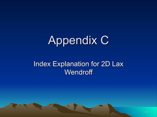
Download to read offline

![Introductions Bob Robey -- Los Alamos National Lab, X division [email_address] , 665-9052 or home: [email_address] , 662-2018 3D Hydrocodes and parallel numerical software Helped found UNM and Maui High Performance Computing Centers and Supercomputing Tutorials Randy Roberts -- Los Alamos National Lab, D Division Java, C++, Numerical and Agent Based Modeling [email_address] Cleve Moler Matlab Founder Former UNM CS Dept Chair SIAM President Author of “Numerical Computing with Matlab” and “Experiments with Matlab”](https://image.slidesharecdn.com/secretsofsupercomputing-110115094830-phpapp02/85/Secrets-of-supercomputing-2-320.jpg)
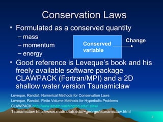

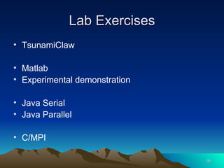
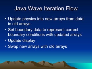
![Java Wave Structure Wave class does most of the work main(String[] args) calls start() start() creates a WaveProblemSetup start() calls methods to do initialization and boundary conditions start() calls methods to iterate and update the display](https://image.slidesharecdn.com/secretsofsupercomputing-110115094830-phpapp02/85/Secrets-of-supercomputing-29-320.jpg)
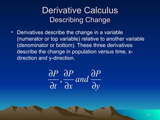
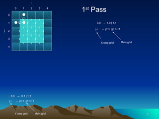
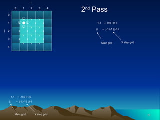

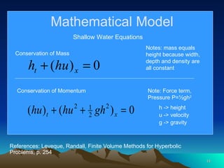
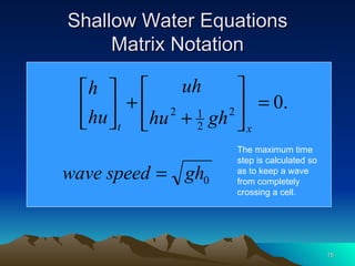
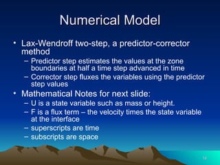
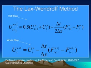
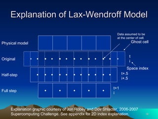
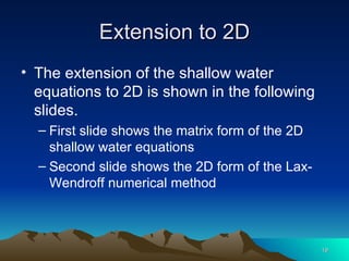
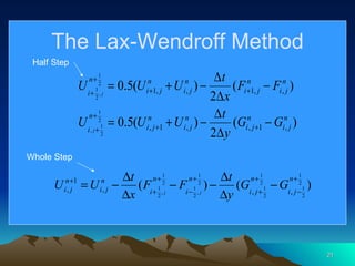
The document provides background on supercomputing and introduces the shallow water equations model for simulating wave motion. It describes: 1) The mathematical shallow water equations model for conserving mass and momentum over time. 2) The numerical Lax-Wendroff method used to solve the equations, including predictor-corrector steps. 3) Sample programs implementing the method in languages like C/MPI, Java, and MATLAB to model wave behavior in 1D and 2D.


![[Harvard CS264] 02 - Parallel Thinking, Architecture, Theory & Patterns](https://cdn.slidesharecdn.com/ss_thumbnails/cs264201102-archtheorypatternshare-110206154047-phpapp02-thumbnail.jpg?width=640&height=640&fit=bounds)


